Scaling relations for turbulence in the multiphase interstellar medium

Abstract

We employ a generalization of the She & Lévêque model to study velocity scaling relations based on our simulations of thermal instability–induced turbulence. Being a by-product of the interstellar phase transition, such multiphase turbulence tends to be more intermittent than compressible isothermal turbulence. Due to radiative cooling, which promotes nonlinear instabilities in supersonic flows, the Hausdorff dimension of the most singular dissipative structures, $D$, can be as high as 2.3, while in supersonic isothermal turbulence $D$ is limited by shock dissipation to $D\leqslant 2$. We also show that single-phase velocity statistics carry only incomplete information on the turbulent cascade in a multiphase medium. We briefly discuss the possible implications of these results on the hierarchical structure of molecular clouds and on star formation.

1 Introduction

Interstellar turbulence is believed to be neither incompressible nor isotropic nor homogeneous. Yet the observed velocity scaling relations in quite a variety of environments (Larson, 1979, 1981; Armstrong, Rickett, & Spangler, 1995) are surprisingly close to those predicted by Kolmogorov (1941a, hereafter K41). At the same time, turbulence in molecular clouds appears to be quite different in terms of velocity correlations, in some cases, with substantially super-Kolmogorov power indices for both first-order velocity structure functions and velocity power spectra (Brunt & Heyer, 2002). Interstellar turbulence is one of the key ingredients of modern theories of star formation. It appears to be the major shaping agent for the mass distribution of prestellar dense cores in star forming molecular clouds and, ultimately, it could determine the stellar initial mass function (Padoan & Nordlund, 2002). Therefore, it is important to understand what makes it so similar to incompressible Kolmogorov turbulence and when, where, and to what extent one should expect to see significant deviations of observed scaling relations from the predictions of K41 theory.

As is known, dissipation controls the scaling properties of turbulence through intermittency. Intermittency corrections to K41 theory for incompressible turbulence, in which the most singular dissipative structures are one-dimensional vortex filaments (She & Lévêque, 1994, hereafter SL94), differ from those for compressible supersonic turbulence, in which the structures are two-dimensional shock fronts (Boldyrev, 2002, hereafter B02). Direct numerical simulations of compressible isothermal turbulence support this heuristic theory, demonstrating that the dimension $D$ of the dissipative structures depends on the turbulent Mach number and changes from $D=1$ for subsonic to $D=2$ for highly supersonic flows (Padoan et al., 2003).

Obviously, the nature of dissipative processes in the interstellar medium (ISM) is distinct from that in most laboratory environments as well as in numerical simulations that assume ideal (magneto)hydrodynamics. What would the dissipative structures look like in the turbulent ISM where physical conditions are largely determined by competing cooling and heating processes? The shape of the net cooling function is known to be responsible for thermal instability (TI; Field 1965) that affects the ISM hydrodynamics in a number of ways, from creating multiple thermal phases coexisting at constant pressure (Pikel’ner, 1968; Field, Goldsmith, & Habing, 1969) to promoting nonlinear instabilities in cold shock-bounded slabs (Vishniac, 1994; Blondin & Marks, 1996). How effective are volumetric energy sources in shaping the velocity scalings in intermittent interstellar turbulence? We address this question here by means of three-dimensional numerical simulations of decaying hydrodynamic turbulence initiated by rapid thermally unstable radiative cooling. In this model, turbulence is a by-product of the phase transition in the hot gas that leads to the formation of a two-phase medium. This Letter is the third in our series on turbulence in the multiphase ISM (Kritsuk & Norman, 2002a, b). We refer the reader to our previous papers for the simulation details that are not covered here.

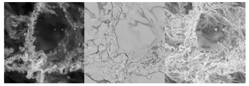
Figure 1: Snapshots of gas density ($\log{\rho}$, left panel), velocity divergence ($\nabla\cdot u$, middle), and vorticity magnitude [$\log(\nabla\times u)^{2}$, right], for a randomly chosen slice through the computational volume of $256^{3}$ zones at $t=0.12$ Myr. With a “standard” linear gray-scale color map, dense structures in the left panel are shown as scrambled bright filaments, accretion shocks in the middle as sharp dark rims framing the cross-section of the density “walls”, and vortex filaments in the right panel as delicate freshly cooked Capelli d’Angelo covering the overdense regions and extending into underdense voids where the Kolmogorov cascade has not quite fully developed yet.

2 Model description

We start the simulation with a periodic box of 5 pc on a side filled with hot ($2\times 10^{6}$ K) thermally unstable gas initially far from thermal equilibrium (only 2% of radiative cooling is compensated for by a constant uniform volumetric heating source). Small isobaric random Gaussian density perturbations (power spectrum index -3) are imposed to initiate TI while initial velocities are set to zero. We follow the formation of a turbulent two-phase medium by solving the equations of ideal gas dynamics (eqs. [6]-[9] in Field 1965), assuming zero conductivity, with the piecewise parabolic method of Colella & Woodward (1984) on a grid of $256^{3}$ zones. The equilibrium cooling function we use describes radiative energy losses for solar metallicity gas at temperatures $T\in[10,10^{8}]$ K.

With an initial gas density of 1 cm^-3, the timescales for cooling and TI are of the order of $0.1$ Myr. The evolution begins with the isobaric linear growth of the density perturbations for $\sim 0.05$ Myr followed by the formation of thermal pancakes — thin two-dimensional cool dense structures emerging on caustics of the velocity field (Sasorov, 1988). As the mean gas temperature drops and larger scale modes enter the nonlinear regime, a small-scale network of thermal pancakes that formed earlier in overdense regions collapses into larger scale accretion shock-bounded cold dense structures. At the end of this rapid cooling stage, the gas temperature $T\in[30,\;3\times 10^{5}]$ K and the flow becomes highly supersonic with mass-weighted rms Mach number $\langle M\rangle_{\rho}~{}\raise 1.29167pt\hbox{$>$}\kern-7.5pt{\lower 2.79857pt\hbox{$\sim$}}~{}15$. (A simulation initiated with a flat “white-noise” spectrum of density perturbations returned a substantially lower value of $\langle M\rangle_{\rho}~{}\raise 1.29167pt\hbox{$<$}\kern-7.5pt{\lower 2.79857pt\hbox{$\sim$}}~{}2$, highlighting the importance of large-scale modes of TI for generation of supersonic flows.) Barotropic instabilities, shocks, and nonlinear thin shell instabilities (Vishniac, 1994) coupled with TI effectively generate vorticity within the emerging cold dense phase. As a result, large-scale thermal pancakes (Meerson & Sasorov, 1987) arise turbulent. Figure 1 shows shock-bounded “walls” and underdense “voids” forming during the early turbulent relaxation period. The topology of dense structures in Figure 1 is far richer than that of two-dimensional shock fronts in supersonic ideal gas turbulence. This snapshot taken at $t=0.12$ Myr corresponds to the peak of the volume-weighted rms Mach number, $\langle M\rangle_{V}\approx 3$. When cooling is present in nonequilibrium supersonic flows like this, thin high-density shells get folded by instabilities into sheets of finite thickness with $D>2$.

As turbulent relaxation proceeds, gas settles to thermal equilibrium and thermal phases get separated with about $18$% of the volume filled with the cold phase and $\sim 40$% with the warm phase by $t=0.56$ Myr. As turbulence decays further, filling factors for both stable phases slightly grow at the expense of the intermediate thermally unstable regime. Since this two-phase medium is quasi-isobaric ($\Delta p/p\approx 6\ll\Delta\rho/\rho\approx 1000$) and since velocities inherited from the initial “violent relaxation” do not correlate with density, the Mach number depends on the gas density roughly as $M\propto\rho^{1/2}$ (see Fig. 2). This means that there are two different regimes of turbulence coexisting in such a two-phase medium: a subsonic regime with $M\sim 0.4$ in the space-filling warm phase and a supersonic one $M\sim 1.5$ in the cold phase. The Mach number–density relation is a distinct feature of turbulence in a two-phase medium. It is quite natural that velocity scaling relations in this case will not be identical to those for isothermal compressible turbulence. It is also clear that reconstruction of these relations based on observations of any single phase in a multiphase medium would not be an easy task. We will further illustrate these ideas in the following section by formally applying statistical analysis methods developed for turbulence research to our simulation data.

3 Velocity statistics

In order to follow the time evolution of the turbulent velocity field across different scales, we computed three-dimensional velocity power spectra for four snapshots taken at $t=0.12$, 0.56, 1.5, and 2.5 Myr (Fig. 2). We also decomposed the velocity field into a divergence-free solenoidal component $u_{s}$ ($\nabla\cdot u_{s}=0$, dotted lines) and a curl-free dilatational component $u_{d}$ ($\nabla\times u_{d}=0$, dashed lines), such that $u=u_{s}+u_{d}$. As turbulence develops and decays, the fractions of power contained in the solenoidal and dilatational components vary as a function of time and scale. At $t=0.12$ Myr, the power spectrum is dominated by dilatational modes on large scales. A “wave” of solenoidal modes generated by nonlinear instabilities propagates from small to large scales and overlaps with dilatational modes as turbulence develops. Earlier, at $t=0.07$ Myr, the dilatational spectrum follows a nearly perfect $k^{-2}$ law for the whole range of wavenumbers, characteristic of Burgers turbulence accompanying the formation of a multiscale network of thermal pancakes. At that moment, the contribution of solenoidal modes is negligibly small.

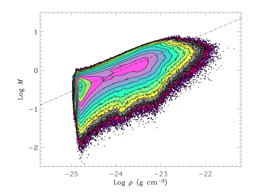
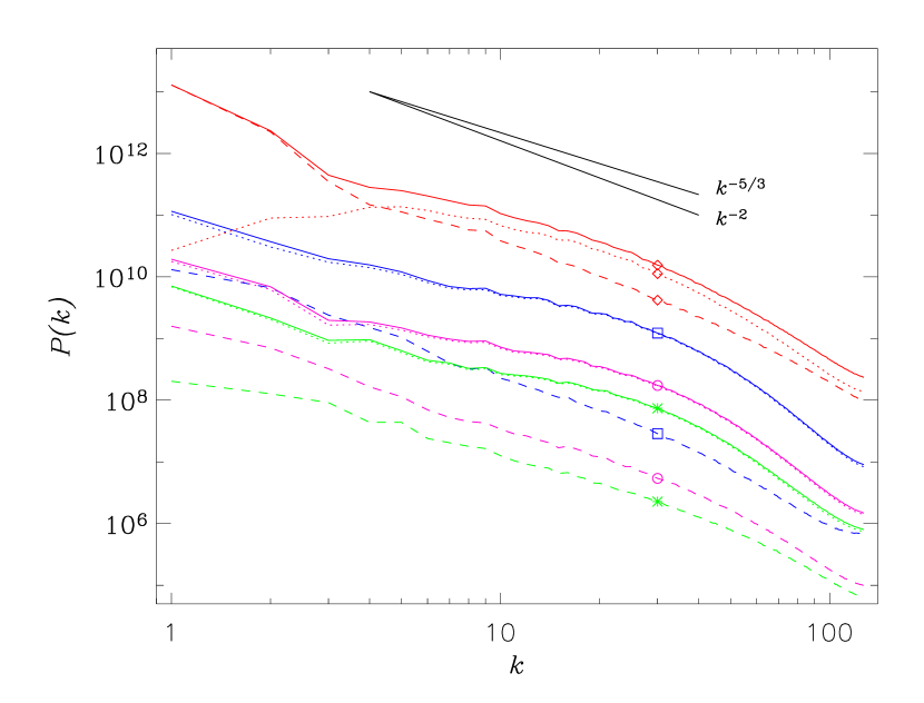
Figure 2: Left panel: Scatter plot of Mach number vs. gas density at $t=0.56$ Myr; contour levels are consecutive powers of 2, and the dash-dotted line follows the relation $M\propto\rho^{1/2}$ for isobaric gas with uncorrelated density and velocity. Right panel: Three-dimensional velocity power spectra (solid lines) for $t=0.12$ (diamond), 0.56 (square), 1.5 (circle), and 2.5 Myr (asterisk) decomposed into solenoidal (dotted lines) and dilatational (dashed lines) components. Also shown are the velocity power spectra for Kolmogorov (-5/3) and Burgers (-2) turbulence.

By $t=0.56$ Myr, solenoidal modes dominate on virtually all scales since dilatational modes decay much faster than solenoidal in an unforced regime that follows the initial phase transition. At $t=1.5$ Myr, the latter contribute only up to a few percent, making the dotted and solid lines in Figure 2 nearly indistinguishable. The dependence of power in solenoidal versus dilatational modes on the rms Mach number of the flow in our simulations is broadly consistent with the results of Boldyrev, Nordlund, & Padoan (2002b) for driven isothermal MHD turbulence.

To study scaling properties of the decaying turbulent cascade, we compute longitudinal and transverse velocity structure functions (SFs)

$$S_{p}(l)=\langle|u(x)-u(x+l)|^{p}\rangle\propto l^{\zeta_{p}}$$ (1)

(Monin & Yaglom, 1971) and exploit extended self-similarity (Benzi, et al., 1993, 1996) to obtain estimates for scaling exponents $\zeta_{p}$ relative to the third-order exponent: $S_{p}\propto S_{3}^{\zeta_{p}/\zeta_{3}}$. These relative scaling exponents may be more universal than $\zeta_{p}$ themselves since it is natural to use a generalized scale $\ell(l,\eta)$ instead of the resolution scale $l$ for the investigation of the scaling properties of turbulence (Dubrulle, 1994). A value of $\zeta_{3}$ is still required to recover the absolute values of the exponents $\zeta_{p}$, e.g., to get an estimate for the velocity power spectrum scaling in the inertial range $P(k)\propto k^{-1-\zeta_{2}}$. A rigorous result $\zeta_{3}=1$ holds for incompressible Navier-Stokes turbulence (Kolmogorov (1941b) “$4/5$” law) and for incompressible MHD (Politano, & Pouquet, 1998). Numerical simulations support the same result for supersonic compressible hydrodynamics (Porter, Pouquet, & Woodward, 2002, hereafter PPW02), but it is unclear whether this remains true in the presence of a generic volumetric energy source.

A three-parameter model developed by She & Lévêque (1994) and generalized by Dubrulle (1994) represents the turbulent energy cascade as an infinitely divisible log-Poisson process and relates the dimensionality of the most dissipative structures $D$ to the relative scaling exponents:

$$\frac{\zeta_{p}}{\zeta_{3}}=(1-\Delta)\Theta p+\frac{\Delta}{1-\beta}(1-\beta^{\Theta p}),$$ (2)

where $\beta\equiv 1-\Delta/(3-D)$ measures the “degree of nonintermittency” of energy dissipation, $\beta\in(0,1)$. The other two parameters represent nonintermittent scalings for the velocity difference, $u_{l}\propto l^{\Theta}$, and for the eddy turnover time scale, $t_{l}\propto l^{\Delta}$. For the Kolmogorov cascade, $\Theta=\frac{1}{3}$ and $\Delta=\frac{2}{3}$. In the limit $\beta\to 1$, the system is nonintermittent, and the K41 relation can readily be recovered. Since $\beta\to 0$ as $D\to 2\frac{1}{3}$, the model is only consistent with $D<2\frac{1}{3}$. Vortex filaments in incompressible turbulence are characterized by $D=1$ with which eq. (2) reduces to SL94 formula. In a series of numerical experiments on isothermal compressible turbulence with Mach numbers $0.62\leqslant M\leqslant 10$, Padoan et al. (2003) were able to trace a smooth transition from scalings that can be approximated by equation (2) with $D=1$ to those with $D=2$. Their result is consistent with the suggestion that velocity SF scaling for compressible turbulence can be described by the She-Lévêque formalism for any value of the Mach number of the flow, with only one parameter, $D$, varying as a function of $M$.

What kind of scaling can we expect for our model with a “realistic” nonisothermal scale-dependent effective equation of state determined by cooling and heating? How will it evolve as turbulence decays and the two phases settle into thermal and pressure equilibrium?

We computed velocity SFs up to the sixth order using the so-called XYZ method (see, e.g., PPW02). Relative scaling exponents for the same four snapshots that we used for power spectra are shown in Figure 3. We consider the difference between exponents for longitudinal and transverse SFs as a good quality indicator for the derived scalings (larger symbols show larger statistical uncertainties). We attribute this difference to poor statistics and to small deviations from full isotropy in our numerical model due to an insufficiently large value of the Reynolds number and the slightly anisotropic initial forcing on scales approaching the box size.

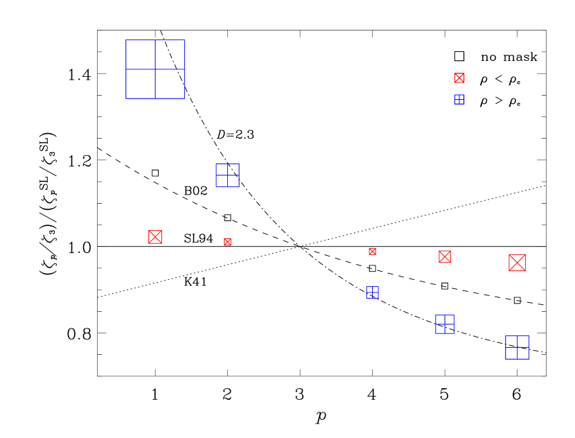
Figure 3: Scaling exponents for velocity structure functions of the orders 1–6 normalized by the SL94 model (horizontal solid line); other models include K41 (dotted line), B02 (dashed line), and eq. (2) with a fractal dimension $D=2.3$ (dash-dotted line). Symbol sizes show the difference between the longitudinal and transverse structure functions with a floor value. Left panel: Four snapshots illustrating the evolution of the scaling. The insert shows the kinetic energy as a function of time and timing for the snapshots: 0.12 (diamonds), 0.56 (squares), 1.5 (circles), and 2.5 Myr (asterisks). The legend in the upper right-hand corner gives volume- and mass-weighted rms Mach numbers for the snapshots. Right panel: Scaling exponents for a snapshot at $t=0.56$ Myr. The open squares are the same as in the left panel; the crossed squares show the exponents obtained with density masks $\rho\gtrless\rho_{c}=10^{-24.3}$ g cm^-3 and probe velocity correlations in the cold and warm phases separately.

Our results generally agree with those of Padoan et al. (2003) in the sense that the exponents in Figure 3 can be well described by equation (2) and, as the turbulence decays and becomes less supersonic, $D\to 1$. However, for a given turbulent Mach number, the value of $D$ appears to be larger in our multiphase case than in the isothermal turbulence. This could potentially be caused by the possibility that $\zeta_{3}<1$ in our case; higher resolution simulations would help to test this option. It is tempting to note that our first snapshot (diamonds), which corresponds to the most supersonic regime with no clear distinction between the thermal phases, demonstrated the maximal value of $D$ for this run which is approaching the upper bound of $2\frac{1}{3}$ from below. Curiously enough, this value coincides with the observationally determined fractal dimension of molecular clouds $D=2.3\pm 0.3$ (Elmegreen & Falgarone, 1996). We refer to Boldyrev et al. (2002b) for a relation between density and velocity correlators. It seems, however, that it is not the limited numerical resolution, but rather the lack of cooling-related instabilities that prevents dense structures from folding into a fractal distribution with dimensionality $D~{}\raise 1.29167pt\hbox{$>$}\kern-7.5pt{\lower 2.79857pt\hbox{$\sim$}}~{}2$ in simulations of isothermal turbulence (cf. Boldyrev, Nordlund, & Padoan 2002a). We will address the effects of magnetic fields and gas self-gravity on the dimension of the dissipative structures in a subsequent paper.

Observational diagnostics of turbulent velocity fluctuations in the ISM are usually based on phase-specific spectral line transitions. Since we model the formation of a turbulent two-phase medium, it is natural to compute SFs by measuring the velocity differences within a single phase and then to compare the results for both phases. We introduced two masks based on a gas density value of $\rho_{c}=10^{-24.3}$ g cm^-3 and obtained velocity SFs separately for zones where the gas density is higher or lower than the threshold $\rho_{c}$, which is close to the lower bound of a thermally unstable regime (for gas in thermal equilibrium) and, thus, separates the warm stable phase from cold “clouds” and unstable gas. At $t=0.56$ Myr, the filling factors for both density regimes are about 50%.

The scaling exponents for velocity SFs of low- and high-density gas are shown in Figure 3. The statistics for both density regimes are relatively poor as is indicated by the size of the crossed symbols. They are good enough, however, to conclude that the cold-phase exponents show significantly larger departures from K41 scalings than do the complete statistics unaffected by masking. The crossed symbols representing the warm phase instead demonstrate more K41-like scalings. Both transverse and longitudinal SFs follow the trend outlined above, but the exponents for transverse SFs show consistently smaller departures from the unbiased exponents. We conclude that the velocity power spectrum index $n_{c}$ based on observations of the cold molecular phase would instead be an upper estimate for the actual index $n=1+\zeta_{2}$, while $n_{w}$ determined from the warm gas velocities would only give a lower bound for $n$.

4 Conclusions

We considered a simple model for TI-induced decaying hydrodynamic turbulence in a radiatively cooling medium with a low constant heating rate. A formal application of the She & Lévêque (1994) model to the simulated velocity fields consistently showed that cooling-related instabilities make turbulence in multiphase gas more intermittent than conventional compressible supersonic turbulence. This result could have interesting implications for the recently developed turbulent fragmentation branch of star formation theory. Finally, we demonstrated that phase-specific observational velocity statistics for multiphase media can be affected by the correlation of a turbulent Mach number with gas density.

References

- Armstrong, Rickett, & Spangler (1995) Armstrong, J. W., Rickett, B. J., & Spangler, S. R. 1995, ApJ, 443, 209
- Benzi, et al. (1993) Benzi, R., Ciliberto, S., Tripiccione, R., Baudet, C., Massaioli, F., Succi, S. 1993, Phys. Rev. E, 48, R29
- Benzi, et al. (1996) Benzi, R., Biferale, L., Ciliberto, S., Struglia, M.V., Tripiccione, R. 1996, Physica D, 96, 162
- Blondin & Marks (1996) Blondin, J. M. & Marks, B. S. 1996, New Astronomy, 1, 235
- Boldyrev (2002) Boldyrev, S. 2002, ApJ, 569, 841 (B02)
- Boldyrev, Nordlund, & Padoan (2002a) Boldyrev, S., Nordlund, Å., & Padoan, P. 2002a, ApJ, 573, 678
- Boldyrev, Nordlund, & Padoan (2002b) Boldyrev, S., Nordlund, Å., & Padoan, P. 2002b, Phys. Rev. Lett., 89, 31102
- Brunt & Heyer (2002) Brunt, C. M. & Heyer, M. H. 2002, ApJ, 566, 289
- Colella & Woodward (1984) Colella, P. & Woodward, P. R. 1984, J. Comp. Phys., 54, 174
- Dubrulle (1994) Dubrulle, B. 1994, Phys. Rev. Lett., 73, 959
- Elmegreen & Falgarone (1996) Elmegreen, B. G. & Falgarone, E. 1996, ApJ, 471, 816
- Field (1965) Field, G. B. 1965, ApJ, 142, 531
- Field, Goldsmith, & Habing (1969) Field, G. B., Goldsmith, D. W., & Habing, H. J. 1969, ApJ, 155, L149
- Kolmogorov (1941a) Kolmogorov, A. N. 1941a, Dokl. Akad. Nauk SSSR, 30, 299 (K41)
- Kolmogorov (1941b) Kolmogorov, A. N. 1941b, Dokl. Akad. Nauk SSSR, 32, 19
- Kritsuk & Norman (2002a) Kritsuk, A. G., & Norman, M. L. 2002a, ApJ, 569, L127
- Kritsuk & Norman (2002b) Kritsuk, A. G., & Norman, M. L. 2002b, ApJ, 580, L51
- Larson (1979) Larson, R. B. 1979, MNRAS, 186, 479
- Larson (1981) Larson, R. B. 1981, MNRAS, 194, 809
- Meerson & Sasorov (1987) Meerson, V. I., & Sasorov, P.V. 1987, Soviet Phys.–JETP, 65, 300
- Monin & Yaglom (1971) Monin, A. S., & Yaglom, A. M. 1971-75, Statistical Fluid Mechanics; Mechanics of Turbulence, Vols. 1 and 2, (Cambridge, MA: MIT Press)
- Padoan et al. (2003) Padoan, P., Jimenez, R., Nordlund, A., & Boldyrev, S. 2003, astro-ph/0301026
- Padoan & Nordlund (2002) Padoan, P. & Nordlund, Å. 2002, ApJ, 576, 870
- Pikel’ner (1968) Pikel’ner, S. B. 1968, Soviet Astron., 11, 737
- Politano, & Pouquet (1998) Politano, H., Pouquet, A. 1998, Geophys. Res. Lett., 25, 273
- Porter, Pouquet, & Woodward (2002) Porter, D., Pouquet, A., & Woodward, P. 2002, Phys. Rev. E, 66, 026301 (PPW02)
- Sasorov (1988) Sasorov, P. V. 1988, Soviet Astron. Lett., 14, 129
- She & Lévêque (1994) She, Z.-S., & Lévêque, E. 1994, Phys. Rev. Lett., 72, 336 (SL94)
- Vishniac (1994) Vishniac, E. T. 1994, ApJ, 428, 186