A high-resolution study of nonthermal radio and X-ray emission from SNR G347.3–0.5

Abstract

G347.3–0.5 is one of three shell-type supernova remnants in the Galaxy whose X-ray spectrum is dominated by nonthermal emission. This puts G347.3–0.5 in the small, but growing class of SNRs for which the X-ray emission reveals directly the presence of extremely energetic electrons accelerated by the SNR shock. We have obtained new high-resolution X-ray and radio data on G347.3–0.5 using the Chandra X-ray Observatory and the Australia Telescope Compact Array (ATCA) respectively. The bright northwestern peak of the SNR seen in ROSAT and ASCA images is resolved with Chandra into bright filaments and fainter diffuse emission. These features show good correspondence with the radio morphological structure, providing strong evidence that the same population of electrons is responsible for the synchrotron emission in both bands in this part of the remnant. Spectral index information from both observations is presented. We found significant difference in photon index value between bright and faint regions of the SNR shell. Spectral properties of these regions support the notion that efficient particle acceleration is occurring in the bright SNR filaments. We report the detection of linear radio polarization towards the SNR, which is most ordered at the northwestern shell where particle acceleration is presumably occurring. Using our new Chandra and ATCA data we model the broad-band emission from G347.3–0.5 with the synchrotron and inverse Compton mechanisms and discuss the conditions under which this is a plausible scenario.

1 INTRODUCTION

Due to the release of an enormous amount of energy ($\sim 10^{51}$ erg) at their creation, supernova remnants (SNRs) have long been considered as a primary source of Galactic cosmic rays with energies up to the “knee” of the spectrum at $\sim 3\times 10^{15}$ eV (Shklovsky, 1953; Ginzburg, 1957). Cosmic rays with energies higher than this are believed to be extragalactic in origin (Axford, 1994). First-order Fermi shock acceleration, also called diffusive shock acceleration, in which particles gain energy from scattering back and forth across the shock, has been suggested as the most probable acceleration mechanism in SNR shocks (see Reynolds & Chevalier, 1981; Blandford & Eichler, 1987; Jones & Ellison, 1991). However, until recently the observational evidence for the production of high energy particles in SNRs was poor and came mainly from the fact that SNRs emit synchrotron radiation in the radio band. The major observational break-through came only recently with the detection of nonthermal X-ray emission from the shell-type SNR SN 1006 (Koyama et al., 1995). The featureless X-ray spectrum found at the rim of SN 1006, in contrast to the thermal spectra found towards the interior of the remnant, was fitted well with a power law of photon index $\Gamma\sim 2.2$ (where the photon flux $F$ obeys $F\propto(h\nu)^{-\Gamma}$). Further evidence came with the detection of TeV $\gamma$-ray emission from SN 1006 (Tanimori et al., 1998). There are several mechanisms capable of producing TeV energy photons, including inverse Compton (IC) scattering, nonthermal bremsstrahlung and pion-decay. Broad-band modeling of the emission from SN 1006 indicates that IC scattering is responsible for the TeV $\gamma$-ray emission (e.g., Mastichiadis & de Jager, 1996; Allen, Petre, & Gotthelf, 2001). However, cosmic rays are comprised mostly of protons and there is not yet clear evidence of proton acceleration in SNRs, aside from the suggestion that the TeV emission results from neutral pion-decay (Aharonian & Atoyan, 1999; Enomoto et al., 2002). Another problem in the quest for a cosmic ray origin in SNRs is that the maximum energy of electrons produced by SNRs seems to fall below the “knee”. For example, studies of about 20 SNRs with mostly thermal X-ray emission imply that the maximum energy to which electrons can be accelerated does not exceed $10^{14}$ eV (Reynolds & Keohane, 1999; Hendrick & Reynolds, 2001).

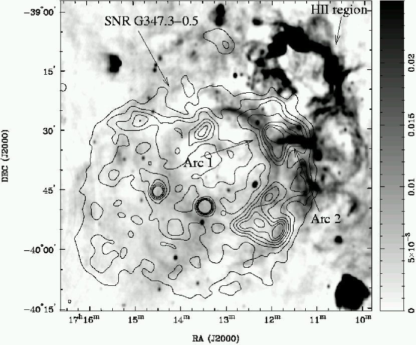
Figure 5: ATCA images of G347.3–0.5 and surrounding region at 1.4 GHz. The image was convolved with a Gaussian restoring beam of $46\arcsec\times 36\arcsec$ (P.A.= $-$3.8), shown by the tiny ellipse in the bottom left corner. The image is overlaid with the ROSAT contours with the levels same as in Figure 1. The linear grayscale is in units Jy beam^-1.

Two more shell-type remnants with dominant non-thermal X-ray spectra have been identified: G347.3–0.5 (Koyama et al., 1997; Slane et al., 1999) and G266.2–1.2 (Slane et al., 2001). G347.3–0.5 (RX J1713.7–3946) was first discovered in the ROSAT (Röntgensatellit) All-Sky Survey by Pfeffermann & Aschenbach (1996), who used a thermal plasma model to infer a very high temperature of $kT\sim 4.8$ keV, and column density of $N_{H}\sim 4.5\times 10^{21}$  cm^-2. Based on this column density the distance to the SNR was estimated to be $\sim 1.1$ kpc, while the derived plasma temperature implied an SNR age of $\sim 2100$ yrs. However, subsequent ASCA (Advanced Satellite for Cosmology and Astrophysics) observations revealed that the X-ray emission from the remnant is predominantly nonthermal (Koyama et al., 1997; Slane et al., 1999). The remnant is $\sim 1$° in diameter and appears to be of a shell–type morphology with the brightest emission in the western region. The SNR is located on the edge of the molecular cloud complex that encompasses the H ii region G347.61+0.20 located northwest of the SNR (see Figure 5). Assuming that the SNR is physically associated with the molecular cloud complex, the distance was estimated to be $6.3\pm 0.4$ kpc from existing observations of the CO 1–0 line emission towards the complex (Slane et al., 1999). ASCA observations did not reveal any line emission from the SNR interior, and this lack of thermal emission sets an upper limit on the mean density around the remnant of $<0.3$  cm^-3 (Slane et al., 1999). Such a low density suggests that the majority of the remnant is still evolving in the interior of the large circumstellar cavity driven by the wind of its massive progenitor. In the northwestern region of G347.3–0.5, where the SNR may be interacting with denser molecular gas, the upper limit on the ambient density is higher ($<1$  cm^-3), which is broadly consistent with the densities estimated around other SNRs that are associated with molecular clouds. Most recently, Pannuti et al. (2003) reported detection of a thermal component towards the center of the SNR, which implies gas density of 0.05–0.07 cm^-3 in this part of the SNR.

Two point sources have been identified within the boundaries of the remnant shell: 1WGA J1714.4–3945 is believed to be of stellar origin (Pfeffermann & Aschenbach, 1996), while 1WGA J1713.4–3949 is located at the center of the SNR, has no obvious optical counterpart, and is a candidate for an associated neutron star (Slane et al., 1999). Our Chandra observations also included the latter point source, results for which are presented elsewhere (Lazendic et al., 2003).

G347.3–0.5 was also detected at TeV energies with the CANGAROO telescope (Muraishi et al., 2000; Enomoto et al., 2002), and models of broad-band emission point to IC scattering as the origin of the TeV photons (Muraishi et al., 2000; Ellison, Slane, & Gaensler, 2001). More recently, follow up TeV $\gamma$-ray observations have led to a different conclusion, suggesting pion-decay as the source of energetic photons (Enomoto et al., 2002), but the nature of this emission is still uncertain (see Butt et al., 2002; Reimer & Pohl, 2002). An EGRET source 3EG J1714–3857 (Hartman et al., 1999) was also detected near the remnant and linked to the SNR interaction with a molecular cloud (Butt et al., 2001). This is potentially supported by the identification of the hard X-ray source AX J1714.1–3912, which appears to coincide with the location of one of the molecular clouds in the complex, and possibly with the EGRET source (Uchiyama, Takahashi, & Aharonian, 2002). However, the energetics required to yield the observed X-ray flux of the source appear problematic relative to the total energy budget of the SNR unless the source distance is a factor of five smaller than suggested by the molecular line velocity of the cloud.

To investigate the fine-scale structure of the SNR and its relationship with particle acceleration, we obtained high-resolution X-ray and radio data on G347.3–0.5 using the Chandra X-ray Observatory and the Australia Telescope Compact Array (ATCA). Our goal was to look for spectral variations in different spatial regions, to improve the estimates on thermal emission, to compare the X-ray morphology with high-resolution radio images, to correlate the radio and X-ray spectral indices and to investigate linear polararization. We present these results here, along with modeling of the broad-band spectrum of G347.3–0.5 to investigate the origin of the accelerated high energy particles in this SNR.

In section $\S$ 2 we describe our X-ray observations, and present images and spectral results for the SNR. Radio observations and images of the SNR are presented in section $\S$3, where we also derive a radio spectral index and measure linear polarization in the SNR. In section $\S$4 we discuss the spectral variations across the nortwestern SNR shell and in section $\S$5 we investigate the SNR morphology and the correlation between X-ray and radio images. In section $\S 6$ we present synchrotron and inverse Compton modeling of the broad-band spectrum from G347.3–0.5 and discuss the origin of the TeV emission in this SNR.

2 X-RAY DATA

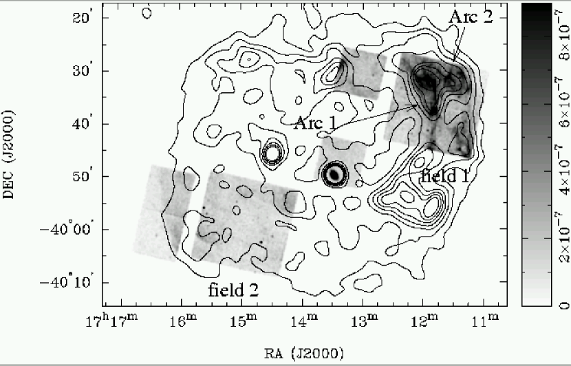
Figure 1: The 1.0–8.0 keV band Chandra ACIS greyscale image of G347.3–0.5, including the central source 1WGA J1713.4–3949 which appears elongated due to off-axis location in the ACIS-S1 chip (see Lazendic et al., 2003, for details on this source). The linear greyscale is in units counts arcsec^-2 s^-1 and is saturated to show regions with low emission. To show the whole extent of the remnant, the Chandra image is overlaid with the ROSAT PSPC contours (Slane et al., 1999). Contour levels are: 7, 12, 17, 22, 27, 32, 37 $\times$ 0.018 counts arcmin^-2 s^-1. Two bright arcs, observed in radio band (see Figure 5), are labeled: Arc 1, of which Chandra covered southwestern portion, extends approximately north-south, while Arc 2 is almost perpendicular to Arc 1. The two observed Chandra fields are also labeled as field 1 and field 2.

G347.3–0.5 was observed with the Advanced CCD Imaging Spectrometer (ACIS) detector on board the Chandra X-ray Observatory on 2000 July 25. ACIS consists of two CCD arrays — the ACIS-I (Imaging) array has four CCDs arranged in a square, while the ACIS-S (Spectroscopic) array has six linearly adjacent CCDs. Only six CCDs can be used at one time. The angular size of G347.3–0.5 is much larger than the ACIS-I field of view ($16\farcm 9\times 16\farcm 9$), so we observed two diametrically opposed fields covering regions of the SNR shell, as shown in Figure 1. Field 1 (ObsId 736) was centered on the bright northwestern rim at ${\rm RA}={17}^{\rm h}{11}^{\rm m}{49}\fs{8}$, ${\rm Dec.}={-39}^{\circ}{36}\arcmin{18}\farcs{0}$ and consisted of a 30 ks exposure. Field 2 (ObsId 737) was observed for 40 ks, positioned at the fainter eastern SNR rim centered at ${\rm RA}={17}^{\rm h}{15}^{\rm m}{16}\fs{5}$, ${\rm Dec.}={-39}^{\circ}{57}\arcmin{56}\farcs{0}$. Two ACIS-S chips were also turned on: for field 1, the ACIS-S1 and ACIS-S3 chips were used to include the central point source and a region in the SNR interior, while for field 2 ACIS-S2 and ACIS-S3 were used to cover the eastern SNR rim. Data were taken in full-frame timed–exposure (TE) mode with the standard integration time of 3.2 s.

Data were reduced using standard threads in the Chandra Interactive Analysis of Observations (CIAO) software package version 2.2.1. To mitigate the degradation in the spectral response of the ACIS chips caused by radiation damage early in the mission (see Prigozhin et al., 2000), we also used software (Townsley et al., 2000, 2002) to correct for the effect of increased charge transfer inefficiency (CTI), such as gain variations, event grade distortion and degraded energy resolution as a function of row number in each CCD. These corrections increase the number of detected events and improve the assigned event energies and spectral resolution. We applied CTI corrections to the Level 1 processed event list provided by the pipeline processing done at the Chandra X-ray Center (CXC). The data were then screened for “flaring” pixels and filtered with standard ASCA grades (02346). The effective exposure time after data processing was 29.6 ks and 38.9 ks for field 1 and 2, respectively.

2.1 X-ray Image

We used the CIAO script merge_all to combine the data from the two fields into an exposure-corrected X-ray image in the energy range 1–8 keV. Since the effective area of the detector depends both on the energy of incident photons and their positions on the CCD, we applied spectral weighting to the merged image, which takes into account the fraction of the incident flux falling in the particular part of the band. The exposure-corrected image was blanked where the exposure was less than 15% of its maximum value. The final image is shown in Figure 1 overlaid with the ROSAT contours. The image was binned in $4\farcs 6\times 4\farcs 6$ pixels and smoothed with a Gaussian filter with a FWHM of 2″. Since CTI corrections were not available for ACIS-S1 chip on which the central source is located, these data were processed separately and then added to the image. We also made soft (0.5–2.1 keV) and hard band (2.1–8.0 keV) images, but they do not show any significant brightness variation with energy.

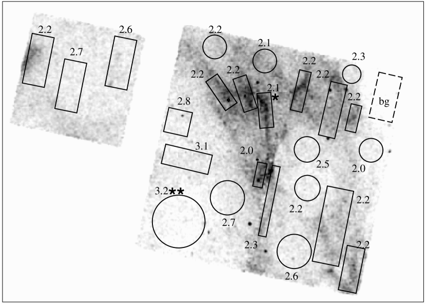
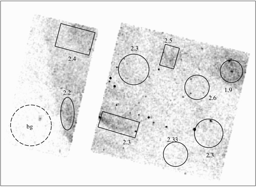
Figure 2: Extraction regions from field 1 and 2 and their corresponding best-fit photon index values. The regions outlined with the dashed line are used for background subtraction.

The northwestern peak seen in ROSAT and ASCA images is resolved with Chandra observations into two bright arcs and fainter diffuse emission, as shown in Figure 1. As we discuss below, this structure bears significant resemblances to what is seen in radio images. Arc 1 (see Figure 1 and Figure 2) appears to be made of thin filaments delineating the SNR shock front, while Arc 2 has a more irregular shape. Diffuse emission along the eastern shell does not show significantly different structure from that seen with ROSAT, although the limb is more clearly defined and extends beyond contours obtained from the ROSAT image.

2.2 X-ray Spectra

X-ray spectra were extracted from discrete regions of the ACIS chips in field 1 and field 2, shown in Figure 2. For each spectrum the counts were grouped with a minimum of 25 counts per spectral channel. We use redistribution matrix files (RMF) appropriate for CTI-corrected data (Townsley et al., 2000, 2002), and created weighted auxiliary response files (ARF) applying the same spectral binning as used in the corresponding RMFs. The background for the spectral fitting was extracted from the northwest corner in field 1 and from the southeast corner in field 2 (see Figure 2).

Shock acceleration of electrons to X-ray emitting energies is expected to produce a roughly power law distribution with an exponential cutoff above some maximum energy, resulting in a photon spectrum rolling slowly off through the X-ray band. The Chandra bandpass is not large enough in most cases to distinguish this slight curvature from a strait power law. The X-ray slope bears no particular relation to the slope at lower frequencies, but can serve as an indication of the location of the rolloff. We shall use both power law fits (giving photon index $\Gamma$) and cutoff-model fits (SRCUT, giving a rolloff frequency) to describe our spectra.

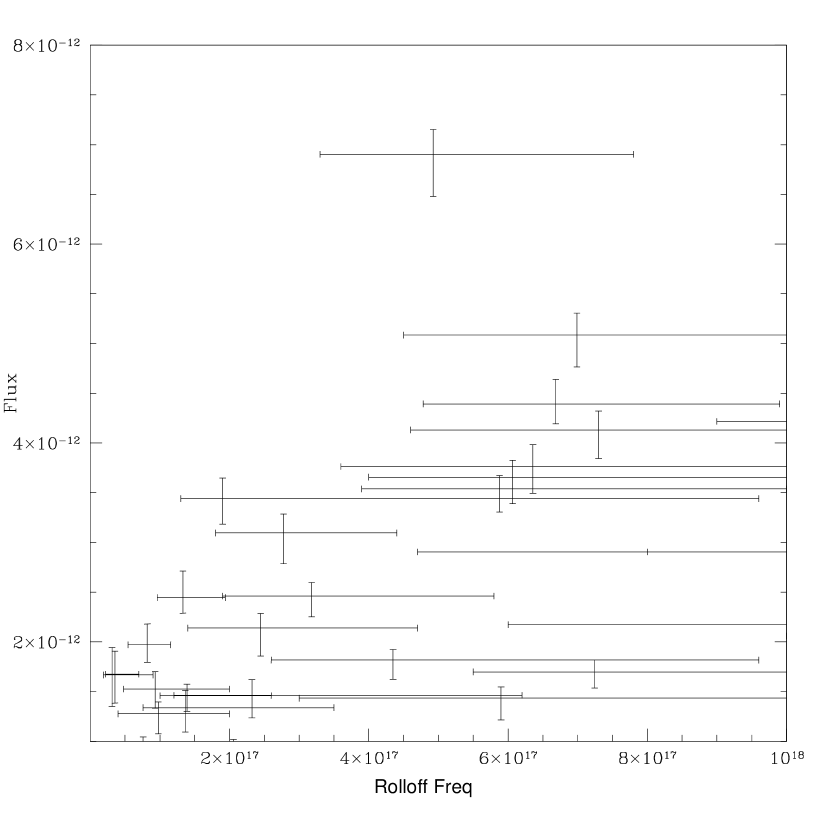
Figure 3: The best-fit values of X-ray flux and photon index/rolloff frequency values with 90% confidence level derived from power law and SRCUT model fits to the spectra from regions in field 1 and field 2 marked in Figure 2.

Individual spectra were first fitted separately to search for any change in the photon index across the source and for the presence of thermal component. We found small-scale spectral differences in different regions. We could fit those either with variations in column density, and roughly the same photon index ($\sim 2.1$), or, if the column density were fixed, with variations in the photon index. In the first case, we found that the column density was higher towards the bright regions ($\sim 8\times 10^{21}$ cm^-2) than towards the fainter regions ($\sim 5\times 10^{21}$ cm^-2). Thus, the brighter regions have higher column density, which is opposite from what one expects if the brightness variation is caused by varying interstellar absorption. Furthermore, the fact that the radio and X-ray emission have the similar morphologies in field 1 implies that X-ray brightness distribution is not the result of variations in absorption. Thus, it seems plausible that the column density is constant across field 1 and we adopt the second case, fixing the column density at the value found in the spatially averaged fitting and allowing $\Gamma$ to vary. Photon index values derived with the second approach are plotted in Figure 3 and imply that there is significant spectral variation between the bright and the faint SNR regions. The bright emission has values $2.05<\Gamma<2.25$, while the faint emission takes broad range of values, with the steepest photon index of $\sim 3$. Representative spectra with power law model fit are shown in Figure 4. The average values of photon index across field 1 of $\sim 2.35$ is consistent with that of $2.41$ for the northwestern region from the previous study with ASCA (Slane et al., 1999).

We then fitted our data with the SRCUT model (Reynolds & Keohane, 1999), which calculates a synchrotron spectrum from a power law distribution of electrons modified by an exponentially cut off in a uniform magnetic field. The model can be used to derive the maximum rolloff frequency $\nu_{rolloff}$ related to the maximum electron energy. Derived $\nu_{rolloff}$ values are plotted in Figure 3. We frozen the radio spectral index $\alpha$ (where the radio flux $S_{\nu}\propto\nu^{-\alpha}$) parameter for each spectrum to the global SNR value of 0.6 and left normalization (i.e., the 1 GHz radio flux density) as a free parameter. The model gave reduced $\chi^{2}$ value comparable to that of the power law model and the range of values for rolloff frequency between 3$\times 10^{16}$–2$\times 10^{18}$ Hz, with the fainter regions having, in generall, lower $\nu_{rolloff}$ values.

The SNR spectra from regions we observed with Chandra show no evidence for any emission lines. Adding equilibrium or non-equilibrium thermal models to the power law fits of the individual or joint fit to the spectra does not improve the fit significantly. However, spectra from some regions in both ACIS-S3 chips show a possible line feature around 0.8 keV. Modeling this feature does not provide strong constraints on the thermal emission properties, so deeper observations are needed to follow up this potential detection of thermal emission in G347.3–0.5.

3 RADIO DATA

Radio observations of G347.3–0.5 were obtained with the ATCA during January, March and April 1998. The array consists of six 22 m antennas that can be configured to give baselines between 31 m and 6 km (see Frater, Brooks, & Whiteoak, 1992). We used the array in three different configurations (375, 750 A and 1.5 A) to provide optimal $uv$-coverage of the observed region. Due to the large extent of the SNR and the complexity of the field around it, the region was imaged in mosaic mode with 10 pointing centers. Data were taken simultaneously at two frequencies, 1.4 and 2.5 GHz, each using a bandwidth of 128 MHz split in 32 4-MHz channels. For all the observations the primary calibrator PKS B1934–638 was used for bandpass and absolute flux calibration. PKS 1740–517 was used as a secondary calibrator for antenna gains and instrumental polarization calibration.

3.1 Radio Images

Radio data were reduced using standard procedures of the MIRIAD software package (Sault & Killeen, 2001). In the editing procedure, 4 channels on each side of the band were discarded and the remaining 26 central channels were averaged down to 13 8–MHz channels by Hanning smoothing. A uniform weighting was applied to visibilities to minimize sidelobes in the images. The longest baselines (i.e., all correlations with the sixth antenna) were excluded to enhance the surface brightness sensitivity. Also, amplitude and phase self-calibration were applied to the 1.4 GHz data to improve solutions for antenna gains using a strong point source in the eastern edge of the observed field (outside the image shown here). The images were made using the multi-frequency synthesis (Sault & Wieringa, 1994) and deconvolved using the mosaiced maximum entropy approach (Sault, Staveley-Smith & Brouw, 1996). The resulting images were convolved with a Gaussian restoring beam listed in Table 1, and corrected for primary beam response. The rms sensitivity in the images is also listed in Table 1.

In Figure 5 we show the image at 1.4 GHz overlaid with the ROSAT contours. As noted by Slane et al. (1999), in the radio band the SNR appears as a faint shell with two bright arcs to the west (marked in Figure 5). A faint inner ring of emission is also evident in the radio image of the SNR (Figure 5), with a diameter of $\sim 30\arcmin$. The image at 1.4 GHz has angular resolution comparable to the Molonglo Observatory Synthesis Telescope (MOST) image (Slane et al., 1999) and was published in preliminary form by Ellison, Slane, & Gaensler (2001). While the image at 2.5 GHz has improved angular resolution, it shows no significant morphological difference with respect to the other two images, and thus we do not show it here.

We find no obvious radio source at the location of the ASCA source AX J1714.1–3912, believed to be associated with the EGRET source 3EG J1714–3857 in the vicinity of the SNR (Uchiyama, Takahashi, & Aharonian, 2002). There are, however, a few compact radio sources around that location which are probably thermal H ii regions.

3.2 Radio Spectral Index

To determine the spectral index of the bright western SNR rim, we used the “spectral tomography” approach (Katz-Stone & Rudnick, 1997). Since source visibilities at different frequencies are sampled with different $u-v$ spacings, we first had to resample the 1.4 GHz data to match the $uv$-coverage of the 2.5 GHz data (see e.g., Crawford et al., 2001). We first removed the primary beam attenuation from the 1.4 GHz image, to which we then applied the primary beam attenuation and mosaic pattern of the 2.5 GHz data. The resulting image was Fourier transformed and resampled using the transfer function of the 2.5 GHz data. We then imaged and deconvolved these modified 1.4 GHz data using the same procedures as for the 2.5 GHz data. The modified 1.4 GHz and original 2.5 GHz image were then both smoothed to a resolution of 60″. The 2.5 GHz image was scaled by a trial spectral index, $\alpha_{t}$, and subtracted from the 1.4 GHz image, $I_{\alpha_{t}}=I_{1.4}-(1.4/2.5)^{\alpha_{t}}I_{2.5}$, where $I_{\alpha_{t}}$ is the difference image, and $I_{1.4}$ and $I_{2.5}$ are the images at 1.4 and 2.5 GHz, respectively. The spectral index $\alpha$ is then found as the value of $\alpha_{t}$ at which a particular feature in the image blends into the background, while the range of $\alpha_{t}$ values for which the residuals of the blended feature are significant gives the uncertainty in the spectral index.

We find a spectral index of $0.50\pm 0.40$ for the bright northwestern region of the SNR. This large uncertainty in the spectral index determination is caused by calibration errors and dynamic range limitations in bright, complex regions. The spectral index of Arc 1 is $0.45\pm 0.30$ and of Arc 2 is $0.10\pm 0.40$. The radio emission from other regions in the SNR is generally too faint for spectral index determination. The spectral index of the large H ii region north-west from the SNR is found to be $-0.10\pm 0.05$.

3.3 Radio Polarization

Continuum observations with the ATCA provide simultaneos recording of all four Stokes parameters. We therefore made images of the $Q$, $U$ and $V$ Stokes parameters at 1.4 and 2.5 GHz for each of the 13 data channels to minimize bandwidth depolarization. To produce an image of polarized intensity we used the MIRIAD task pmosmem which performs a joint maximum entropy deconvolution of the total and polarized intensities for mosaic observations (Sault, Bock & Duncan, 1999). Cleaned $Q$ and $U$ images were then restored with a Gaussian beam, listed in Table 1, and corrected for primary beam response. A linear polarization image, $P_{I}=(Q^{2}+U^{2})^{1/2}$, was formed for each pair of the Stokes $Q$ and $U$ images and corrected for non-Gaussian noise statistics (Killeen, Bicknell, & Ekers, 1986). The mean of the 13 $P_{I}$ planes was formed and then blanked where total or polarized emission fell below the 5$\sigma$ level.

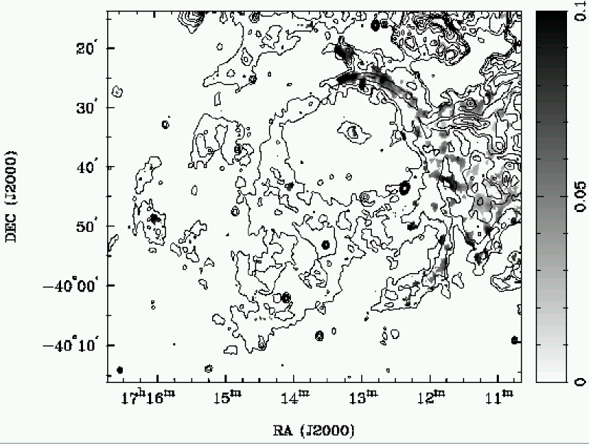
Figure 6: Fractional polarization for G347.3–0.5 at 1.4 GHz overlaid with the total intensity image over the whole SNR region. The grayscale is saturated to show regions with low values and units are of fractional polarization. The total intensity contours are: 0.5, 1, 2, 3, 5, 7, 10, 30 $\times$ 8 mJy beam^-1. At the location of Arc 1, the magnetic field appears to be most ordered and the polarized intensity follows the total intensity in this region.

We found significant linear polarization towards the western shell of G347.3–0.5. In Figure 6 we show the fractional polarization towards the SNR at 1.4 GHz. The mean fractional polarization is $\sim 5$% at 1.4 GHz and $\sim 10\%$ at 2.4 GHz, calculated by dividing the sum of polarized intensity by the sum of total intensity. The polarized intensity is strongest towards Arc 1, up to 12% at 1.4 GHz and 30% at 2.5 GHz, where it clearly follows the arc-like distribution of the total intensity. There is weaker ($<6$%), diffuse polarized emission from Arc 2. The polarized emission towards the rest of the western SNR region is patchy and diffuse, with no particular correlation with the radio continuum, implying that the magnetic field is not very highly ordered there and that most of the remnant has a high degree of depolarization. There is almost no polarization detected towards the rest of the SNR, with exception of a few small regions, e.g., towards the center region and the eastern SNR shell.

The multi-channel continuum capability of the ATCA can be used to derive the rotation measure (RM) across the observing bandwidth, caused by the Faraday rotation. Using the frequencies within 1.4 and 2.4 GHz bandwidths, we get RM values towards Arc 1 of $>+100$ rad m^-2. Our observed uncertainty in RM, $\Delta{\rm RM}\sim 20$ rad m^-2, implies an uncertainty in the intrinsic polarization position angle $\Delta\phi_{0}\sim\Delta{\rm RM}c^{2}/\nu^{2}\sim 1$ rad, when extrapolated from the RM measured within each band. Furthermore, we are unable to calculate the RM between the 1.4 and 2.4 GHz bands, because these observations have different wavelengths and angular resolution, and are thus subject to very different depolarization and Faraday rotation effects by foreground ionized gas (e.g., Gaensler et al., 2001). Thus we are unable to determine the intrinsic orientation of polarization from the available data.

4 Spectral Variations Across G347.3–0.5

Recently, Uchiyama, Aharonian & Takahashi (2003) presented a study of Chandra observations towards the northwestern rim of G347.3–0.5. In their spectral analysis of individual spectra from field 1 they infer that the photon index is same in diffuse and bright SNR regions. However, for their spectral fitting they used a blank sky observations for the background subtraction and varying column density for diffuse and bright regions. We also tried using blank sky observations for the background subtraction and found no difference in spectral fit results from the fitting using the background region from field 1. We also found that leaving column density as a free parameter for each individual spectrum results in very close photon index values. As explained in an earlier section ($\S$ 2.2), the possible variation in column density across the northwestern shell of the SNR seems unlikely; our use of a uniform value for $N_{\rm H}$ accounts for the difference in spectral indices between our work and that of Uchiyama, Aharonian & Takahashi (2003).

We produced two summed spectra, one for the bright and one for the faint SNR regions in field 1, which we fitted with power law and SRCUT models. The results from the fit are summarized in Table 2. The spectrum from bright regions has $\Gamma\sim 2.10$, while the spectrum from the faint regions has $\Gamma\sim 2.53$. When fitting the SRCUT model we froze again the radio spectral index to the global remnant value of 0.6 and left the normalization as a free parameters. The resuting rolloff frequency for the bright regions was $\nu_{rolloff}\sim 6.3\times 10^{17}$ Hz and for the faint regions was $\nu_{rolloff}\sim 1.2\times 10^{17}$ Hz. The radio flux at 1 GHz estimated by SRCUT of $S_{\nu}\sim 4.2$ Jy for the bright regions and $S_{\nu}\sim 2.9$ Jy for the faint regions is broadly consistent with that measured from our radio data, which gives us confidence in this approach.

These results, as well as those from fitting the individual spectra, imply that the fainter SNR regions have a steeper photon index and lower rolloff frequency than the bright regions. Thus, our data suggest that acceleration of particles to higher energies is more efficient in the brighter regions, perhaps because of the higher magnetic field in those regions. Another possibility is that electrons in the fainter regions are older, i.e., they could be produced in bright regions and then lose energy diffusing away from their origin.

5 High-resolution Comparison of X-ray and Radio Data

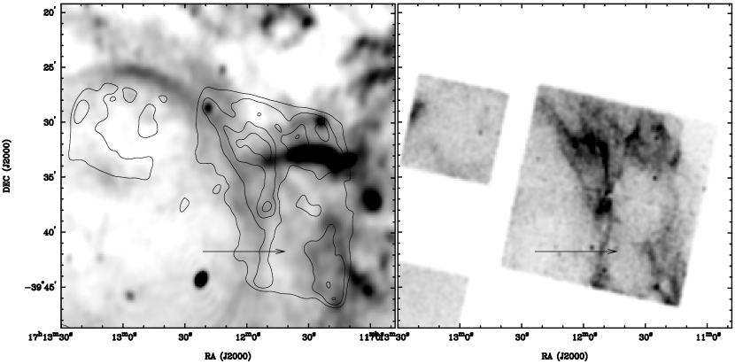
Figure 7: (left) 1.4 GHz greyscale image of the nortwestern SNR region overlaid with the Chandra contours convolved to the resolution of 1.4 GHz image of 47″. Contour levels are: 1, 2, 3 and 4 $\times 10^{-5}$ counts arcsec² s^-1. (right) 2″-resolution Chandra image of the nortwestern SNR region in the right panel. In both panels the arrow marks a profile cut region shown on Figure 9.

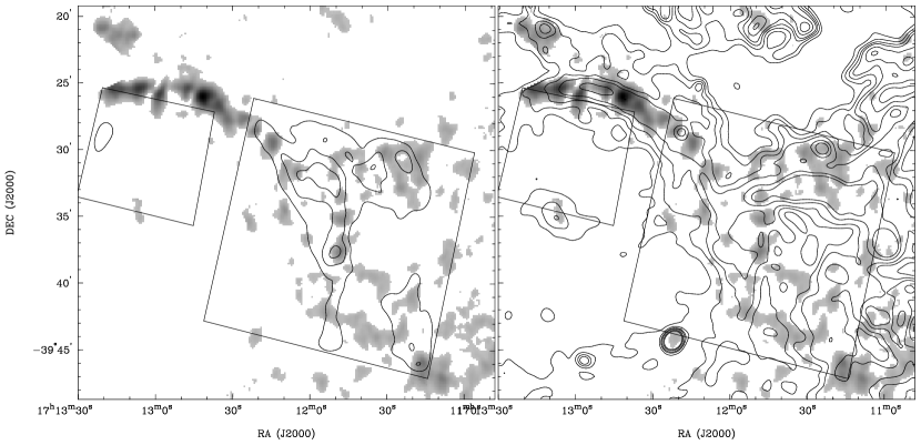
Figure 8: 1.4 GHz greyscale image of the polarized intensity towards the nortwestern SNR region overlaid in the left panel with the Chandra contours (convolved to the resolution of 1.4 GHz image of 47″) at 2, 3 and 4 $\times 10^{-5}$ counts arcsec² s^-1 levels, and with the 1.4 GHz continuum contours at 0.5, 1, 1.5, 2, 3 and 4 $\times 10^{-2}$ Jy. The squares are outlining the edges of the Chandra detectors.

Using our high-resolution radio and X-ray images we are able for the first time to address the correlation between the radio and X-ray morphology in a great detail. The Chandra and ATCA images of field 1 are overlaid in Figure 7 (left panel); we do not compare closely emission in field 2 because the radio emission is extremely weak there and shows no obvious structure. The Chandra image of the field 1 is shown smoothed to resolution of 2″  (right panel), as well as convolved to the resolution of 1.4 GHz ATCA image of 47″ (contours in the left panel). If the same population of electrons is responsible for the synchrotron emission in both the radio and X-ray band, one would expect similar morphology in these two bands, as appears to be the case for SN 1006 (Allen, Petre, & Gotthelf, 2001; Dyer et al., 2001). The correlation between the radio and X-ray images of G347.3–0.5 is not perfect, as noted from the ASCA data (Slane et al., 1999). Most notable is the lack of X-ray emission along the well-defined inner radio ring and the lack of radio emission from the southwestern peak present in the X-ray image — these regions were not imaged by us with Chandra so we compare ATCA and ROSAT images in Figure 5. However, the broad morphological agreement between the nonthermal X-ray and radio emission from field 1, and Arc 1 in particular (Figure 7), provides strong evidence that efficient particle acceleration is occurring in the northwestern part of the SNR. Arc 2 shows mostly diffuse emission, but a bright filament is present in the radio image which does not have a counterpart in the X-ray image. The nonthermal radio nature of Arc 2 was questioned by Ellison, Slane, & Gaensler (2001) due to its proximity to a region of thermal emission from the adjacent H ii region. Indeed, we find that this region has a large uncertainty in the radio spectral index, which implies confusion by the surrounding material. The X-ray spectrum of Arc 2 is clearly nonthermal; we found no indications of thermal X-ray emission towards this region. Furthermore, the polarized intensity in this region, shown in Figure 8, shows emission from Arc 2 which morphologically resembles X-ray data rather than the radio data. That implies that Arc 2’s radio emission is at least partially nonthermal.

The expected relation of radio and synchrotron X-ray morphology in an evolved, complex object like G347.3–0.5 is not simple. While we expect radio and X-ray emitting electrons to be born in the same shock waves, their subsequent evolution can vary greatly, because of different diffusive properties and the factor of 30,000 greater radiative lifetime for a 1 GHz-radiating electron compared to a 1 keV-radiating one. In fact, an electron radiating its peak synchrotron power in 1 keV photons has a half-life against synchrotron losses of

$$t_{1/2}=5.0\times 10^{4}B_{\mu{\rm G}}^{-3/2}\left({h\nu\over{1\ {\rm keV}}}\right)^{-1/2}\ {\rm yr}$$ (1)

where we have averaged over electron pitch angles. (Losses to inverse-Compton scattering from the cosmic microwave background (CMB) dominate for $B<3.2\ \mu$G, the field strength with the energy density of the CMB, so the maximum lifetime is about 8600 years for 1-keV-emitting electrons.) In a simple single shock wave, we might then expect radio and X-ray synchrotron emission to appear at the same location, with X-ray emission disappearing a shorter distance behind the shock. Such a morphology is evident in SN 1006 (Long et al., 2003) and in parts of RCW 86 (Rho et al., 2002). If the magnetic field is quite inhomogeneous, as we propose below, the lifetime of an individual electron will also depend strongly on the mean magnetic field along its particular diffusive trajectory. Furthermore, weak shocks may accelerate electrons to radio-emitting but not X-ray-emitting energies, so we should not be surprised to find radio emission without X-ray counterparts. Finally, X-rays can be absorbed by intervening gas at much lower column densities than would be required for free-free absorption of radio emission. In general, while we would hope to find at least some shock-like (thin linear) structures in X-rays and radio, there may not be an extremely close correspondence overall between the two bands.

Figure 9 shows profiles through the most prominent linear feature seen in both radio and X-ray, a thin filament at the inner edge of Arc 1. It is apparent that the turn-on of radio and X-rays is nearly coincident (we recall that the resolution of the radio image is 47″), while the radio emission extends considerably further than the X-rays. The width of the X-ray filament is about 40″ (1.2 pc at a distance of 6 kpc). If the leading edge of the structure is in fact a shock seen close to edge on, the X-ray width could result from synchrotron losses in a $3\ \mu$G field if the relativistic electrons are convected downstream (i.e., in the plane of the sky) at the modest velocity of about 140 km s^-1. As we argue below, the broadband spectrum of G347.3–0.5 can be explained if the magnetic-field structure consists of small regions with $B_{1}\sim 15\ \mu$G occupying about 1% of the volume, with a much lower field ($B_{2}<1\mu$G) occupying the rest. The mean field sampled by an electron would be fairly close to $B_{2}$, in this case, unless electrons were somehow trapped in the high-field regions. We therefore expect lifetimes of 1-keV-emitting electrons to be near the CMB limit of about 9000 yr, though in particular regions they could be much shorter. (An electron living all its life in $B_{1}$ would last only about 140 yr).

6 Origin of TeV Emission from G347.3–0.5

An earlier broad-band emission model for G347.3–0.5 by Ellison, Slane, & Gaensler (2001) implied that the IC mechanism was responsible for producing TeV emission from the remnant. The derived maximum electron energy of $E_{max}\sim 14\times 10^{12}$ eV falls below the “knee” energy, but they showed that in addition to efficient acceleration of electrons there can be efficient acceleration of ions (Fe⁺²⁶ in particular), whose maximum energy could reach the desired energy of $\sim 10^{15}$ eV. However, for this study only a single TeV flux measurement from the 3.8-m CANGAROO telescope was available. Most recently, Enomoto et al. (2002) published a $\gamma$-ray spectrum for G347.3–0.5 obtained with the new 10-m telescope, and suggested that the IC mechanism cannot produce the observed shape of the TeV spectrum. They modeled the TeV spectrum assuming pion-decay, which implies a higher particle density for the ambient medium than allowed by the X-ray emitting gas inside the SNR (Slane et al., 1999). If TeV emission is produced in regions outside the boundary of the SNR shock, where particles are upscattered through the diffusive acceleration process, the density values derived by Enomoto et al. (2002) from the pion-decay model might be plausible since the molecular cloud is so close to the remnant. In this case the bulk of TeV emission would have to originate in the cloud, somewhere beyond the SNR shell. Their pion-decay spectrum is inconsistent with EGRET observations (Butt et al., 2001; Reimer & Pohl, 2002), unless the proton spectrum has a cutoff below some energy, as also noted by Uchiyama, Aharonian & Takahashi (2003). This would result naturally if the protons must diffuse ahead of the shock to the molecular cloud, and if the diffusion coefficient increases with proton energy. In such a scenario only the highest-energy protons would reach the target, so that the pion-decay model would require an even higher target (molecular cloud) density, and demand even greater production efficiency of cosmic-ray protons at the shock. Uchiyama, Aharonian & Takahashi (2003) applied a two-zone model for the acceleration and diffusion of particles in an effort to explain the irregular morphology along the SNR limb. They considered the bright SNR filaments as locations where particles are accelerated, and the fainter regions where the electrons diffuse to after being accelerated. For a distance of 6 kpc, they derive a field strength of 50 $\mu$G, but require that this field be similar in the filamentary and diffuse emission regions. This then implies that the spectral cutoff in the diffuse emission regions is due to radiative losses while that in the filmants is due to diffusive escape of the particles. The resulting IC emission falls below the observed CANGAROO flux, thus requiering some other mechanism to produce the TeV emission. The IC mechanism was also rejected in the most recent study of ASCA data by Pannuti et al. (2003), because it required unrealistically low magnetic field filling factor (see next section). We wished to see, however, if our new Chandra data really supported ruling out the IC mechanism for the TeV emission.

6.1 The Broad-band Model

In Figure 10 we show measurements used to model the broad-band emission from G347.3–0.5. While the CANGAROO observations have poor angular resolution (for G347.3–0.5 observations estimated to be 0$\fdg$23; Enomoto et al., 2002), we shall assume that the TeV emission originates from particles in a broad region in the northwest of the SNR (see Muraishi et al., 2000), which includes the synchrotron-emitting regions. The similar radio and X-ray morphology towards the northwest suggests a common origin for the synchrotron-emitting particles at least in this part of G347.3-0.5. To match the spatial resolution of the CANGAROO data we produced a summed Chandra spectrum for the region covered by ACIS-I CCDs in field 1. The resulting unabsorbed X-ray flux in the 0.5–10.0 keV band is $\sim 1.3$$\times 10^{-10}$ erg cm^-2 s^-1. To measure radio flux densities, we convolved the radio images to 60″, which are then corrected for variations in the background level determined from the average of several areas around the region of interest. We obtained an integrated flux density from the region corresponding to field 1 of $6.7\pm 2.0$ Jy at 1.4 GHz, and $5.6\pm 1.7$ Jy at 2.4 GHz. The EGRET measurements are taken from Reimer & Pohl (2002), which used flux values from Hartman et al. (1999). The EGRET values correspond to the nearby source 3EG J1714–3857, which is either associated with G347.3–0.5 or else provides an upper limit to any such emission from the SNR. The CANGAROO measurements are taken from Enomoto et al. (2002).

We model the synchrotron and IC emission from G347.3–0.5 using a power law energy distribution modified by an exponential cutoff (e.g., Gaisser, Protheroe, & Stanev, 1998):

$$\frac{dN}{dE}=A_{e}~{}E^{-\sigma}exp\left[-\left(\frac{E}{E_{max}}\right)^{\alpha_{path}}\right],$$ (2)

where $A_{e}$ is the normalization factor, $\sigma$ is the index of the electron distribution and $E_{max}$ is the maximum energy of accelerated particles. We included additional parameter, $\alpha_{path}$, in the exponential function. This is a phenomenological parameter that allows for a broadening of cutoff, which accounts for variations in magnetic field from place to place, or in $E_{max}$, or both. A similar model was also used by Uchiyama, Aharonian & Takahashi (2003), or in a different form by Ellison, Slane, & Gaensler (2001). We use a steady-state model which assumes that the synchrotron and IC emission comes from a single population of relativistic electrons. Details of the model are given in Appendix A. The model yields estimates of the photon spectra produced by synchrotron and IC emission mechanisms in the $\nu F_{\nu}$ format:

$$\nu F_{\nu}(synch)=\frac{V_{E}}{4\pi D^{2}_{pc}}~{}f_{B}~{}\nu~{}P_{tot}(\nu,E),$$ (3)

$$\nu F_{\nu}(IC)=\frac{V_{E}}{4\pi D^{2}_{pc}}~{}E^{2}~{}\frac{dn_{\gamma}(\varepsilon_{\gamma})}{dt},$$ (4)

where $D_{pc}$ is the distance to the SNR in pc, $V_{E}$ is the electron emission volume (assuming a thin spherical shell geometry) given as (Ellison, Slane, & Gaensler, 2001):

$$V_{E}=f_{E}~{}\frac{4\pi}{3}(R_{O}^{3}-R_{I}^{3}).$$ (5)

$R_{O}$ and $R_{I}$ are the outer and inner shock radius respectively, and $f_{E}$ represents the fraction of the shell volume producing the emission seen from the northwestern SNR limb. The magnetic field filling factor $f_{B}$ in equation (3) corresponds to the fraction of the volume of IC-emitting electrons containing the magnetic field responsible for the synchrotron emission (e.g., Allen, Petre, & Gotthelf, 2001). $P_{tot}(\nu,E)$ and $\frac{dn_{\gamma}(\varepsilon_{\gamma})}{dt}$ are synchrotron and IC emissivities and are given in Appendix A.

Since the magnetic field strength $B$ and maximum particle energy $E_{max}$ cannot be determined independently from the synchrotron spectrum, we first modeled the CANGAROO data with an IC spectrum (treating the EGRET data as an upper limit for the flux detectable from the SNR) which depends only on $E_{max}$ (see Appendix A). In this way we determined the parameters for the electron number distribution: maximum electron energy $E_{max}=5$ TeV and particle index $\sigma=2.0$. We then varied the magnetic field strength, which is fixed by the ratio of peak emission frequencies $R_{\nu}$. An estimate good to about 25% is given by (see Appendix B)

$$B=9\times 10^{4}C_{\rm path}^{-1}R_{\nu}^{-1}{\rm G}.$$ (6)

The parameter $C_{\rm path}$ depends on the radio spectral index and on the parameter $\alpha_{\rm path}$ describing the breadth of the cutoff in the electron spectrum; by experimentation we found that for $\sigma=2,$ a value of $\alpha_{\rm path}=0.5$ described the X-ray data well. For these values, $C_{\rm path}=16$ which, with an estimate for $R_{\nu}\sim 10^{8.5}$, gives $B\sim 20\ \mu$G. We used our full model calculation for a more precise assessment and found that in order to match the shape of the X-ray spectrum we require $B\sim 15\,\mu$G. However, this would overpredict the synchrotron portion of the spectrum by a factor of 100. It is this problem that caused Enomoto et al. (2002) to rule out a synchrotron/IC model. But we can rescue such models by assuming that the magnetic field fills only a portion of the volume occupied by the IC-emitting electrons, and take a value of $\sim 0.01$ for the magnetic field filling factor $f_{B}$. This filling factor is given by (see Appendix B):

$$f_{B}=C(\sigma)R_{S}B^{(\sigma+1)/2}$$ (7)

where $R_{S}$ is the ratio between synchrotron and IC flux at a frequency in the power-law part of both spectra, and the values of $C(\sigma)$ are given in Appendix B. The values of the parameters used in the model are summarized in Table 3.

We note that using the SRCUT-type model (i.e., setting $\alpha_{path}=1$), our model gives parameters for the broad-band spectrum consistent with those of Pannuti et al. (2003), who derived high magnetic field ($\sim 150~{}\mu$G) and unrealistically low magnetic field filling factor ($\sim 10^{-3}$), the latter being the reason they rejected IC as a plausible mechanism for TeV emission production in G347.3–0.5. However, we find that the X-ray data seem to prefer slightly slower steepening of the cutoff than the sharp exponential cutoff. Thus our model with $\alpha_{path}=0.5$ results in different broad-band model parameters which are more reasonable from the physical point of view. Furthermore, our results illustrate the strong dependence of inferred parameters on the detailed model used to describe the synchrotron X-rays. This strong dependence means that particular parameter values obtained from this kind of broad-band fitting may be far less well-determined than their statistical uncertainties within a particular model may seem to indicate. Since our purpose here is mainly to illustrate that a synchrotron/IC broadband model is not ruled out by the data, we need only demonstrate that some reasonable model in this class can reproduce the observations, and we feel we have done so.

Thus, we find that, if the CANGAROO spectrum of G347.3–0.5 is correct, we have to decouple the electron emitting volume from the magnetic field volume to model the synchrotron spectrum with the parameters from the IC spectrum. We note that a magnetic field filling factor ($f_{B}$) value of $\sim 1$% seems very low, but MHD simulations do predict magnetic field enhancements in small-scale features produced by turbulence generated in SNR shocks (Jun & Jones, 1999). This is supported by the radio polarization maps of G348.3-0.5, which show that the magnetic filed in this SNR is very patchy, which could be, in part, due to the turbulent amplification. Also, this is the factor by which the volume occupied by magnetic field producing the bulk of the synchrotron emission is smaller than the volume occupied by ultrarelativistic electrons producing IC photons. In other words, the $15\ \mu$G magnetic field is confined to $\sim 1$% of the region from which the IC emission is emitted. This requires that the rest of the region has much lower magnetic field, $\sim 0.7\,\mu$G, in order not to exceed the total observed synchrotron emission from the SNR.

Our value for magnetic field is consistent with that calculated by Ellison, Slane, & Gaensler (2001), but our value for maximum energy of accelerated particles is factor of 3 lower. This is not surprising since $E_{max}$ is constrained by the TeV spectrum and their model was based on a single TeV measurement, which lies in the middle of the TeV spectrum and would thus push $E_{max}$ to the higher values. Using the rolloff frequency obtained from the SRCUT fit to field 1 spectra and our value for magnetic field, we get $E_{max}\sim 5.0$ TeV, using relationship

$$\nu_{rolloff}\approx 1.61\times 10^{16}\left(\frac{B}{10\mu{\rm G}}\right)\left(\frac{E}{10{\rm TeV}}\right)^{2}~{}{\rm Hz,}$$ (8)

which is the corrected version of the relationship reported in Reynolds & Keohane (1999) which contained a confusion of a factor of 0.29 between maximum and characteristic frequencies (see e.g., Pacholczyk, 1970). This value of $E_{max}$ is thus consistent with our model. In any case, given the uncertainties inherent in this kind of broad-band modeling of a highly inhomogeneous source, even a factor of 3 difference in inferred parameters should be regarded as rough consistency.

6.2 Maximum Energy of Accelerated Electrons

Our fitted value of $E_{max}$ of 5 TeV, with a magnetic field strength of $15\ \mu$G, gives a peak emitting frequency of $\nu_{ms}\sim 2\times 10^{15}$ Hz. This frequency is low enough to put significant constraints on shock-acceleration models producing the electron spectral cutoff by radiative losses. Simple estimates of the cutoff energy (e.g., Reynolds, 1998) in which the electron scattering mean free path is a constant factor $\eta\geq 1$ times the gyroradius give

$$E_{max}\sim 20\ \eta^{-1/2}\left(B\over{15\ \mu{\rm G}}\right)^{-1/2}u_{8}\ {\rm TeV}$$ (9)

where the shock normal is parallel to the mean upstream magnetic field, and

$$E_{max}\sim 20\ \eta^{+1/2}\left(B\over{15\ \mu{\rm G}}\right)^{-1/2}u_{8}\ {\rm TeV}$$ (10)

where the shock normal is more nearly perpendicular. The only difference is in the $\eta$-dependence, due to more rapid acceleration in perpendicular shocks (Jokipii, 1987). Also, $u_{8}$ is the shock velocity in units of $10^{8}$ cm s^-1, and $B$ is the postshock field strength. The above estimate is weakly dependent on the assumption that the shock compression ratio $r$ is 4.

These expressions give a cutoff frequency

$$\nu_{ms}({\rm perp})\equiv 1.82\times 10^{18}E_{max}^{2}B=3\times 10^{16}\eta~{}u_{8}^{2}\ {\rm Hz}$$ (11)

for a perpendicular shock, and

$$\nu_{ms}({\rm par})=3\times 10^{16}\eta^{-1}~{}u_{8}^{2}\ {\rm Hz}$$ (12)

for a parallel shock. These frequencies are independent of the magnetic field strength, since $E_{max}\propto B^{-1/2}$

If the shock velocity in G347.3–0.5 is about 1000 km s^-1 (Ellison, Slane, & Gaensler, 2001), it is impossible to produce the observed low cutoff frequency in perpendicular shocks — the acceleration rate is too fast. If the shocks are parallel, larger $\eta$ will slow the acceleration rate and lower the cutoff frequency. For instance, if $u_{\rm sh}=900$ km s^-1, then $\eta\sim 10$ would produce our inferred cutoff frequency. In the quasilinear approximation, electron scattering is due to the amplitude of magnetic fluctuations $\delta B$ with wavelengths comparable to the electron’s gyroradius. In this picture, $\eta=(\delta B/B)^{-2}$. In strong turbulence, $\eta$ approaches 1 (Bohm limit). A value of 10 is often assumed for moderately strong ($\delta B/B\sim 0.3$) turbulence.

The issue of the nature of the cutoff has important implications for the acceleration of ions. If the electron spectrum is limited by radiative losses, the proton spectrum might extend to much higher energies, while any other cutoff mechanism for electrons should affect protons as well. We deduce that if the shocks accelerating the electrons producing synchrotron X-rays in G347.3–0.5 are largely parallel shocks with fairly high levels of MHD turbulence, then the rate of electron acceleration can balance the loss rate for electron energies around the 5 TeV cutoff we obtain from fitting the TeV photon spectrum, and we cannot constrain any turnover in the accelerated proton spectrum. If the shocks do not have these properties, or if the acceleration is due to some other process altogether, we should expect that the proton spectrum also cuts off around 5 TeV.

Thus, assuming that protons are accelerated in the same manner as electrons, we can use the same particle distribution for electrons and protons (i.e., $\sigma=\sigma_{p}$ and $E_{max}=E_{max,p}$) to calculate total energy content of the relativistic electrons and protons (see Allen, Petre, & Gotthelf, 2001). We obtained a total electron energy of 3.7$\times 10^{46}$ erg and a total proton energy of 1.7$\times 10^{49}$ erg, which yields total particle energy that is significantly smaller than the SNR energy budget ($\sim 1-2\times 10^{51}$ erg). The total magnetic energy yields 4.6$\times 10^{46}$ erg for $B=15\mu$G and $f_{B}=0.01$, remarkably close to equipartition with electrons.

7 CONCLUSIONS

Chandra and ATCA observations of G347.3–0.5 have been used to investigate the SNR’s morphology and spectral properties with high angular resolution. The main results are summarized below.

The X-ray emission from the remnant is dominated by nonthermal power law emission, as found in previous observations. High resolution X-ray observations with Chandra reveal a complex morphology of the northwestern SNR region composed of bright filaments embedded in faint diffuse emission. Our spectral analysis implies that there are significant variations between the spectral properties of the fainter regions, which have steeper spectra ($\Gamma\sim 2.5$), and that of the bright regions, which have flatter spectra ($\Gamma\sim 2.1$).

To improve an estimate of the thermal emission in the SNR, we studied in particular the emission in the ACIS-S3 detectors which have the best response to the soft emission. We found a possible trace of thermal emission, but were unable to constrain its properties. No thermal component was detected in regions covered by the ACIS-I detectors.

Due to a complex environment the SNR is located in, we were unable to derive an accurate spectral index for radio emission. Using the ATCA data at 1.4 and 2.5 GHz we derived an approximate spectral index of the northwestern SNR region to be $0.50\pm 0.40$.

Significant linear polarization of $\sim 5$–10% is detected with the magnetic field being most ordered towards the northwestern SNR filament, where the linear polarization reaches 12–30%. The low mean value is comparable to that found in the historical shell remnants (see references in Reynolds & Gilmore, 1993), and is considerably smaller than often found in larger, older remnants. It is thus consistent with the otherwise surprising result that a remnant as large as G347.3-0.5 could have such strong shock acceleration.

We used the small scale morphology of Chandra data to identify possible regions of particle acceleration in the SNR. The X-ray morphology of the northwestern SNR region corresponds fairly well with the radio morphology, implying that the same population of electrons is responsible for the emission in both bands. We show that synchrotron/IC models cannot be ruled out for the broad-band spectrum, if we allow the possibility that the magnetic field is spatially inhomogeneous and enhanced in small regions. The data require a magnetic field of $\sim 15\mu$G occupying $\sim 1\%$ of the IC-emitting volume which is filled with relativistic electrons. The maximum energy of accelerated electrons is found to be $\sim 5$ TeV. The derived total electron and magnetic energies are close to equipartition in this model.

While non-thermal bremsstrahlung is not considered as a potential TeV emission mechanism because it would violate the limits on the thermal part of the bremsstrahlung emission from the SNR (Ellison, Slane, & Gaensler, 2001; Pannuti et al., 2003), there are objections for both IC and pion-decay processes. IC requires small magnetic field filling factor of nonthermal electrons ($f_{B}\sim 1\%$), while pion-decay requires extreme gas densities. While the very small filling factor may seem implausible, there is some observational evidence for such regions in G347.3–0.5. Future $\gamma$-ray telescopes with improved spatial resolution will help localize the TeV emission regions more precisely, enabling more accurate broad-band models to be derived.

Appendix A Synchrotron and Inverse Compton Models

The energy distribution in our synchrotron and inverse Compton (IC) models is taken to be a power law with an exponential cutoff (e.g Gaisser, Protheroe, & Stanev, 1998):

$$\frac{dN}{dE}=A_{e}~{}E^{-\sigma}exp\left[-\left(\frac{E}{E_{max}}\right)^{\alpha_{path}}\right],$$ (A1)

where $A_{e}$ is the normalization factor, $\sigma$ is the index of the particle distribution $E_{max}$ is the maximum energy of accelerated particles, and $\alpha_{path}$ is an empirical parameter allowing a broadening of the cutoff apparently required by observations (see e.g., Ellison, Slane, & Gaensler, 2001; Uchiyama, Aharonian & Takahashi, 2003).

The total synchrotron power radiated by a single electron is (e.g., Blumenthal & Gould, 1970)

$$p(\nu)=\frac{\sqrt{3}e^{3}B_{\bot}}{mc^{2}}\frac{\nu}{\nu_{c}}\int^{\infty}_{\nu/\nu_{c}}K_{5/3}(\xi)d\xi,$$ (A2)

where $\nu_{c}$ is the critical frequency given by

$$\nu_{c}=\frac{3eB_{\bot}}{4\pi m^{3}c^{5}}E^{2},$$ (A3)

$B_{\bot}$ is the magnetic field component perpendicular to the line of sight, and $K_{5/3}$ is the modified Bessel function of 5/3 order. The total power radiated by the population of electrons with the modified power law distribution $N(E)\equiv dN/dE$ is then

$$P_{tot}(\nu,E)=\int_{E_{min}}^{E_{max}}p(\nu)N(E)dE.$$ (A4)

For the IC spectrum we follow the formulae of Baring et al. (1999). The probability that a photon with initial energy $\varepsilon_{s}m_{e}c^{2}$ will collide with an electron of energy $\gamma_{e}=(E_{kin}-m_{e}c^{2})/m_{e}c^{2}$ and upscatter to the energy $\varepsilon_{\gamma}m_{e}c^{2}$ is given in the general case with the Klein-Nishina cross section as:

$$\sigma_{\rm K-N}(\varepsilon_{s},\gamma_{e};\varepsilon_{\gamma})=\frac{2\pi r_{0}^{2}}{\varepsilon_{s}\gamma_{e}^{2}}\left[2q~{}log_{e}q+1+q-2q^{2}+\frac{\delta_{e}^{2}q^{2}(1-q)}{2(1+\delta_{e}q)}\right],$$ (A5)

where $r_{0}=e^{2}/(m_{e}c^{2})$ is the electron radius, $\delta_{e}=4\varepsilon_{s}\gamma_{e}$ is a parameter that controls the importance of photon recoil and Klein-Nishina effects (Blumenthal & Gould, 1970), and $q$ is given as:

$$q=\frac{\varepsilon_{\gamma}}{\delta_{e}(\gamma_{e}-\varepsilon_{\gamma})},~{}~{}~{}0\geq q\geq 1.$$ (A6)

We take the photon field to be the cosmic microwave background (CMB) radiation, which has the spectral distribution of a blackbody at temperature of $T=2.73$ K:

$$n_{\gamma}(\varepsilon_{s})=\left(\frac{\varepsilon_{s}^{2}}{\pi^{2}\lambda_{c}^{3}}\right)\left(\frac{1}{e^{\varepsilon_{s}/\Theta}-1}\right)$$ (A7)

where $\Theta=\frac{kT}{m_{e}c^{2}}$, and $\lambda_{c}=\hbar/(m_{e}c)$ is the Compton wavelength. The IC emissivity is then

$$\frac{dn_{\gamma}(\varepsilon_{\gamma})}{dt}=c\int N_{e}(\gamma_{e})d\gamma_{e}\int n_{\gamma}(\varepsilon_{s})d\varepsilon_{s}\sigma_{\rm K-N}(\varepsilon_{s},\gamma_{e};\varepsilon_{\gamma}),$$ (A8)

where $N_{e}(\gamma_{e})\equiv dN/dE$ is the electron energy distribution. We have ignored other sources of seed photons for two reasons. First, in typical SNR environments the energy density of the local IR/optical radiation field is an order of magnitude or less than the CMB (Gaisser, Protheroe, & Stanev, 1998). While no emission in IRAS (Infrared Astronomical Satellite) images can be clearly associated with G347.3–0.5, an upper limit for the flux at 100$\mu$m can be estimated by taking all emission within the remnant boundaries. This gives about 450 Jy, or a mean intensity of about 0.16 Jy arcmin^-2, implying in the source an energy density $\nu u_{\nu}\sim 0.01$ eV cm^-3. This upper limit is far smaller than that of the CMB (0.26 eV cm^-3). Upper limits from the shorter-wavelength IRAS bands are even smaller than this. Second, the Klein-Nishina parameter $\delta_{e}$ is $\sim 10^{-2}$ for our 5 TeV electrons, meaning that the scattering cross-section is essentially the Thompson cross-section. For $\delta_{e}>1,$ the cross section begins to drop substantially due to Klein-Nishina suppression. This corresponds to photon wavelengths shortward of about 50 $\mu$m. So mid-to near-IR and optical seed photons would contribute substantially less to the IC emission, even if their energy densities were comparable to that of the CMB. We are thus justified in neglecting IR and higher photon fields in calculating the inverse-Compton emission from G347.3–0.5.

Appendix B Magnetic Field and Its Filling Factor

For a simple homogeneous source filled with relativistic electrons and magnetic field (with a filling factor $f_{B}$), we can write down simple relations between the synchrotron emission and inverse Compton emission from CMB seed photons. We consider spectra plotted as $\nu F_{\nu}$, so that both components rise with the same slope $1-\alpha$ (where $\alpha$ is radio spectral index) to peaks at frequencies $\nu_{ps}$ and $\nu_{pi}$, respectively. Since Compton upscattering increases scattered photon energies by a factor $\sim 2(E/m_{e}c^{2})^{2}$, a photon at the peak of the 2.73 K CMB spectrum with frequency $5.6\times 10^{10}$ Hz emerges at a frequency $\nu_{i}=1.7\times 10^{23}E^{2}$ Hz (with electron energy $E$ in erg). Now electrons with energy $E_{m}$ radiate the peak of their synchrotron radiation (SR) spectrum at a frequency $\nu_{m}=1.82\times 10^{18}E_{m}^{2}B$ (e.g., Pacholczyk, 1970). However, the peak of the resulting $\nu F_{\nu}$ spectrum is not necessarily at $\nu_{m}$. The delta-function approximation to the single-electron synchrotron emissivity, integrated over our modified exponentially cut off electron spectrum, gives a volume emissivity $j_{\nu}\propto\nu^{-\alpha}\exp(-(\nu/\nu_{m})^{\alpha_{\rm path}/2})$. The function $\nu j_{\nu}$ has a maximum at

$$\nu_{ps}=\left({3-\sigma}\over\alpha_{\rm path}\right)^{2/\alpha_{\rm path}}\nu_{m}\equiv C_{\rm path}\nu_{m}.$$ (B1)

For $\alpha_{\rm path}=1,$ $\nu_{p}=\nu_{m},$ but if $\alpha_{\rm path}<1,$ the increased broadening of the turnover moves the peak in $\nu j_{\nu}$ to higher frequencies, more so for flatter electron spectra (lower $\sigma$). (For $\sigma=2$ and $\alpha_{\rm path}=0.5,C_{\rm path}=16.$) We can then use the observed ratio of peak inverse-Compton frequency to peak synchrotron frequency $R_{\nu}\equiv\nu_{pi}/\nu_{ps}$ to solve for the magnetic field:

$$B=9\times 10^{4}C_{\rm path}^{-1}\left({\nu_{pi}\over\nu_{ps}}\right)^{-1}\ {\rm G}\equiv 9\times 10^{4}C_{\rm path}^{-1}R_{\nu}^{-1}\ {\rm G}.$$ (B2)

We can write down the ratio of synchrotron to inverse Compton emissivity at a given frequency (assuming a power law electron spectrum and neglecting Klein-Nishina effects, as is appropriate below the peak frequencies) from, e.g., Pacholczyk (1970); Rybicki & Lightman (1979), for the case of a thermal photon distribution at temperature $T$

$${j_{\nu}(SR)\over j_{\nu}(IC)}={c_{j}KB^{1+\alpha}\nu^{-\alpha}\over K\left(m_{e}c^{2}\right)^{\sigma-1}\left(2\pi r_{0}^{2}\right)\left(hc\right)^{-2}\left(kT\right)^{(\sigma+5)/2}F(\sigma)\left(h\nu\right)^{-\alpha}}$$ (B3)

where $K=A_{e}c^{\sigma+1}$ (so $dN/dE=KE^{-\sigma}$ far below the cutoff). Here $r_{0}$ is the classical electron radius, $h$ is Planck’s constant, and $c_{j}=c_{5}(\alpha)(1.25\times 10^{19})^{\alpha}$ in the notation of Pacholczyk (1970) ($c_{5}\sim 10^{-23}$ where cgs units are used throughout). Also,

$$F(\sigma)={\sigma^{2}+4\sigma+11\over\left(\sigma+3\right)^{2}(\sigma+5)(\sigma+1)}2^{\sigma+3}\Gamma_{f}\left({{\sigma+5}\over 2}\right)\zeta\left({{\sigma+5}\over 2}\right)$$ (B4)

where $\Gamma_{f}(z)$ is the complete gamma-function and $\zeta(z)$ is the Riemann zeta-function (see, e.g., Abramowitz & Stegun, 1965). This can be reduced to

$${j_{\nu}(SR)\over j_{\nu}(IC)}=7.92\times 10^{-8}\ {c_{j}B^{1+\alpha}\left(m_{e}c^{2}\right)^{\sigma-1}\over\left(kT\right)^{(\sigma+5)/2}F(\sigma)h^{(\sigma-1)/2}}.$$ (B5)

Inserting $T=2.73$ K for the cosmic microwave background, we obtain finally

$${j_{\nu}(SR)\over j_{\nu}(IC)}\equiv\left[C(\sigma)\right]^{-1}B^{1+\alpha},$$ (B6)

defining $C(\sigma)$ for later convenience we have $C(2.2)=6.8\times 10^{-14}$, $C(2.0)=2.1\times 10^{-14}$, and $C(1.7)=3.6\times 10^{-15}$.

Now the emitting volume of synchrotron radiation may be smaller than that of inverse Compton radiation, if the magnetic field occupies a fraction $f_{B}\leq 1$ of the volume. Then the ratio of SR to IC fluxes is smaller by a factor $f_{B}$. Including this factor and inverting equation (B5) above, we obtain

$$f_{B}=C(\sigma){F_{\nu}(SR)\over F_{\nu}(IC)}B^{-(1+\alpha)}.$$ (B7)

Estimates based on similar considerations (but for $f_{B}\equiv 1$) were obtained by Aharonian & Atoyan (1999). These results reproduce the results of detailed model fitting to within factors of 25% for $B$ and 2 for $f_{B}$.

Table 1: Parameters of the total and polarized intensity ATCA images at 1.4 GHz and 2.5 GHz.

Parameter	Values
$I_{1.4}$ FWHM beam	$46\farcs 3\times 36\farcs 2$, P.A.=$-3.8$
RMS noise in $I_{1.4}$	0.7  mJy beam-1
$Q_{1.4},U_{1.4}$ FWHM beam	$57\farcs 1\times 48\farcs 8$, P.A.=$-5.1$
RMS noise in $Q_{1.4},U_{1.4}$	0.2  mJy beam-1
$I_{2.5}$ FWHM beam	$24\farcs 7\times 17\farcs 9$, P.A.=$-$1.6
RMS noise in $I_{2.5}$	0.3  mJy beam-1
$Q_{2.5},U_{2.5}$ FWHM beam	$32\farcs 5\times 27\farcs 5$, P.A.=$-$3.1
RMS noise in $Q_{2.5},U_{2.5}$	0.3  mJy beam-1

Table 2: Results from the power law and SRCUT models fit to the summed Chandra spectra of G347.3–0.5 from bright and faint regions in field 1, with the 90% confidence ranges.

Parameter	Bright	Faint	Bright	Faint
	POW	POW	SRCUT	SRCUT
$N_{\rm H}$ ($10^{21}$ cm-2)	$7.7^{+0.2}_{-0.3}\times 10^{21}$ cm-2		$7.7\times 10^{21}$ cm-2
$\Gamma$/$\nu_{rolloff}$ (Hz)	$2.10^{+0.04}_{-0.03}$	$2.53^{+0.07}_{-0.07}$	$6.3^{+0.8}_{-0.6}\times 10^{17}$	$1.2^{+0.3}_{-0.4}\times 10^{17}$
$F_{X}$/$S_{\nu}$ ( erg cm-2 s-1/Jy)	$1.12^{+0.01}_{-0.03}$$\times 10^{-10}$	$2.65^{+0.07}_{-0.13}$$\times 10^{-11}$	$4.2^{+0.4}_{-0.2}$	$2.9^{+0.6}_{-0.4}$
$\chi^{2}_{red}$/dof	0.99/1077		1.00/1078

Table 3: Parameters used for modeling broad-band emission from G347.3–0.5 with synchrotron and IC mechanism.

Model Parameters	Values
Derived
Maximum electron energy, $E_{max}$	5.0${}_{-0.2}^{+0.1}$ TeV
Electron spectral index, $\sigma$	2.0${}_{-0.04}^{+0.05}$
Broadening factor, $\alpha_{path}$	0.5${}_{-0.02}^{+0.03}$
Electron normalization, $A_{e}$	5.5${}_{-0.1}^{+0.1}$$\times 10^{-32}$
Magnetic field strength, $B$	15${}_{-0.03}^{+0.05}$ $\mu$G
$B$ filling factor, $f_{B}$	0.010${}^{-0.003}_{+0.002}$
Fixed
SNR volume, $V_{E}$	4.9$\times 10^{59}$  cm-3
Emission filling factor, $f_{E}$	0.16
Outer SNR radius, $R_{O}$	40 pc
Inner SNR radius, $R_{I}$	34 pc
SNR distance, $D_{pc}$	6.3 kpc
reduced $\chi^{2}$/ degrees of freedom	1.55/338

Figure 4: Representative ACIS spectra from Chandra observations of G347.3–0.5 and the residuals for the best-fit model. The top spectrum is extracted from one of the brightes regions in SNR, marked with a star in Figure 2, and the bottom spectrum is from one of the faint regions marked with two stars in Figure 2.

Figure 9: Profile cut through Arc 1 from 1.4 GHz data (dash-dotted line) and Chandra data (solid line) marked in Figure 7.

Figure 10: Model of the broad-band emission from G347.3–0.5. The model shows estimates of the photon spectra associated with synchrotron and IC emission (see text).

References

- Abramowitz & Stegun (1965) Abramowitz, M., & Stegun, I. 1965, Handbook of Mathematical Functions (New York: Dover)
- Aharonian & Atoyan (1999) Aharonian, F. A. & Atoyan, A. M. 1999, A&A, 351, 330
- Allen, Petre, & Gotthelf (2001) Allen, G. E., Petre, R., & Gotthelf, E. V. 2001, ApJ, 558, 739
- Axford (1994) Axford, W. I. 1994, ApJS, 90, 937
- Baring et al. (1999) Baring, M. G., Ellison, D. C., Reynolds, S. P., Grenier, I. A., & Goret, P. 1999, ApJ, 513, 311
- Blandford & Eichler (1987) Blandford, R. & Eichler, D. 1987, Phys. Rep., 154, 1
- Blumenthal & Gould (1970) Blumenthal, G. R. & Gould, R. J. 1970, Reviews of Modern Physics, 42, 237
- Butt et al. (2001) Butt, Y. M., Torres, D. F., Combi, J. A., Dame, T., & Romero, G. E. 2001, ApJ, 562, L167
- Butt et al. (2002) Butt, Y. M., Torres, D. F., Romero, G. E., Dame, T. M., & Combi, J. A. 2002, Nature, 418, 499
- Crawford et al. (2001) Crawford, F., Gaensler, B. M., Kaspi, V. M., Manchester, R. N., Camilo, F., Lyne, A. G., & Pivovaroff, M. J. 2001, ApJ, 554, 152
- Dyer et al. (2001) Dyer, K. K., Reynolds, S. P., Borkowski, K. J., Allen, G. E., & Petre, R. 2001, ApJ, 551, 439
- Ellison, Slane, & Gaensler (2001) Ellison, D. C., Slane, P., & Gaensler, B. M. 2001, ApJ, 563, 191
- Enomoto et al. (2002) Enomoto, R. et al. 2002, Nature, 416, 823
- Frater, Brooks, & Whiteoak (1992) Frater, R. H., Brooks, J. W., & Whiteoak, J. B. 1992, Journal of Electrical and Electronics Engineering Australia, 12, 103
- Hartman et al. (1999) Hartman, R. C. et al. 1999,ApJS, 123, 79
- Hendrick & Reynolds (2001) Hendrick, S. P. & Reynolds, S. P. 2001, ApJ, 559, 903
- Gaensler et al. (2001) Gaensler, B. M., Dickey, J. M., McClure-Griffiths, N. M., Green, A. J., Wieringa, M. H., & Haynes, R. F. 2001, ApJ, 549, 959
- Gaisser, Protheroe, & Stanev (1998) Gaisser, T. K., Protheroe, R. J., & Stanev, T. 1998, ApJ, 492, 219
- Ginzburg (1957) Ginzburg, V. L., 1957, Prog. Elem. Particle Cosm. Ray Phys. 4, 339
- Katz-Stone & Rudnick (1997) Katz-Stone, D. M. & Rudnick, L. 1997, ApJ, 488, 146
- Killeen, Bicknell, & Ekers (1986) Killeen, N. E. B., Bicknell, G. V., & Ekers, R. D. 1986, ApJ, 302, 306
- Koyama et al. (1995) Koyama, K., Petre, R., Gotthelf, E. V., Hwang, U., Matsura, M., Ozaki, M., & Holt, S. S. 1995, Nature, 378, 255
- Koyama et al. (1997) Koyama, K., Kinugasa, K., Matsuzaki, K., Nishiuchi, M., Sugizaki, M., Torii, K., Yamauchi, S., & Aschenbach, B. 1997, PASJ, 49, L7
- Jokipii (1987) Jokipii, J.R., 1987, ApJ, 313, 842
- Jones & Ellison (1991) Jones, F. C. & Ellison, D. C. 1991, Space Science Reviews, 58, 259
- Jun & Jones (1999) Jun, B. & Jones, T. W. 1999, ApJ, 511, 774
- Lazendic et al. (2003) Lazendic, J. S., Slane, P. O., Gaensler, B. M., Plucinsky, P. P., Hughes, J. P., Galloway, D. K., & Crawford, F. 2003, ApJ, 593, L27
- Long et al. (2003) Long, K. S., Reynolds, S. P., Raymond, J. C., Winkler, P. F., Dyer, K. K., & Petre, R. 2003, ApJ, 586, 1162
- Mastichiadis & de Jager (1996) Mastichiadis, A. & de Jager, O. C. 1996, A&A, 311, L5
- Muraishi et al. (2000) Muraishi, H. et al. 2000, A&A, 354, L57
- Pacholczyk (1970) Pacholczyk, A.G. 1970, Radio Astrophysics (San Francisco: Freeman)
- Pannuti et al. (2003) Pannuti, T. G., Allen, G. E., Houck, J. C., & Sturner, S. J. 2003, ApJ, 593, 377
- Pfeffermann & Aschenbach (1996) Pfeffermann, E. & Aschenbach, B. 1996, Röntgenstrahlung from the Universe, eds. Zimmermann, H.U., Trümper, J., and Yorke, H., MPE Report 263, 267
- Prigozhin et al. (2000) Prigozhin, G. Y., Kissel, S. E., Bautz, M. W., Grant, C., LaMarr, B., Foster, R. F., Ricker, G. R., & Garmire, G. P. 2000, Proc. SPIE, 4012, 720
- Reimer & Pohl (2002) Reimer, O. & Pohl, M. 2002, A&A, 390, L43
- Reynolds & Chevalier (1981) Reynolds, S. P. & Chevalier, R. A. 1981, ApJ, 245, 912
- Reynolds & Gilmore (1993) Reynolds, S. P. & Gilmore, D. M. 1993, AJ, 106, 272
- Reynolds (1998) Reynolds, S. P. 1998, ApJ, 493, 375
- Reynolds & Keohane (1999) Reynolds, S. P. & Keohane, J. W. 1999, ApJ, 525, 368
- Rho et al. (2002) Rho, J., Dyer, K. K., Borkowski, K. J., & Reynolds, S. P. 2002, ApJ, 581, 1116
- Rybicki & Lightman (1979) Rybicki & Lightman 1979, Radiative processes in astrophysics (New York: Wiley-Interscience)
- Sault & Wieringa (1994) Sault, R. J. & Wieringa, M. H. 1994, A&AS, 108, 585
- Sault, Staveley-Smith & Brouw (1996) Sault, R. J., Staveley-Smith, L., & Brouw, W. N. 1996, A&AS, 120, 375
- Sault, Bock & Duncan (1999) Sault, R. J., Bock, D. C.-J., & Duncan, A. R. 1999, A&AS, 139, 387
- Sault & Killeen (2001) Sault, R. J. & Killeen, N., 2001, in Miriad Users Guide (Sydney: Australia Telescope National Facility)
- Shklovsky (1953) Shklovsky, I. S., 1953, Dokl. akad. Nauk. SSSR, 91, 475
- Slane et al. (1999) Slane, P., Gaensler, B. M., Dame, T. M., Hughes, J. P., Plucinsky, P. P., & Green, A. 1999, ApJ, 525, 35
- Slane et al. (2001) Slane, P., Hughes, J. P., Edgar, R. J., Plucinsky, P. P., Miyata, E., Tsunemi, H., & Aschenbach, B. 2001, ApJ, 548, 814
- Tanimori et al. (1998) Tanimori, T. et al. 1998, ApJ, 497, L25
- Townsley et al. (2000) Townsley, L. K., Broos, P. S., Garmire, G. P., & Nousek, J. A. 2000, ApJ, 534, L139
- Townsley et al. (2002) Townsley, L. K., Broos, P. S., Nousek, J. A. & Garmire, G. P. 2002, Nucl. Instrum. Methods Phys. Res. A, in press
- Uchiyama, Takahashi, & Aharonian (2002) Uchiyama, Y., Takahashi, T., & Aharonian, F. A. 2002, PASJ, 54, L73
- Uchiyama, Aharonian & Takahashi (2003) Uchiyama, Y., Aharonian, F. A. & Takahashi, T. 2003, A&A, 400, 567