Power Spectrum Normalisation and the Non-Gaussian Halo Model

Abstract

The normalisation of the matter power spectrum, $\sigma_{8}$, is an essential ingredient to predict the phenomenology of the low redshift universe. It has been measured using several methods, such as X-ray cluster counts, weak lensing and the cosmic microwave background, which have yielded values ranging from 0.7 to 1.0. While these differences could be due to systematic effects, they could also be due to physics beyond the standard $\Lambda$CDM model. An obvious possibility is the presence of non-Gaussian initial fluctuations in the density field. To study the impact of non-Gaussianity on each of these methods, we use a generalised halo model to compute cluster counts and the non-linear power spectrum for non-Gaussian models. Assuming scale invariance, the upper-limits on non-Gaussianity from the WMAP CMB experiment correspond to roughly a 4% shift in $\sigma_{8}$ as measured from cluster counts and about 2% shift through weak lensing. This is not enough to account for the current internal and mutual discrepancies between the different methods, unless non-Gaussianity is strongly scale dependent. A comparison between future X-ray surveys with a two fold improvement in cluster mass calibration and future cosmic shear surveys with 400 deg² will be required to constrain non-Gaussianity on small scales with a precision matching that of the current CMB constraints on larger scales. Our results argue for the presence of systematics in the current cluster and cosmic shear surveys, or to non-standard physics other than non-Gaussianity.

1 Introduction

In the inflation-driven $\Lambda$CDM paradigm, the initial fluctuations are assumed to obey Gaussian statistics. Current observations of the cosmic microwave background (CMB) of galaxy clustering and of galaxy clusters are consistent with this hypothesis (eg. Verde et al., 2001; Gaztañaga and Wagg, 2003). However, models with non-Gaussian initial conditions have been proposed and are not yet ruled out by observations (see Avila-Reese et al., 2003, and reference therein). These models include ones based on inflation theories with non-linearities of a single scalar field (Martin et al., 2000; Gangui et al., 2002) or with multi-fields (Peebles, 1999; Antoniadis et al., 1997; Linde and Mukhanov, 1997; Bernardeau and Uzan, 2002), or on cosmological defects (Turok and Spergel, 1990; Avelino et al., 1998).

In this paper, we study how non-Gaussian initial conditions can affect the determination of $\sigma_{8}$, the normalisation of the matter power spectrum on 8 $h^{-1}$ Mpc scales. This normalisation is an essential ingredient to predict the phonemenology of the low redshift universe and has been measured using several methods. The recent CMB measurements with WMAP (Spergel et al., 2003) yield a constraint on the normalisation of $\sigma_{8}=0.9\pm 0.1$ (68%CL). The abundance of galaxy clusters depends strongly on $\sigma_{8}$ and yields values in the range of $\sigma_{8}=0.7$-0.8 (eg. Pierpaoli et al., 2003) for $\Omega_{m}\approx 0.3$. Weak lensing by large-scale structure, or ’cosmic shear’, provides a direct measurement of mass fluctuations and has recently been detected and measured (see Refregier, 2003; Van Waerbeke and Mellier, 2003,  for recent reviews). The different cosmic shear surveys yield values of $\sigma_{8}$ in the range of $0.7-0.9$ for the same value of $\Omega_{m}$. The marginal discrepancies within and between these different techniques may be due to residual systematics, such as uncertainties in the mass-temperature of X-ray clusters, or the calibration of the shear in cosmic shear surveys. They could also be due to physics beyond the standard $\Lambda$CDM model, which has different effects on the various methods and surveys. In particular, non-Gaussianity appears as a prime candidate to explain discrepancies between the different methods. Cluster abundance and cosmic shear indeed both probe non-linear structures at low redshifts, but are sensitive to matter fluctuations on different scales. Non-Gaussianity may thus affect these two methods differently, while leaving the CMB power spectrum essentially unaffected. Reciprocally, it is interesting to establish whether the comparison between the different methods with present and future surveys may constrain non-Gaussianity.

To study the impact of non-Gaussianity on measurements of $\sigma_{8}$, we present a generalisation of the halo model (Ma and Fry, 2000; Seljak, 2000). Building on the work of Robinson and Baker (2000) for the mass function, Ma and Fry (2000) and Koyama et al. (1999) for the halo bias, and Navarro et al. (1996) and Avila-Reese et al. (2003) for the halo profiles, we compute the non-linear power spectrum for arbitrary non-Gaussian models. This allows us to compute the cluster temperature function and the cosmic shear statistics for these models. We then study whether a discrepancy in the determination of $\sigma_{8}$ from the different observational methods can be explained by non-Gaussianity. We also discuss how future surveys can be compared to set constraints on non-Gaussianity. The paper is organised as follows. In §2, we present the different non-Gaussian models and discuss how they are constrainted with current observations. In §3, we describe the non-Gaussian halo model. In §4, we study the effect of non-Gaussianity on the determination of $\sigma_{8}$ with the different methods. Our conclusions are summarised in §5.

2 Non-Gaussian Models

The statistics of the post-recombination linear density field $\rho$ are usually described by first forming the density contrast $\delta=(\rho-\overline{\rho})/\overline{\rho}$ with respect to the average matter density $\overline{\rho}=\langle\rho\rangle$ in the universe. We consider the probability distribution function (PDF) $p(\delta,M)$ of the density contrast $\delta$ smoothed with a spherical top-hat of radius $R$ corresponding to an enclosed mass $M=4\pi\overline{\rho}R^{3}/3$. It is defined so that

$$\int d\delta~{}p(\delta,M)=1,~{}~{}\int d\delta~{}p(\delta,M)\delta=\langle\delta\rangle=0.$$ (1)

The variance of the distribution is given by

$$\int d\delta~{}p(\delta,M)\delta^{2}=\langle\delta^{2}\rangle=\sigma^{2}(M)$$ (2)

and can be computed from the linear matter power spectrum $P_{\rm lin}(k)$ using

$$\sigma^{2}(M)=\int\frac{d^{3}k}{(2\pi)^{3}}~{}P_{\rm lin}(k)W^{2}(k,M),$$ (3)

where $W(k,M)=3(\sin kR/kR-\cos kR)/(kR)^{2}$ is the top-hat window function. The linear power spectrum is calculated using the transfer function from Bond and Efstathiou (1984).

To quantify the level of non-Gaussianity of the distribution, Robinson et al. (2000) have considered the excess probability $\alpha$ in the $3\sigma$ tail over that of a Gaussian PDF, i.e.

$$\alpha(M)=\frac{\int_{3\sigma(M)}^{\infty}d\delta~{}p(\delta,M)}{\int_{3\sigma(M)}^{\infty}d\delta~{}p_{\rm G}(\delta,M)}.$$ (4)

Another way of quantifying non-Gaussianity is the skewness

$$\mu_{3}(M)=\langle\delta^{3}\rangle=\int d\delta~{}p(\delta,M)\delta^{3}$$ (5)

To quantify non-Gaussianity from CMB measurements, several authors (eg. Komatsu et al., 2003; Verde et al., 2001) have considered the non-linear coupling $f_{NL}$ of the primordial (pre-recombination) potential field $\Phi$ to the Gaussian field $\Phi_{G}$, defined as

$$\Phi=\Phi_{G}+f_{NL}[\Phi_{G}^{2}-\langle\Phi^{2}\rangle].$$ (6)

This parametrisation is motivated by a class of inflation models. A conversion between $f_{NL}$ and the skewness $\mu_{3}$ of the (post-combination) density field can be derived using the results of Matarrese et al. (2000) and Verde et al. (2001). Current constraints from galaxy clusters (Avila-Reese et al., 2003; Robinson et al., 2000) yield $\alpha\la 4$ at 95%CL. As we will see in §4.1, the recent WMAP CMB measurement (Komatsu et al., 2003; Robinson et al., 2000) translates into $\alpha\la 1.6$ at 95%CL for $M\simeq 10^{14}M_{\odot}$.

As a special case, we consider scale free models, where the shape of the distribution is independent of the scale R. In this case, the PDF can be written as

$$p(\delta,M)=\sigma(M)^{-1}g\left(\sigma(M)^{-1}\delta\right),$$ (7)

where $g$ is a function which obeys

$$\int_{0}^{\infty}dx~{}g(x)=1,~{}~{}\int_{0}^{\infty}dx~{}xg(x)=0,~{}~{}\int_{0}^{\infty}dx~{}x^{2}g(x)=1,$$ (8)

so as to verify equations (1-2). For the Gaussian case,

$$g_{\rm G}(x)=(2\pi)^{-\frac{1}{2}}e^{-x^{2}/2}.$$ (9)

As an example of a scale invariant distribution, we consider the log-normal distribution which provides an adequate description of a range of non-Gaussian models based on non-linear or multi-field inflation and cosmic strings (Robinson and Baker, 2000). For this distribution,

$$g(x)=\frac{1}{\sqrt{2\pi}(x+x_{0})\beta}\exp\left[{-\frac{\ln^{2}\left(\frac{x+x_{0}}{\gamma}\right)}{2\beta^{2}}}\right],$$ (10)

where

$$x_{0}=\left(e^{\beta^{2}}-1\right)^{-\frac{1}{2}},~{}~{}\gamma=\left(e^{2\beta^{2}}-e^{\beta^{2}}\right)^{-\frac{1}{2}},$$ (11)

so as to enforce equation (8). The parameter $\beta$ controls the non-Gaussianity of the PDF and tends towards zero as the distribution becomes Gaussian. Figure 1 shows this distribution for several values of $\beta$ and corresponding values of $\alpha$.

Figure 1: Log-normal distribution for several values of the non-Gaussian parameter $\alpha$. The Gaussian case corresponds to $\alpha=1$, which is reached as $\beta\rightarrow 0$. For $\alpha=5.02$, $\alpha=9.61$, $\alpha=12.7$, and $\alpha=13.8$, the corresponding $\beta$ values are 0.2, 0.4, 0.6 and 0.8, respectively. For PDFs with a variance of 1 these correspond to $\mu_{3}$= 0.61, 1.32, 2.26 and 3.68.

3 Generalised Halo Model

A number of tools exist for modelling the growth of structure since inflation. On the largest scales, fluctuations in density are sufficiently small that their growth can be accurately modelled using linear theory. On small scales, however, the complex nonlinear interactions of gravitational in fall can, at present, only truly be modelled by using N-body simulation. These numerical simulations are however CPU intensive, making the exploration of parameter space prohibitively slow. To circumvent this, semi-analytic tools have been developed to provide fast and accurate fits to numerical simulations.

One such tool is the halo model (Ma and Fry, 2000; Seljak, 2000), which can be used to calculate the full non-linear power spectrum for a given cosmological model and has been shown to be in good agreement with high resolution numerical simulations. The halo model breaks the power spectrum into two parts: one that dominates on large scales and is determined by the clustering of halos of different masses, and a second term that is dominant on small scales and is determined by the density profile of the halos. The halo model thus requires three pieces of information: the mass-function of halos, the bias of halos compared to the background density field and the halo density profile. The halo model as described by Ma and Fry (2000) and Seljak (2000) calculates these three ingredients by assuming that the density perturbations are Gaussian. We show how this can be extended to include models that have non-Gaussian fluctuations.

3.1 Mass Function

Robinson and Baker (2000) have proposed a generalisation of the Press and Schechter (1974) formalism which provides a good fit to N-body simulations for a class of non-Gaussian models. In their formalism, the fraction of objects of a given mass $M$ or larger that collapse is calculated by integrating the PDF of the density fluctuations as

$$F(>M)=A\int_{\delta_{c}}^{\infty}P(\delta,M)d\delta,$$ (12)

where $A$ is a normalisation factor and $\delta_{c}$ is a critical over density which can be computed for arbitrary cosmologies using the results of Lacey and Cole (1993) and Eke et al. (1996). The mass function, defined as the number density of halos per unit mass, is then given by

$$\frac{dn}{dM}=\frac{\overline{\rho}}{M}\frac{d\nu}{dM}f(\nu),$$ (13)

where

$$f(\nu)=\left|\frac{dF}{d\nu}\right|$$ (14)

and

$$\nu=\frac{\delta_{c}}{\sigma(M)}.$$ (15)

The normalisation $A$ is chosen to ensure that all the matter is accounted for, so that

$$\frac{1}{\langle\rho\rangle}\int_{0}^{\infty}dM~{}M\frac{dn}{dM}=\int_{0}^{\infty}d\nu~{}f(\nu)=1.$$ (16)

For a scale invariant PDF (Eq. [7]), it is easy to show that equations (12) and (14) reduce to

$$f(\nu)=Ag(\nu),$$ (17)

with $A=\left[\int_{0}^{\infty}dx~{}g(x)\right]^{-1}$. This simple form reveals that the mass function at mass M provides a measure of the normalised PDF $g(x)$ at $x=\nu=\delta_{c}/\sigma(M)$. This assumes of course that the generalised Press-Schechter formalism is valid.

For the Gaussian case (Eq. [9]), we obtain the usual result

$$f_{\rm G}(\nu)=\sqrt{\frac{2}{\pi}}e^{-\nu^{2}/2},$$ (18)

with the usual normalisation factor $A=2$ prescribed by Press and Schechter (1974).

For the log-normal distribution (Eq. [10]), we obtain

$$f(\nu)=\frac{A}{\sqrt{2\pi}(\nu+x_{0})\beta}\exp\left[-\frac{\ln^{2}(\frac{\nu+x_{0}}{\gamma})}{2\beta^{2}}\right],$$ (19)

with

$$A=\left[{\rm erfc}\left(\frac{\ln(x_{0}/\gamma)}{\sqrt{2}\beta}\right)\right]^{-1},$$ (20)

where ${\rm erfc}$ is the complementary error function. Figure 2 shows the resulting differential mass function $dn/dM$ for this model at $z=0$, for several values of the non-Gaussian parameter $\alpha$. Non Gaussianity with $\alpha>1$ tends to increase the number of halos with $M\ga 10^{14}M_{\odot}$ and, to a smaller degree, to deplete halos with masses smaller than this limit. The high sensitivity of high mass halos to non-Gaussianity is expected since these halos probe the positive tail of the distribution. Throughout this paper we assume a standard $\Lambda$CDM model, with $\Omega_{m}=0.3,~{}\Omega_{\Lambda}=0.7,~{}h=0.7,~{}n=1\rm~{}and~{}\Gamma=0.21$. For this figure we adopted $\sigma_{8}=0.77$, but we will choose other values for this parameter depending on the data set considered.

Figure 2: Mass function at $z=0$ for the log-normal model with different values of the non-Gaussian parameter $\alpha$. The Gaussian case corresponds to $\alpha=1$, and the other values of $\alpha$ correspond to $\beta=0.01$, $0.05$, $0.2$, and $0.4$. For PDF’s with a variance of 1 these in turn correspond to $\mu_{3}$=0.03, 0.15, 0.61 and 1.32

3.2 Halo Bias

The bias parameter in the halo model describes how halos cluster compared to the underlying linear density field. Generalising the formalism of Mo and White (1996), Koyama et al. (1999) showed that the bias parameter for a general scale invariant PDF is given by

$$b(\nu)=1-\frac{1}{\delta_{c}}\left[1+\frac{d\ln f(\nu)}{d\ln\nu}\right].$$ (21)

Note that this expression satisfies the condition $\int d\nu~{}f(\nu)b(\nu)=1$, which is required to ensure that the linear power spectrum is recovered on large scales (see discussion in Seljak, 2000). For the scale invariant case, $f(\nu)$ is proportional to the PDF (see §3.1). The halo bias can therefore be thought of as a measure of the derivative of the PDF in this case. The measurement of halo bias, using the halo correlation function for instance, can thus be used to probe the PDF independently of the mass function.

For the Gaussian case (Eq. [18]), this reduces to the usual Mo & White result

$$b_{\rm G}(\nu)=1+\frac{\nu^{2}-1}{\delta_{c}}.$$ (22)

More accurate bias functions (eg. Jing, 1998) have been devised to provide better fits to N-body simulations, but they cannot be readily generalised to non-Gaussian models. Since we are only interested in the effect of non-Gaussianity relative to the Gaussian case, the above expression suffices for our purposes.

For the log-normal distribution, the bias function is

$$b(\nu)=1+\frac{1}{\delta_{c}}\frac{\nu}{\nu+x_{0}}\left[\frac{1}{\beta^{2}}\ln\left(\frac{\nu+x_{0}}{\gamma}\right)-\frac{x_{0}}{\nu}\right],$$ (23)

which does indeed go to Eq. [22] as $\beta$ tends towards zero. Figure 3 shows the bias as a function of mass for several values of $\alpha$. For skew-positive PDFs ($\alpha>1$), objects with low (high) masses are more (less) clustered compared to the Gaussian case.

Figure 3: Effect of $\alpha$ on the halo bias. The solid line shows the Gaussian case. We see that as we increase the level of fluctuations in the 3$\sigma$ tail, massive objects (high $\nu$) become less clustered, while less massive objects (low $\nu$) become more clustered.

3.3 Halo profile

We model the density profile of the halos as

$$\rho(r)=\rho_{s}u(r/r_{s}),~{}~{}u(x)=x^{-\mu}(1+x)^{\mu-3}$$ (24)

where $r_{s}$ is a characteristic radius. The inner slope $\mu$ must be less than 3 for convergence, and is equal to 1 in the case of a Navarro, Frenk & White (1996, NFW) profile and 1.4 in the case of a Moore et al. (1998) profile. We fix the normalisation $\rho_{s}$ so that the density contrast within the viral radius $r_{v}$ is $\delta_{v}=200$, i.e. so that $M=4\pi\overline{\rho}\delta_{v}r_{v}^{3}/3=4\pi\int_{0}^{r_{v}}dr~{}r^{2}\rho(r)$. This yields $\rho_{s}=\overline{\rho}\delta_{v}c^{3}U^{-1}(c)/3$ where we have defined the compactness parameter $c=r_{v}/r_{s}$, and

$$U(c)=\int_{0}^{c}dx~{}x^{2}u(x)=\frac{c^{3-\mu}}{3-\mu}~{}_{2}F_{1}(3-\mu,3-\mu;4-\mu;-c)$$ (25)

where ${}_{2}F_{1}$ is the hypergeometric function which can be evaluate numerically (Press et al., 1996). In the case of the NFW profile ($\mu=1$), this function reduces to $U(c)=\ln(1+c)-c/(1+c)$.

For the $\Lambda$CDM Gaussian model, a good fit to the non-linear power spectrum is given for an NFW profile ($\mu=1$) with the concentration parameter is chosen as (Cooray, 2000; Cooray et al., 2000)

$$c(M,z)=c_{*}(z)\left[\frac{M}{M_{*}(z)}\right]^{-h(z)}$$ (26)

where $c_{*}(M,z)\simeq 10.3(1+z)^{-0.3}$ and $h(z)\simeq 0.24(1+z)^{-0.3}$. Here $M_{*}(z)$ is the non-linear mass scale defined by $\nu(M_{*},z)=1$.

Avila-Reese et al. (2003) have used numerical simulations to measure the halo profiles in non-Gaussian models. For a model with $\alpha\approx 3$, they find an increase in the compactness parameter $c$ of about 20% compared to the Gaussian case for halos with masses in the range $10^{11}~{}\rm to~{}10^{15}~{}h^{-1}M_{\odot}$. They also find the inner slope to be steeper ($\mu\approx 1.6$) compared to the Gaussian NFW case ($\mu=1$).

More simulations would be needed to derive new scaling relations for halos in general non-Gaussian models. For our purposes, we use the use the NFW profile as a reference, but we also study the effect of changing the compactness and inner slope to those found by Avila-Reese et al. (2003).

3.4 Non-linear Power Spectrum

Ma and Fry (2000) and Seljak (2000) showed that the halo model provides an accurate prescription to compute the non-linear power spectrum for Gaussian models. In this formalism, the non-linear power spectrum $P(k)$ at a given redshift is written as

$$P(k)=P_{1}(k)+P_{2}(k),$$ (27)

where the 1-halo term is

$$P_{1}(k)=\int_{0}^{\infty}dM~{}\frac{dn}{dM}\left[\frac{\tilde{\rho}(k,M)}{\overline{\rho}}\right]^{2}$$ (28)

and the 2-halo term is

$$P_{2}(k)=\left[\int_{0}^{\infty}dM~{}\frac{dn}{dM}b(M)\frac{\tilde{\rho}(k,M)}{\overline{\rho}}\right]^{2}P_{\rm lin}(k).$$ (29)

In these expressions, $\tilde{\rho}(k,M)$ is the radial Fourier transform of the density profile (Eq. [24]) of a halo of mass $M$. The details of our implementation of the halo model can be found in Refregier and Teyssier (2002).

Figure 4 shows the effect of non-Gaussian initial conditions on the non-linear power spectrum. Non-Gaussianity is seen to affect transition scales $0.1\la k\la 3~{}h$ Mpc^-1 between the linear and the non-linear regime. The linear ($k\la 0.1h$ Mpc^-1) and strongly non-linear ($k\ga 3h$ Mpc^-1) are not significantly affected. Figure 5 shows the effect of varying the inner slope $\mu$ and the concentration parameter $c$ as indicated by the non-Gaussian simulations of Avila-Reese et al. (2003). Their suggested alteration of the concentration parameter by 20% (which we applied to all masses) tends to only slightly increase the power spectrum on small scales ($k\ga 3h$ Mpc^-1). On the other hand, the alteration of the inner profile $\mu$ by 60% increases the power spectrum significantly on these scales. Note however, that the mass dependence of $c(M)$ which we used as a reference (Eq. [26]) was chosen to reproduce the non-linear power spectrum in numerical simulations for an NFW profile ($\mu=1$). A selfconsistent fit to the non-linear power spectrum from non-Gaussian simulations would be needed to establish whether this effect is indeed so pronounced. In the following, we keep $c$ and $\mu$ unchanged from the Gaussian NFW case, but remain cautious in the interpretation of our model for the power spectrum on small scales.

Figure 4: Non-linear power spectrum at $z=0$ for several values of $\alpha$. The $\alpha=1$ Gaussian model (solid line) is a standard $\Lambda$CDM model with $\Omega_{m}=0.3$, $\Gamma=0.21$ and $\sigma_{8}=1.0$. Its decomposition into the 1-halo and the 2-halo terms are shown as long dashed lines.

Figure 5: Effect of the halo profile on the non-linear power spectrum. For $\alpha=3$, Avila-Reese et al. (2003) find an increase in the compactness parameter, $c_{ng}$ that is roughly 20$\%$ greater than that for the NFW profile, $c_{NFW}$. They also find the inner slope $\mu_{ng}\approx 1.6$ to be more cuspy for this level of non-Gaussianity, than that for the standard NFW profile $\mu_{NFW}=1$.

4 Power Spectrum Normalisation

4.1 Cosmic Microwave Background

Using the recent measurements from the WMAP mission, Spergel et al. (2003) found $\sigma_{8}=0.9\pm 0.1$ (68%CL). When combined with other CMB missions, galaxy surveys and Lyman alpha surveys, the authors find $\sigma_{8}=0.84\pm 0.04$ (68%CL). The CMB power spectrum provides a 2-point statistics of the matter fluctuations in the linear regime and is thus not affected by non-Gaussianity This is also true when it is combined with measurement of the galaxy power spectrum on linear scale, while assuming that the galaxy bias is scale independent. As a result, the determination of $\sigma_{8}$ based on fits to the CMB power spectrum (with and without galaxy surveys) is insensitive to non-Gaussianity.

The measurement of higher order statistics of CMB maps, however, does currently present tight constraints on the level of primordial non-Gaussianity. Using the WMAP measurements, Komatsu et al. (2003) were able to place limits on the non-Gaussian coupling defined in equation (6) of $-58<f_{NL}<134$ (95%CL). According to Matarrese et al. (2000,  figure 2), the upper limit corresponds to an upper limit on the skewness of the post-recombination density field (Eq. [5]) on scale of $M=10^{14}~{}M_{\odot}$ of $\mu_{3}\la 8.0\times 10^{-2}$, for a $\Lambda$CDM model with $\sigma_{8}=1$. For the log-normal distribution (Eq. [10]), this corresponds to $\alpha\la 1.6$ at the 95% confidence level. Note that this conversion assumes that the scale dependence of the non-Gaussianity is that of models given by equation (6).

4.2 X-ray Cluster Counts

Counting X-ray clusters is a direct probe of the mass function and provides a sensitive measure of $\sigma_{8}$. The main difficulty is to estimate the masses of X-ray selected clusters. The most reliable method to do so consists of measuring the X-ray temperature of the cluster and to use a mass-temperature ($M$-$T$) scaling relation. Using an M-T relation derived form hydrodynamical simulations, several groups have derived a value of $\sigma_{8}$ around 0.9 from measurements of the X-ray temperature function (see Pierpaoli et al., 2001,  and reference therein). More recently, the use of an observational $M$-$T$ relation led to a revision of $\sigma_{8}$ in the range $0.7$-$0.8$ (see eg. Pierpaoli et al., 2003; Seljak, 2001). The uncertainty in the $M$-$T$ relation is, at present, the largest source of uncertainty in cosmological parameter estimates using this method.

In order to study how the determination of $\sigma_{8}$ using this method is affected by non-Gaussianity, we consider the compilation of cluster temperature measurements presented by Pierpaoli et al. (2001). The catalogue consists of temperature measurements for 38 clusters taken using ROSAT and ASCA. The cluster temperatures range from $kT=3.5$ to $12$ keV, with those with temperatures greater than $7.5$ keV forming a volume limited sample. The resulting cumulative X-ray temperature function $n(>kT)$ from this compilation is shown in figure 6. To compute the cluster masses, Pierpaoli et al. (2001) have used the $M$-$T$ relation,

$$\frac{M(T,z)}{10^{15}h^{-1}M_{\odot}}=\left(\frac{T}{T_{*}}\right)^{\frac{3}{2}}\left(\Delta_{c}E^{2}\right)^{-\frac{1}{2}}\left(1-\frac{2\Omega_{\Lambda}}{\Delta_{c}}\right)^{-\frac{3}{2}},$$ (30)

where $T$ is the temperature in keV, and $E^{2}=\Omega_{m}(1+z)^{3}+\Omega_{\Lambda}+\Omega_{k}(1+z)^{2}$. The parameter $\Delta_{c}$ is the mean over density inside a virial radius and can be computed using the fitting functions given by Pierpaoli et al. (2001). In a later work, Pierpaoli et al. (2003) fit the observed temperature function using this relation and find $\sigma_{8}=0.77_{-0.04}^{+0.05}$ (68%CL).

Figure 6 also shows the predicted temperature function for different values of the non-Gaussian parameter $\alpha$. For the masses corresponding to $kT\ga 1$ keV (corresponding to $M\ga 3\times 10^{13}h^{-1}M_{\odot}$), a skew-positive PDF ($\alpha>1$) enhances the cluster counts (see Figure 2), the effect being more pronounced for larger temperatures. As a result, the determination of $\sigma_{8}$ from the X-ray cluster counts will be affected by non-Gaussianity. Figure 7 shows the value of $\sigma_{8}$ derived from a fit to the temperature function as a function of $\alpha$. Following Seljak (2001), we considered a fit to $n(>kT)$ at a single temperature $kT$, which we choose to be 4, 7, and 10 keV, in turn. For $kT\simeq 7$ keV and for the Gaussian case ($\alpha=1$), we find $\sigma_{8}\simeq 0.77$ in agreement with Pierpaoli et al. (2003) and Seljak (2001). The value of $\sigma_{8}$ required to fit the temperature function decreases as $\alpha$ increases. The effect is more pronounced for larger cluster temperatures, as expected.

Figure 6: Observed temperature function from the compilation of Pierpaoli et al. (2001). Also shown is the predicted temperature function for several values of the non-Gaussian parameter $\alpha$ and for $\sigma_{8}=0.77$.

Figure 7: Determination of $\sigma_{8}$ from a fit to the cluster temperature function as a function of the non-Gaussian parameter $\alpha$. Several temperatures $kT$ for the X-ray cluster counts are displayed.

4.3 Cosmic Shear

Weak lensing by large scale structure, or cosmic shear, provides a direct measure of the mass distribution in the universe (see Bartelmann and Schneider, 2001; Refregier, 2003; Van Waerbeke and Mellier, 2003, for recent reviews). This effect is based on the shear that intervening large-scale structures induce on the images of background galaxies. Several groups have now performed accurate measurements of cosmic shear (Jarvis et al., 2003; Hamana et al., 2002; Brown et al., 2003; Hoekstra et al., 2002; Refregier et al., 2002; Van Waerbeke et al., 2002; Bacon et al., 2002), which have been used to set constraints on cosmological parameters.

The 2-point cosmic shear statistics can be described by the weak lensing power spectrum (see Bacon et al. (2000) for conventions)

$$C_{\ell}=\frac{9}{16}\left(\frac{H_{0}}{c}\right)^{4}\Omega_{m}^{2}\int d\chi~{}\left[\frac{h(\chi)}{ar(\chi)}\right]^{2}P\left(\frac{\ell}{r},\chi\right),$$ (31)

where $\ell$ is the multipole moment, $\chi$ is the comoving radius, $r$ is the comoving angular-diameter distance, $a$ is the expansion parameter, and $H_{0}$ and $\Omega_{m}$ are the present value of the Hubble constant and matter density parameter, respectively. It can be computed for non-Gaussian models by using the halo-model approximation for the non-linear power spectrum $P(k,\chi)$ at a given comoving radius $\chi$, given in equation (27). The radial weight function is given by

$$h(\chi)=2\int_{\chi}^{\infty}d\chi^{\prime}~{}n(\chi^{\prime})\frac{r(\chi)r(\chi^{\prime}-\chi)}{r(\chi^{\prime})},$$ (32)

where $n(\chi)$ is the red shift distribution of galaxies and is normalised as $\int d\chi~{}n(\chi)=1$.

Figure 8 shows the weak lensing power spectrum for several values of $\alpha$. The galaxy redshift distributions was taken to be $n(z)\propto z^{2}\exp(-(z/z_{0})^{1.5})$ with $z_{0}=z_{m}/1.41$ and the median redshift was chosen to $z_{m}=1$ as suitable for several cosmic shear surveys. The cosmological parameters are those for our fiducial model given in §3.1 with $\sigma_{8}=1.0$. The linear power spectrum is also plotted for comparison and reveals that non-linear corrections are very important on scales $\ell\ga 10^{3}$. Non-Gaussianity has the most pronounced effect on intermediate scales $10^{2}\la\ell\la 10^{4}$, which is consistent with its effect on the 3D power spectrum (see figure 4). For $\alpha>1$, non-Gaussianity tends to increase the lensing power spectrum on these scales.

Figure 8: Weak lensing power spectrum $C_{\ell}$ for several values of the non-Gaussian parameter $\alpha$. The galaxy median redshift was assumed to be $z_{m}=1$. The Gaussian model ($\alpha=1$) is our fiducial $\Lambda$CDM model with $\sigma_{8}=1$.

In practice, it is often more convenient to consider the shear variance $\sigma_{\gamma}^{2}=\langle|\gamma|^{2}\rangle$ in randomly place circular cells of radius $\theta$. This is related to the shear power spectrum by

$$\sigma_{\gamma}^{2}=\frac{1}{2\pi}\int_{0}^{\infty}d\ell~{}C_{\ell}|W_{\ell}|^{2}$$ (33)

where $W_{\ell}=2J_{1}(\ell\theta)/(\ell\theta)$ is the Fourier transform of the cell aperture. The shear variance of the different non-Gaussian models is shown in figure 9. Also shown are recent measurements of the shear variance from different surveys with median galaxy redshifts in the range $0.8\la z_{m}\la 1$ (Brown et al., 2003; Refregier et al., 2002; Van Waerbeke et al., 2002; Bacon et al., 2002). The measurements are in rough agreement with each other and with the Gaussian $\Lambda$CDM case. Non-Gaussian models with $\alpha>1$ produce larger shear variances on scales $\theta\la 10^{\prime}$, i.e. on scales to which most surveys are sensitive. This is not surprising since this limit corresponds to the transition between the linear ($\theta\ga 10^{\prime}$) and non-linear ($\theta\la 10^{\prime}$) regimes for the shear statistics.

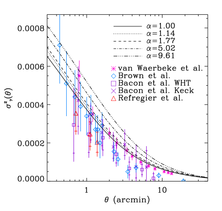
Figure 9: Shear variance $\sigma_{\gamma}^{2}(\theta)$ as a function of the circular cell radius. Both recent measurements (Brown et al., 2003; Refregier et al., 2002; Van Waerbeke et al., 2002; Bacon et al., 2002) and the predictions for the different non-Gaussian models (with $z_{m}=1$ and $\sigma_{8}=1$) are shown.

We therefore expect non-Gaussianity to affect the determination of $\sigma_{8}$ from current cosmic shear surveys. Figure 10 shows the value of $\sigma_{8}$ derived from the shear variance measured at different scales and with $z_{m}=1$, as a function of the non-Gaussian parameter $\alpha$. We see that if the universe is non-Gaussian with, say, $\alpha\approx 3$, the cosmic shear surveys (which assumed $\alpha$=1) would have overestimated $\sigma_{8}$ by about 5%. This shift is approximately unchanged if the galaxy redshift is set to $z_{m}$=0.6, as appropriate for shallower cosmic shear surveys (Jarvis et al., 2003; Hoekstra et al., 2002), which tend to find lower values of $\sigma_{8}$ than deeper ones (Brown et al. 2003; Refregier et al. 2002; Van Waerbeke et al. 2002; Bacon et al. 2002; see however Hamana et al. 2002). The discrepancy between shallower and some of the deeper surveys can therefore not be explained by non-Gaussianity.

As discussed in §3.3, the effect of non-Gaussianity depends on our assumption regarding the halo profile. We find that the bias in $\sigma_{8}$ is twice as pronounced if we use the modified profile suggested by Avila-Reese et al. (2003) instead of the NFW profile. Further high-resolution numerical simulations would be needed to resolve this theoretical uncertainty.

Figure 10: Determination of $\sigma_{8}$ from a fit to the cosmic shear variance $\sigma_{\gamma}^{2}(\theta)$ as a function of the non-Gaussian parameter $\alpha$. Several scales $\theta$ for the cosmic shear variance are displayed.

As expected, the effect of the non-Gaussian parameter, $\alpha$, depends on the scale being studied. On large angular scales, $\theta>10^{\prime}$, $\alpha$ has a very weak effect on the shear variance, which is as expected since these scales are still in the linear regime. The intermediate scales, $1^{\prime}\la\theta\la 10^{\prime}$, are the most affected by our non-Gaussian PDF, as can also be seen in figure 10. This is also consistent with the behaviour of the weak lensing power spectrum (figure 8) since these intermediate scales correspond to $10^{2}\la\ell\la 10^{3}$. On scales smaller than $\theta=1^{\prime}$, the variance from models with different $\alpha$ values no longer diverge from each other. This makes measurements on small angular scales less sensitive to variations in the PDF. On even smaller scales, corresponding to $\ell\ga 10^{4}$, the shift in the power spectrum changes sign, suggesting that on these scales the spread in shear variance of our models will decrease. Since lensing surveys do not probe these angular scales, we do not investigate this further.

4.4 Combined Constraints

As discussed in the previous sections, the determination of $\sigma_{8}$ from the CMB with and without galaxy surveys is insensitive to non-Gaussianity. On the other hand, cluster counts and cosmic shear are affected by non-Gaussianity, as can be seen in Figures 7 and 10. For $\alpha\la 5$, we find that the error in $\sigma_{8}$ made by ignoring non-Gaussianity can be approximated by

$$\Delta\sigma_{8}=\sigma_{8}^{G}-\sigma_{8}\simeq s(\alpha-1),$$ (34)

where $\sigma_{8}^{G}$ is the value derived by (wrongly) assuming a Gaussian model (i.e. corresponding to $\alpha=1$ in these figures). The slope $s$ and intercept values $\sigma_{8}^{G}$ are listed in table 1 for cluster counts and cosmic shear at different temperatures and angular scales. As is apparent from the figures and in the table, cluster counts are more sensitive ($s$ larger by a factor of about 2) than cosmic shear to non-Gaussianity. However, as noted above, the use of the Avila-Reese et al. (2003) halo profile instead of the NFW profile would tend to increase the cosmic shear slope $s$ by about a factor of 2, which would then nearly match that for cluster abundance. While this needs to be established by further numerical simulations, we will use the NFW slopes $s$ for cosmic shear as a reference but remember that they are lower limits.

Method	Scale	$s$	$\sigma_{8}^{G}$
cluster	4.0 keV	0.032	0.74
counts	7.0 keV	0.043	0.77
	10.0 keV	0.052	0.82
weak	0.5’	0.014	0.99
lensing	1.0’	0.017	0.99
	5.0’	0.019	0.99
	10.0’	0.015	0.99
	20.0’	0.011	0.99

Table 1: Fit parameters for the error $\Delta\sigma_{8}=\sigma_{8}^{G}-\sigma_{8}\simeq s(\alpha-1)$ made in the measurement of $\sigma_{8}$ if non-Gaussianity is ignored.

If we assume that the PDF shape is scale invariant over all scales, we have seen (see §4.1) that the recent WMAP skewness measurement imposes a constraint of $\alpha\la 1.3$ (68%CL). This limit corresponds to errors in $\sigma_{8}$ of $\Delta\sigma_{8}\simeq~{}0.02$ and 0.01, for cluster counts and cosmic shear respectively. These are significantly smaller to both the current uncertainties ($\Delta\sigma_{8}\approx~{}$0.05 and 0.1, respectively) and the discrepancy between the different methods and measurements ($\Delta\sigma_{8}\approx 0.3$). Thus, with this assumption, non-Gaussianity can not explain the internal and external discrepancies between these methods.

Note however that the above conclusion rests on an extrapolation from scales probed by WMAP ($\ell\la 1000$ corresponding to $\ga 25~{}h^{-1}$ Mpc comoving at decoupling) down to scales relevant for clusters and cosmic shear, 0.1 to 5.0 comoving $h^{-1}$Mpc. If we drop the assumption that the PDF is invariant over this large range of scales, the WMAP measurement no longer constrains the PDF relevant for these two latter techniques. In this case, we can attempt to reconcile the cluster and cosmic shear normalisations using non-Gaussianity. We find that this would require $\beta\simeq-0.4$. This level of negatively skewed PDF does not have a corresponding $\alpha$ parameter since the distribution does not have a 3$\sigma$ tail in this case. Such a negative skewness would be inconsistent with the observed shape of the temperature function (see figure 6) and of the shear variance (see figure 9).

Finally, we look at the level of accuracy future surveys need to reach in order to improve upon the current constraints on non-Gaussianity. Assuming scale invariance, we have shown that the current $1\sigma$ constraints set by WMAP correspond to uncertainties of $\Delta\sigma_{8}\approx 0.02$ for cluster counts and $\Delta\sigma_{8}\approx 0.01$ for cosmic shear. At present, cluster count measurements have $1\sigma$ uncertainties of $\Delta\sigma_{8}\approx 0.05$ which are dominated by an uncertainty in the normalisation $T_{*}$ of the $M$-$T$ relation of about 10%. This means that if the error on $\sigma_{8}$ from clusters is reduced by a factor of about 2 then they will be comparable to that arising from our lack of knowledge of the statistics of the density field. This will be achieved if the uncertainty in $T_{*}$ is reduced to about 4% in future surveys (see eg. Pierpaoli et al., 2003). Similarly, current lensing surveys of about 10 deg² have $1\sigma$ errors of $\Delta\sigma_{8}\approx 0.06$ (eg. Van Waerbeke et al., 2002) and scale as $\sqrt{A}$ where $A$ is the survey area. Lensing surveys will thus have to increase in sensitivity by a factor of about 6, and thus have areas of the order of 400 deg², before their measurement of $\sigma_{8}$ becomes sensitive to non-Gaussianity. Note, however, that it may be possible to probe primordial non-Gaussianity by studying higher order statistics of cosmic shear.

5 Conclusions

We have investigated the impact of non-Gaussian conditions on the determination of $\sigma_{8}$ via various observational methods. For this purpose, we have generalised the halo model to compute cluster statistics and the non-linear matter power spectrum. In passing, we noted that, for scale free non-Gaussian models, the halo mass function and bias provide a measure of the linear density PDF and of its derivative, respectively. The measurement of both of these statistics, therefore, provides an independent measure of the PDF and a test of its scale invariance.

The determination of $\sigma_{8}$ from the CMB power spectrum and from galaxy surveys in the linear regime is not sensitive to non-Gaussianity. On the other hand, the cluster X-ray temperature function tends to be enhanced at large temperatures ($T\ga 3$ keV) for skew-positive ($\alpha>1$) non-Gaussianity. If the primordial fluctuations are non-Gaussian and this is ignored, the determination of $\sigma_{8}$ from current X-ray cluster surveys would be overestimated by $\Delta\sigma_{8}\simeq 0.04(\alpha-1)$. This depends weakly on the typical temperature of the clusters. Cosmic shear statistics from current surveys probe the non-linear part of the matter power spectrum and are thus also sensitive to non-Gaussianity. Using the generalised halo model, we find that the matter power spectrum is enhanced by a factor of 2 on scales $0.1\la k\la 3~{}h\rm~{}Mpc^{-1}$ for skew-positive non-Gaussianity of $\alpha=5$. As a result, the cosmic shear power spectrum is also enhanced by a factor of 2 on scales $10^{2}\la\ell\la 10^{4}$. The error in $\sigma_{8}$ from current cosmic shear surveys if non-Gaussianity is ignored is $\Delta\sigma_{8}\simeq 0.02(\alpha-1)$. This behaviour depends weakly on the angular scale $\theta$ and on the galaxy redshift $z_{m}$. We also find that the nonlinear power spectrum, and therefore cosmic shear surveys may be sensitive to the halo profile. This, in turn, may be sensitive to the primordial density field and needs to be studied in more detail via high-resolution N-body simulations (see Avila-Reese et al., 2003).

The strongest upper limits on primordial non-Gaussianity are provided by the recent WMAP measurements and correspond to $\alpha-1\la 0.6$ (95% CL). Within this limit and assuming scale invariance, non-Gaussianity cannot explain the differences between the $\sigma_{8}$ values derived from different cosmic shear surveys and X-ray cluster catalogs. Dropping the assumption of scale invariance from the scales probed by WMAP to those probed by cluster counts and shear, non-Gaussianity would tend to decrease the derived values of $\sigma_{8}$ for both cosmic shear and cluster counts and thus would need to be very pronounced to explain the discrepancy. Specifically, a highly negatively skewed PDF with $\beta\approx-0.4$ (which does not have a corresponding $\alpha$) would be needed to resolve the discrepancy, but would not be compatible with the observed shape of the cluster temperature function and of the cosmic shear 2-point function. A comparison between future X-ray surveys with a two fold improvement in cluster mass calibration and future cosmic shear surveys with 400 deg² will be required to constrain non-Gaussianity on small scales with a precision matching that of the current CMB constraints on larger scales. Our results suggest that the discrepancies are either due to systematics in one or several of the methods or to non-standard physics other than non-Gaussianity.

References

- Antoniadis et al. (1997) Antoniadis, I., Mazur, P. O., and Mottola, E.: 1997, Physical Review Letters 79, 14
- Avelino et al. (1998) Avelino, P. P., Shellard, E. P. S., Wu, J. H. P., and Allen, B.: 1998, ApJ 507, L101
- Avila-Reese et al. (2003) Avila-Reese, V., Colin, P., Piccinelli, G., and Firmani, C.: 2003, ArXiv Astrophysics e-prints
- Bacon et al. (2002) Bacon, D., Massey, R., Refregier, A., and R.S., E.: 2002, ArXiv Astrophysics e-prints
- Bacon et al. (2000) Bacon, D. J., Refregier, A. R., and Ellis, R. S.: 2000, MNRAS 318, 625
- Bartelmann and Schneider (2001) Bartelmann, M. and Schneider, P.: 2001, Phys. Rep. 340, 291
- Bernardeau and Uzan (2002) Bernardeau, F. and Uzan, J.: 2002, Phys. Rev. D 66, 103506
- Bond and Efstathiou (1984) Bond, J. R. and Efstathiou, G.: 1984, ApJ 285, L45
- Brown et al. (2003) Brown, M. L., Taylor, A. N., Bacon, D. J., Gray, M. E., Dye, S., Meisenheimer, K., and Wolf, C.: 2003, MNRAS 341, 100
- Cooray (2000) Cooray, A.: 2000, Phys. Rev. D 62, 103506
- Cooray et al. (2000) Cooray, A., Hu, W., and Miralda-Escudé, J.: 2000, ApJ 535, L9
- Eke et al. (1996) Eke, V. R., Cole, S., and Frenk, C. S.: 1996, MNRAS 282, 263
- Gangui et al. (2002) Gangui, A., Martin, J., and Sakellariadou, M.: 2002, Phys. Rev. D 66, 83502
- Gaztañaga and Wagg (2003) Gaztañaga, E. and Wagg, J.: 2003, Phys. Rev. D 68, 21302
- Hamana et al. (2002) Hamana, T., Miyazaki, S., Shimasaku, K., Furusawa, H., Doi, M., Hamabe, M., Imi, K., Kimura, M., Komiyama, Y., Nakata, F., Okada, N., Okamura, S., Ouchi, M., Sekiguchi, M., Yagi, M., and Yasuda, N.: 2002, ArXiv Astrophysics e-prints
- Hoekstra et al. (2002) Hoekstra, H., Yee, H. K. C., and Gladders, M. D.: 2002, ApJ 577, 595
- Jarvis et al. (2003) Jarvis, M., Bernstein, G. M., Fischer, P., Smith, D., Jain, B., Tyson, J. A., and Wittman, D.: 2003, AJ 125, 1014
- Jing (1998) Jing, Y. P.: 1998, ApJ 503, L9+
- Komatsu et al. (2003) Komatsu, E., Kogut, A., Nolta, M. R., Bennett, C. L., Halpern, M., Hinshaw, G., Jarosik, N., Limon, M., Meyer, S. S., Page, L., Spergel, D. N., Tucker, G. S., Verde, L., Wollack, E., and Wright, E. L.: 2003, ApJS 148, 119
- Koyama et al. (1999) Koyama, K., Soda, J., and Taruya, A.: 1999, MNRAS 310, 1111
- Lacey and Cole (1993) Lacey, C. and Cole, S.: 1993, MNRAS 262, 627
- Linde and Mukhanov (1997) Linde, A. and Mukhanov, V.: 1997, Phys. Rev. D 56, 535
- Ma and Fry (2000) Ma, C. and Fry, J. N.: 2000, ApJ 543, 503
- Martin et al. (2000) Martin, J., Riazuelo, A., and Sakellariadou, M.: 2000, Phys. Rev. D 61, 83518
- Matarrese et al. (2000) Matarrese, S., Verde, L., and Jimenez, R.: 2000, ApJ 541, 10
- Mo and White (1996) Mo, H. J. and White, S. D. M.: 1996, MNRAS 282, 347
- Moore et al. (1998) Moore, B., Governato, F., Quinn, T., Stadel, J., and Lake, G.: 1998, ApJ 499, L5+
- Navarro et al. (1996) Navarro, J. F., Frenk, C. S., and White, S. D. M.: 1996, ApJ 462, 563
- Peebles (1999) Peebles, P. J. E.: 1999, ApJ 510, 523
- Pierpaoli et al. (2003) Pierpaoli, E., Borgani, S., Scott, D., and White, M.: 2003, MNRAS 342, 163
- Pierpaoli et al. (2001) Pierpaoli, E., Scott, D., and White, M.: 2001, MNRAS 325, 77
- Press and Schechter (1974) Press, W. H. and Schechter, P.: 1974, ApJ 187, 425
- Press et al. (1996) Press, W. H., Teukolsky, S. A., Vetterling, W. T., and Flannery, B. P.: 1996, Numerical Recipes in C, Cambridge University Press
- Refregier (2003) Refregier, A.: 2003, ArXiv Astrophysics e-prints
- Refregier et al. (2002) Refregier, A., Rhodes, J., and Groth, E. J.: 2002, ApJ 572, L131
- Refregier and Teyssier (2002) Refregier, A. and Teyssier, R.: 2002, Phys. Rev. D 66, 43002