Cosmological acceleration, varying couplings, and Lorentz breaking

Abstract

Many candidate fundamental theories contain scalar fields that can acquire spacetime-varying expectation values in a cosmological context. Such scalars typically obey Lorentz-violating effective dispersion relations. We illustrate this fact within a simple supergravity model that also exhibits the observed late-time cosmological acceleration and implies varying electromagnetic couplings.

I Introduction

An important question in present-day cosmology concerns the expansion history of our universe. Recent measurements indicating a late-time period of accelerated expansion [1] have been met with great interest. Possible theoretical explanations for this observation typically involve new fundamental physics including a cosmological constant [2], quintessence-type models [3] with one [4] or two [5] scalar fields, k-essence [6], and exotic equations of state like that of the generalized Chaplygin gas [7].

Other astrophysical observations claim evidence for a time-dependent fine-structure parameter [8]. Early speculations in the subject of varying couplings date back to Dirac’s large-number hypothesis [9]. Subsequent theoretical investigations have shown that a spacetime dependence of the fine-structure parameter arises naturally in candidate fundamental theories and is often accompanied by variations of other gauge or Yukawa couplings [10]. In light of these facts, a confirmation of the experimental observations and the search for realistic models that permit other particle-physics and cosmological predictions have assumed particular urgency [11]. In this context, studies along the lines of the Bekenstein model [12] and its generalizations have suggested dark matter and a cosmological constant [13], an ultra-light scalar field [14], and quintessence [15] as driving entities for a varying fine-structure parameter.

The presence of varying couplings implies a breaking of invariance under temporal or spatial translations. This can be seen as a special case of the violation of spacetime symmetries, which also include Lorentz and CPT invariance. In fact, time-dependent couplings typically affect these additional symmtries as well [16]. Note also that Lorentz and CPT breakdown has been suggested in a variety of approaches to fundamental physics. We mention string theory [17], spacetime foam [18, 19], nontrivial spacetime topology [20], loop quantum gravity [21], and noncommutative geometry [22]. Lorentz and CPT violation provides therefore another independent signature for an underlying theory.

Scalar fields are a common feature in all of the above contexts. This shows that scalars play a key role in the search for fundamental physics. It becomes therefore interesting to investigate cosmological expansion, varying couplings, and Lorentz violation within a single candidate fundamental model containing scalars. In the present work, we shall consider an $N=4$ supergravity model in four spacetime dimension. The model contains two scalar fields, an axion and a dilaton, with a potential that we model with mass-type terms. This framework, although not fully realistic in its details, incorporates many features expected to be present in an encompassing theory: the pure four-dimensional $N=4$ supergravity is a limit of the $N=1$ supergravity in 11 dimensions, which is contained in M theory.

The paper is organized as follows. Section II describes the basics of our model. In Sec. III, we demonstrate how, for a suitable range of parameters, a late-time period of accelerated cosmological expansion can arise in such a supergravity model. The associated variation of the fine-structure parameter and the electromagnetic $\theta$ angle is investigated in Sec. IV. Section V discusses the violation of Lorentz and CPT symmetry in the presence of spacetime-dependent scalars. A brief summary is contained in Sec. VI.

II Basics

The starting point for our investigation is an isotropic homogeneous flat $(k=0)$ Friedmann-Robertson-Walker universe with the usual line element

$$ds^{2}=dt^{2}-a^{2}(t)\;(dx^{2}+dy^{2}+dz^{2})\;,$$ (1)

where $a(t)$ denotes the scale factor and $t$ the comoving time. The assumption of flatness simplifies the analysis and seems justified in light of recent measurements [23].

In the present context, we are interested in physical effects past the formation of Hydrogen. We therefore neglect the energy-momentum contribution of radiation to the source of the Einstein equations. Galaxies and other matter are modeled in a standard way by the energy-momentum tensor of dust:

$$T_{\mu\nu}=\rho u_{\mu}u_{\nu}\;.$$ (2)

Here, $\rho$ is the energy density of the matter and $u^{\mu}$ is a unit timelike vector orthogonal to the spatial hypersurfaces, as usual.

In addition, our model contains two real scalar fields, an axion $A$ and a dilaton $B$, coupled to the electromagnetic field $F_{\mu\nu}$. The fields are described by the Lagrangian density ${\cal L}_{\rm sg}$ obeying

$$\kappa{\cal L}_{\rm sg} = -{\textstyle{{1}\over{2}}}\sqrt{g}R+\sqrt{g}({\partial_{\mu}A\partial^{\mu}A+\partial_{\mu}B\partial^{\mu}B})/{4B^{2}}$$ (4)

$$\qquad\!-{\textstyle{{1}\over{4}}}\kappa\sqrt{g}MF_{\mu\nu}F^{\mu\nu}-{\textstyle{{1}\over{4}}}\kappa\sqrt{g}NF_{\mu\nu}\tilde{F}^{\mu\nu}\;,$$

where

$$M = {{B(A^{2}+B^{2}+1)}\over{(1+A^{2}+B^{2})^{2}-4A^{2}}}\;,$$ (5)

$$N = {{A(A^{2}+B^{2}-1)}\over{(1+A^{2}+B^{2})^{2}-4A^{2}}}\;.$$ (6)

Here, $\tilde{F}^{\mu\nu}=\varepsilon^{\mu\nu\rho\sigma}F_{\rho\sigma}/2$ denotes the dual field-strength tensor and $g=-\det(g_{\mu\nu})$. For convenience, we rescale $\rho\rightarrow\rho/\kappa$ and $F^{\mu\nu}\rightarrow F^{\mu\nu}/\sqrt{\kappa}$ in what follows. Then, the gravitational coupling $\kappa$ does not appear explicitly in the equations of motion. Under the assumption that the dust arises through fermions uncoupled from the scalars $A$ and $B$ and with the identification of $F^{\mu\nu}$ with one of the graviphotons, this model fits into the framework of $N=4$ supergravity in four dimensions [24, 16].

The pure N=4 supergravity is known to be incomplete. For example, its spectrum differs from the observed particle species in nature, and the matter couplings of $F^{\mu\nu}$ are nonminimal. This latter issue can be avoided by gauging the internal SO(4) symmetry leading to a potential for the scalars that is unbounded from below [25]. However, besides additional fields, any realistic situation requires a stable vacuum. We are therefore led to a phenomenological approach and take the effective potential to be bounded from below. We further assume that the scalars remain effectively uncoupled from the matter. This may explicitly break the supersymmetry, but does not represent a problem phenomenologically.

To lowest order, we model the potentials for these scalars by quadratic self-interactions for the axion and dilaton parametrized by the coefficients $m_{A}$ and $m_{B}$, respectively. Then, our full Lagrangian density ${\cal L}$ reads:

$${\cal L}={\cal L}_{\rm sg}-{\textstyle{1\over 2}}\sqrt{g}(m_{A}^{2}A^{2}+m_{B}^{2}B^{2})+g_{\mu\nu}T^{\mu\nu}\;.$$ (7)

Note that $m_{A}$ and $m_{B}$ cannot be identified directly with the masses of $A$ and $B$ because of the non-canonical kinetic terms.

The next step is to determine the equations governing the evolution of the universe. Our above assumptions of matter dominance, homogeneity, and isotropy imply that we can neglect electromagnetic effects for the large-scale dynamics of the universe. We therefore set $F_{\mu\nu}=0$ for the moment. Moreover, the matter density $\rho$ and the scalars $A$ and $B$ are (like the scale factor $a$) functions of the comoving time $t$ only. Then, the respective $00$ and $jj$ components of the Einstein equations including the dust are given by:

$$6{{\dot{a}^{2}}\over{a^{2}}} = m_{A}^{2}A^{2}+m_{B}^{2}B^{2}+{{\dot{A}^{2}+\dot{B}^{2}}\over{2B^{2}}}+2\rho\;,$$ (8)

$$4{{\ddot{a}}\over{a}}+2{{\dot{a}^{2}}\over{a^{2}}} = m_{A}^{2}A^{2}+m_{B}^{2}B^{2}-{{\dot{A}^{2}+\dot{B}^{2}}\over{2B^{2}}}\;,\qquad$$ (9)

where the dot denotes a derivative with respect to the comoving time. The off-diagonal components are trivial.

The equations for the time evolution of the axion and the dilaton are obtained by variation of ${\cal L}$ with respect to $A$ and $B$, as usual:

$${{d}\over{dt}}\left({{a^{3}\dot{A}}\over{B^{2}}}\right) = -2a^{3}m_{A}^{2}A\;,$$ (10)

$$\quad{{d}\over{dt}}\left({{a^{3}\dot{B}}\over{B^{2}}}\right) = -2a^{3}m_{B}^{2}B-{{a^{3}}\over{B^{3}}}(\dot{A}^{2}+\dot{B}^{2})\;.$$ (11)

The above equations of motion for $A$ and $B$ imply that the energy contained in the scalars is conserved separately:

$$0 = a^{3}D_{\mu}\Theta^{\mu 0}$$ (12)

$$= {{d}\over{dt}}\left[{{a^{3}}\over{4B^{2}}}(\dot{A}^{2}+\dot{B}^{2})+{{a^{3}}\over{2}}(m_{A}^{2}A^{2}+m_{B}^{2}B^{2})\right]$$ (14)

$${}+{{3a^{2}\dot{a}}\over{2}}\left[{{1}\over{2B^{2}}}(\dot{A}^{2}+\dot{B}^{2})-m_{A}^{2}A^{2}-m_{B}^{2}B^{2}\right],$$

where $\Theta^{\mu\nu}$ denotes the symmetric energy-momentum tensor associated with the scalars $A$ and $B$. This essentially arises as a result of the fact that our model fails to contain interactions of the axion and the dilaton with the fermion dust. This is a phenomenologically reasonable assumption: energy exchange between the scalars and the dust can only be mediated by the electromagnetic field. However, the matter content of the universe is electrically neutral and stable against photodecay on macroscopic scales, which excludes the required rates of photon exchange.

As an immediate consequence of the above result, the energy-momentum tensor $T_{\mu\nu}$ of the dust is also covariantly conserved. This gives the equation ${d(\rho a^{3})}/{dt}=0$, which can be integrated to yield $\rho(t)=c_{\rm n}/a^{3}(t)$. Here, the integration constant $c_{\rm n}=\rho_{\rm n}a_{\rm n}^{3}$ is determined by the matter density $\rho_{\rm n}=\rho(t_{\rm n})$ and scale size $a_{\rm n}=a(t_{\rm n})$ of the universe at the present time $t_{\rm n}$.

Note that Eqs. (9) and (11) are four equations for the three unknown functions $a(t)$, $A(t)$, and $B(t)$. To demonstrate the dependency among them, one can proceed as follows. Multiplication of the first Einstein equation in (9) with $a^{3}$ and subsequent application of a time derivative eliminates the term containing $\rho$ by energy conservation. Moreover, with the aid of the equations of motion for the scalars in the form of Eq. (14), one can rearrange the remaining expression to obtain the second one of the Einstein equations in (9).

III Accelerated cosmological expansion

In this section, we investigate the solutions of the Eqs. (9) and (11), which govern the dynamics of our model. The two Einstein equations (9) imply

$$6{{\ddot{a}}\over{a}}=m_{A}^{2}A^{2}+m_{B}^{2}B^{2}-{{\dot{A}^{2}+\dot{B}^{2}}\over{B^{2}}}-\rho\;.$$ (15)

Thus, in a physical model at least one one of the parameters $m_{A}$ or $m_{B}$ must be nonzero to yield an accelerated expansion rate $\ddot{a}(t)>0$, as expected. This is also consistent with a previous analysis taking $m_{A}=m_{B}=0$: in this case, all equations of motion can be integrated analytically leading to the conventional decelerated expansion $\sim t^{2/3}$ of a matter-dominated universe in the present cosmological epoch [16].

In special situations in which $m_{A}$, or $m_{B}$, or both are nonzero, some analytical results can be obtained. These results together with some general comments on the spectrum of solutions can be found in Appendix A. However, for the present purposes numerical methods appear most promising for further progress. A phenomenologically interesting input-parameter set should minimize the deviation from experimental data. As a result of the nonlinearity and the complexity of the present system of differential equations, it appears difficult to find a global minimum. A numerical search has given a variety of parameter sets optimizing locally the departure from observations. One such set sufficient for our purposes is the following:

$$m_{A} = 2.7688\times 10^{-42}\,{\rm GeV}\;,$$ (16)

$$m_{B} = 3.9765\times 10^{-41}\,{\rm GeV}\;,$$ (17)

$$c_{\rm n} = 2.2790\times 10^{-84}\,{\rm GeV}^{2}\;,$$ (18)

$$a(t_{\rm n}) = 1\;,$$ (19)

$$A(t_{\rm n}) = 1.0220426\;,$$ (20)

$$\dot{A}(t_{\rm n}) = -8.06401\times 10^{-46}\,{\rm GeV}\;,$$ (21)

$$B(t_{\rm n}) = 0.016598\;,$$ (22)

$$\dot{B}(t_{\rm n}) = -2.89477\times 10^{-45}\,{\rm GeV}\;.$$ (23)

The numerical analysis also showed that there are two sets of solutions: one in which the scale factor $a(t)$ increases with time and another one in which the scale factor decreases. In what follows, we only consider the observationally relevant solution with $\dot{a}(t)>0$.

Our next step is to compare the solution determined by the parameters (23) with experimental data. Measurements show that the expansion of our universe is consistent with a flat “canonical” model containing nonrelativistic matter (dust) and a cosmological constant $\Lambda$. The parameters for this canonical model are inferred from observations of high-redshift supernovae [26]:

$$\Omega_{\rm M} = 0.30\pm 0.04\;,$$ (24)

$$\Omega_{\Lambda} = 0.70\pm 0.04\;,$$ (25)

$$H_{0} = (70\pm 4)\>{\rm km\!\cdot\!s^{-1}\!\cdot\!Mpc^{-1}}\;.$$ (26)

Here, $\Omega_{\rm M}$ and $\Omega_{\Lambda}$ are the respective energy densities associated with the matter and the $\Lambda$ term relative to the critical density $3{H_{0}}^{2}/\kappa$. The Hubble constant is denoted by $H_{0}$, as usual. To make contact with observations, we can therefore compare our solution determined by the input values (23) with the above canonical model (26). To allow only small deviations of the supergravity cosmology from the best-fit canonical model, we have chosen the variations in the parameters (26) to be somewhat smaller than the experimental errors [26]. We also take the variations of the relative energy densities $\Omega_{\rm M}$ and $\Omega_{\Lambda}$ to be constrained by $\Omega_{\rm M}+\Omega_{\Lambda}=1$, so that the canonical model yields a flat ($k=0$) universe for all parameters (26).

The supergravity cosmology leads to a value for the Hubble constant of $H_{0}\simeq 69\,{\rm km\!\cdot\!s^{-1}\!\cdot\!Mpc^{-1}}$ consistent with observations. The canonical model yields $t_{\rm n}=1.35\times 10^{10}\,{\rm yr}$ for the present age of the universe. Our supergravity cosmology implies a similar age of ${t_{\rm n}}=1.30\times 10^{10}\,{\rm yr}$.

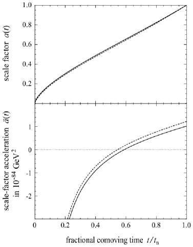
FIG. 1.: Time evolution of the scale factor $a(t)$ and its second derivative $\ddot{a}(t)$. The solid and dashed lines correspond to our supergravity universe and the canonical model, respectively. Note that for approximately the second half of its lifetime, the expansion of the universe is speeding up in both models.

Other features of the cosmological expansion are illustrated in Fig. 1. The upper panel shows the evolution of scale factor from the Big Bang to the present. The time dependence of the scale-factor acceleration $\ddot{a}(t)$ is depicted in the lower panel. The solid and the dashed lines refer to our supergravity cosmology and the canonical model, respectively. The fractional comoving time is determined by the corresponding $t_{\rm n}$ values of each model given in the previous paragraph. Note the recent accelerated expansion of the universe in both cosmologies at comparable rates.

Although the differences in scale-factor evolution between our and the canonical model seem relatively minor in Fig. 1, it is necessary to investigate whether these deviations are such that consistency with observations is maintained. Experimentally, the time dependence of the scale factor is inferred from luminosity and redshift measurements of distant cosmological objects. Conventionally, the luminosity observations are translated into a luminosity distance $D_{L}$ that can be expressed as a distance-modulus value $(m-M)$. In Fig. 2, $\Delta(m-M)_{\Omega=0}=(m-M)-(m-M)_{\Omega=0}$ is plotted as a function of redshift $z$. To emphasize the acceleration effects, we have subtracted the distance modulus $(m-M)_{\Omega=0}$ of an empty $(k=-1)$ non-accelerated universe with $a(t)=H_{0}t$ and $H_{0}=70\>{\rm km\!\cdot\!s^{-1}\!\cdot\!Mpc^{-1}}$. As before, the solid line corresponds to our supergravity model and the dashed line to the canonical model. The dotted line represents the empty universe. The shaded area corresponds to the parameter space (26). In the shown redshift region, which corresponds to the current observational range of $z\mathrel{\hbox to0.0pt{\lower 4.0pt\hbox{\hskip 1.0pt$\sim$}\hss}\raise 1.0pt\hbox{$<$}}1$, both models explain the supernovae data. At higher redshifts $z>1$, the models could in principle be distinguished by future experiments of this type.

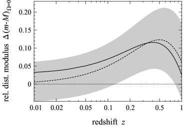
FIG. 2.: Distance modulus relative to an empty universe $\Delta(m-M)_{\Omega=0}$ versus redshift $z$. Our supergravity cosmology is represented by the solid line and the canonical model by the dashed line. The dotted line corresponds to the empty universe. The shaded region marks the parameter range (26).

Next, we briefly discuss the time evolution of the scalars $A(t)$ and $B(t)$. The values (23) lead to the comoving-time dependence of the axion and dilaton fields depicted in Fig. 3. For clarity, the value of $B(t)$ has been multiplied by a factor of ten. The scalars $A(t)$ and $B(t)$ vary significantly only in the early universe. At later times, they display a comparatively constant behavior, which is phenomenologically necessary because the axion and the dilaton determine the variation of the fine-structure parameter, which is tightly constrained experimentally. A more detailed discussion of this topic can be found in the next section.

We conclude this section with a few comments on two further quantities of interest. One of them is the equation-of-state parameter $w\equiv p_{\rm s}/\rho_{\rm s}$, where $p_{\rm s}$ denotes the pressure of the scalars and $\rho_{\rm s}$ their energy density. Figure 4 shows a plot of $w$ versus the fractional comoving time. Note that $w$ is significantly different from $-1$ only at early times. It follows that in the recent past the scalars affect the expansion of the universe essentially in the same way as a cosmological constant.

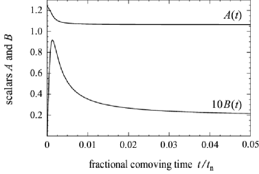
FIG. 3.: Time evolution of the scalars $A(t)$ and $B(t)$ at early cosmological times. In the recent past of our model universe, which is not shown here, $A(t)$ and $B(t)$ are essentially constant.

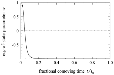
FIG. 4.: Time evolution of the equation-of state parameter $w$. At late times, $w\rightarrow-1$, so that the scalars essentially obey the cosmological-constant equation of state.

The second quantity of interest is the distribution of energy between the nonrelativistic matter and the scalars. In Fig. 5, the relative energy density of the dust, $\Omega_{\rm M}$, is plotted versus the fractional comoving time. The relative energy density $\Omega_{\rm S}$ associated with the scalars obeys $\Omega_{\rm M}+\Omega_{\rm S}=1$ in a flat universe, so that the shaded region corresponds to the time evolution of $\Omega_{\rm S}$. At late times, $\Omega_{\rm S}$ becomes the dominant energy component in our model. This behavior, which is characteristic for a conventional universe with positive $\Lambda$ energy, arises because the equation of state for the scalars approaches that of a cosmological constant. The supergravity cosmology exhibits an energy distribution differing from the conventional case only at early times: $\Omega_{\rm S}$ also dominates close to the Big Bang. However, we remind the reader that our simple model neglects important effects prior to the recombination time.

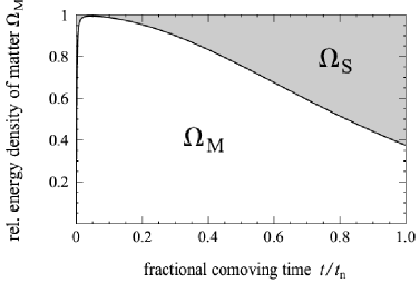
FIG. 5.: Relative energy density of matter $\Omega_{\rm M}$ versus fractional comoving time. The shaded area shows $\Omega_{\rm S}$, which corresponds to the energy associated with the axion-dilaton background. At late times, $\Omega_{\rm S}$ dominates, which parallels the cosmological-constant situation.

IV Varying couplings

In this section, we consider excitations of $F_{\mu\nu}$ in the axion-dilaton cosmology discussed above. In most experimental investigations, the spacetime regions involved are small on a cosmological scale, so that it is appropriate to work in local inertial frames. A few of the following results have been derived previously for the case $m_{A}=m_{B}=0$ [16]. However, we discuss them here anew, both for completeness and to emphasize qualitative differences to the present case.

The conventional electrodynamics Lagrangian density in a local inertial frame can be taken as

$${\cal L}_{\rm em}=-{{1}\over{4e^{2}}}F_{\mu\nu}F^{\mu\nu}-{{\theta}\over{16\pi^{2}}}F_{\mu\nu}\tilde{F}^{\mu\nu}\;.$$ (27)

We remind the reader that the $\theta$-angle term fails to contribute to the classical Maxwell equations as long as $\theta$ remains constant. Comparison with our supergravity model yields $e^{2}\equiv 1/M$ and $\theta\equiv 4\pi^{2}N$. Note that $M$ and $N$ are functions of the scalars $A$ and $B$. It follows that the time dependence of $A$ and $B$ in the supergravity cosmology induces a time variation of $e$ and $\theta$. Thus, in the present model the fine-structure parameter and the electromagnetic $\theta$ angle acquire related spacetime dependences in a general coordinate system.

In Fig. 6, the relative variation $(\alpha-\alpha_{\rm n})/\alpha_{\rm n}$ of the fine-structure parameter $\alpha=e^{2}/4\pi$ is plotted versus the fractional look-back time $1-t/t_{\rm n}$ to the Big Bang. Here, $\alpha_{\rm n}=1/137$ denotes the present value of the electromagnetic coupling. The solid line represents our supergravity model with the input (23). Also plotted is the recently reported Webb dataset [8] obtained from observations of high-redshift spectra. Both the supergravity cosmology and the data show a relative variation of $\alpha$ by parts in $10^{5}$. Although our model fails to provide a good match to the data, it does exhibit nonlinearities in $\alpha(z)$, a necessary feature to fit all experimental constraints.

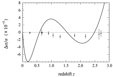
FIG. 6.: Relative time variation of the electromagnetic coupling versus fractional look-back time to the Big Bang. The present model with the parameters (23) is represented by the solid line. Also shown is the Webb dataset.

We mention that a generic choice of model parameters typically yields a much larger variation of $\alpha$, which can be understood as follows. The supergravity cosmology is governed by the coupled equations of motion for the scale factor $a(t)$ and the scalars $A(t)$ and $B(t)$. The observed value of the Hubble constant provides the experimental constraint $\dot{a}/a\sim 10^{-10}\;{\rm yr}^{-1}$. One would therefore expect that this is also the approximate variation of the axion-dilaton background. This value, however, is roughly six orders of magnitude larger than the scale for $\dot{\alpha}/\alpha$ suggested by the Webb data [8].

In a general phenomenological model involving some scalar field $\phi$, the difference in the scales for $\dot{a}/a$ and $\dot{\alpha}/\alpha$ is typically bridged as follows. One normally expands $\alpha(\phi)=\alpha_{\rm n}(1+\xi\phi)+\ldots$, which permits adjusting the parameter $\xi$ to obtain the desired order of magnitude for $\dot{\alpha}/\alpha$. Note that this normally introduces an additional scale into such a phenomenological model. In the present supergravity framework, however, the dependence of $\alpha$ on the scalars $A$ and $B$ is fixed, so that adjustable coefficients in the electromagnetic coupling are absent. The above discussion suggests that this is a critical issue in models with parameter-free interactions linking cosmological expansion and variation of couplings via the same scalar field(s).

V Apparent Lorentz violation

It is known that spacetime-varying couplings are typically associated with Lorentz violation [16]. We summarize this result first before further investigation. In the present context, Lorentz violation is exemplified by the modified Maxwell equations resulting from the effective Lagrangian density (27):

$${{1}\over{e^{2}}}\partial^{\mu}F_{\mu\nu}-{{2}\over{e^{3}}}(\partial^{\mu}e)F_{\mu\nu}+{{1}\over{4\pi^{2}}}(\partial^{\mu}\theta)\tilde{F}_{\mu\nu}=0\;.$$ (28)

For spacetime-independent $e$ and $\theta$, the usual electrodynamics equations are recovered. In our axion-dilaton cosmology, however, the gradients of $e$ and $\theta$ appearing Eq. (28) are nonzero, approximately constant in local inertial coordinates, and act as a nondynamical external background. This vectorial background determines a preferred direction in the local inertial frame violating particle Lorentz symmetry, as defined in Refs. [30, 39].

We remark that general Lorentz and CPT violations of this type are described by the Standard-Model Extension (SME) [30, 31, 32]. This effective-field-theory framework contains all coordinate-independent Lagrangian terms formed by contracting Standard-Model operators with Lorentz-violating parameters. For example, the term in Eq. (28) involving $\theta$ can be identified with the $k_{AF}^{\mu}$ operator in the SME, which breaks both Lorentz and CPT invariance. We also mention that the SME provides alternative explanations for the baryon asymmetry in our universe [33] and for the observed neutrino oscillations [34].

Particle Lorentz violation through couplings varying on cosmological scales is independent of the chosen reference frame and is not only a feature in electrodynamics. Consider general equations of motions in a given spacetime region. If they contain the nonzero gradient of a coupling in a particular set of local inertial coordinates, the gradient is present in any coordinate system associated with the spacetime region in question. Although dynamical quantum scalar fields are theoretically attractive as driving entities for the variation of couplings, the above argument for Lorentz violation is also valid for classical scalar fields. In fact, the coupling need not be associated with a dynamical field at all.

In what follows, we shift our focus from the electromagnetic sector to the time-dependent scalars themselves. In an effective vacuum characterized by sizable cosmological solutions $A(t)$ and $B(t)$, the propagation of the axion and the dilaton is modified relative to the constant-background situation. To investigate local effects of the background solutions on the axion and the dilaton at a certain spacetime point $x_{0}$ one can proceed in a local inertial frame. Propagating disturbances in the axion-dilaton background are described by small perturbations $\delta A$ and $\delta B$ away from the cosmological solution:

$$A(x) \rightarrow A(x)+\delta A(x)$$ (29)

$$B(x) \rightarrow B(x)+\delta B(x)\;.$$ (30)

The dynamics of the disturbances $\delta A$ and $\delta B$ is determined by the equations of motion (11). In a general local inertial frame, we obtain the following linearized equations:

$$0 = \Box\delta A-2B^{\mu}\partial_{\mu}\delta A+2m_{A}^{2}B_{\rm b}^{2}\delta A$$ (32)

$${}-2A^{\mu}\partial_{\mu}\delta B+(2A^{\mu}B_{\mu}+4m_{A}^{2}A_{\rm b}B_{\rm b})\delta B\;,$$

$$0 = \Box\delta B-2B^{\mu}\partial_{\mu}\delta B+2A^{\mu}\partial_{\mu}\delta A$$ (34)

$${}+(6m_{B}^{2}B_{\rm b}^{2}-A^{\mu}A_{\mu}+B^{\mu}B_{\mu})\delta B\;.$$

Here, the cosmological axion-dilaton background is described by $A_{\rm b}\equiv A(x)$, $B_{\rm b}\equiv B(x)$, $A^{\mu}\equiv B_{\rm b}^{-1}\partial^{\mu}A$, and $B^{\mu}\equiv B_{\rm b}^{-1}\partial^{\mu}B$. Note that $A_{\rm b}$ and $B_{\rm b}$ satisfy the equations of motion (11). Locally, the above definitions yield effectively constant quantities because the axion-dilaton background varies appreciably only on cosmological scales. In what follows, we can therefore take $A_{\rm b}$, $B_{\rm b}$, $A^{\mu}$, and $B^{\mu}$ as evaluated at $x=x_{0}$.

An ansatz with plane waves $\exp(-ip\cdot x)$ gives a set of algebraic momentum-space equations, as ususal. These two equations are governed by the characteristic matrix $C$:

$$C=\left(\begin{array}[]{cc}p^{2}-M_{A}^{2}-2iB\!\cdot\!p&-2iA\!\cdot\!p-2\tilde{M}^{2}\\ 2iA\!\cdot\!p&p^{2}-M_{B}^{2}-2iB\!\cdot\!p\end{array}\right)\;,$$ (35)

where $M_{A}^{2}\equiv 2m_{A}^{2}B_{\rm b}^{2}$, $M_{B}^{2}\equiv 6m_{B}^{2}B_{\rm b}^{2}-A\!\cdot\!A+B\!\cdot\!B$, and $\tilde{M}^{2}\equiv A\!\cdot\!B+2m_{A}^{2}A_{\rm b}B_{\rm b}$. With the input values (23), $M_{B}^{2}$ and $\tilde{M}^{2}$ are positive in the recent past of our model universe. However, other parameter choices can lead to negative values for $M_{B}^{2}$ and $\tilde{M}^{2}$. A detailed discussion of such a situation would be interesting but lies beyond the scope of the present work.

The plane-wave dispersion relation describing the propagation of the various modes is determined by $\det(C)=0$, as usual. We obtain

$$0 = (p^{2}-M_{A}^{2}-2iB\!\cdot\!p)(p^{2}-M_{B}^{2}-2iB\!\cdot\!p)$$ (37)

$$\qquad\qquad\qquad\qquad\qquad{}+4(i\tilde{M}^{2}-A\!\cdot\!p)\;A\!\cdot\!p\;\;.$$

The imaginary terms in this dispersion relation are a direct consequence of the non-Hermiticity of $C$. They will lead to exponentially increasing or decaying solutions. This feature is characteristic in cases with broken spacetime-translation symmetry and the associated non-conservation of 4-momentum.

Another important feature of the dispersion relation (37) are terms in which the plane-wave 4-momentum $p^{\mu}$ is contracted with $A^{\mu}$ and $B^{\mu}$. Since these 4-vectors are taken as a constant nondynamical background in the present context, they select a direction in local inertial frames violating particle Lorentz invariance. As in the case of varying couplings, this result is intuitively reasonable: the effective vacuum containing the axion-dilaton background acts as a spacetime-varying medium in which the disturbances $\delta A$ and $\delta B$ propagate. Moreover, the spacetime-dependent cosmological solution for the scalars breaks translation symmetry, while translations and Lorentz transformations are intertwined in the Poincaré group. The above argument for Lorentz breaking is not only confined to the present supergravity cosmology. It applies to any model in which scalar fields acquire expectation values varying on cosmological scales: the propagation of localized disturbances in the background expectation value will typically violate Lorentz symmetry. Note that scalars with a “rolling” time dependence, such as those in inflation, quintessence, and k-essence models, play a key role in cosmology.

The tight experimental contraints on the modification parameters in the SME [35] imply that possible Lorentz and CPT violations must be minuscule for known particles. For instance, the best bounds for radiation and matter can be found in Refs. [36, 37] and [38], respectively. In the case of Lorentz-breaking dispersion relations, kinematical threshold analyses are a useful tool [39]. Investigations of ultrahigh-energy cosmic rays, for example, can place Planck-scale bounds on some SME coefficients for Lorentz violation [40]. The above experimental methods are in principle also applicable in the present context. However, in the absence of direct observational evidence for such fundamental scalars, the present type of Lorentz violation is phenomenologically less interesting at the present time. Moreover, the discussion in the previous section implies an expected size $\sim{\cal O}(H_{0})$ for the background gradients, which is below current experimental sensitivities.

Next, we take advantage of coordinate Lorentz invariance and continue our analysis in a local comoving inertial frame. This is also appropriate from an experimental viewpoint because in realistic situations laboratories move nonrelativistically with respect to such frames. Then, the scalars $A$ and $B$ depend only the time $t$ [41], so that $A_{\mu}=(\dot{A},\vec{0})$ and $B_{\mu}=(\dot{B},\vec{0})$, and the dispersion relation (37) can be solved for $p^{2}=p^{\mu}p_{\mu}$:

$$p^{2} = {\textstyle{1\over 2}}(M_{A}^{2}+M_{B}^{2})+2i\dot{B}E$$ (39)

$$\quad{}\pm\sqrt{{\textstyle{{1}\over{4}}}(M_{A}^{2}-M_{B}^{2})^{2}-4\dot{A}E(i\tilde{M}^{2}-\dot{A}E)}\;.$$

Here, we have denoted $p^{0}\equiv E$.

In principle, the dispersion relation (39) can be cast into the conventional form $E(\vec{p})$, which involves in the present case the general roots of a quartic equation. However, the expressions for the plane-wave energies become more transparent in certain limits. For example, we can consider a case in which the non-standard dispersion-relation terms are small, i.e.,

$$A_{\mu}A^{\mu},\>B_{\mu}B^{\mu},\>\tilde{M}^{2}\ll M_{A}^{2},\>M_{B}^{2}\;.$$ (40)

Although the two scales are intertwined in the equations of motion (11), this situation can in principle be realized. Then, in the nonrelativistic limit $|\vec{p}|\simeq 0$, $E$ depends only on the above two scales, and one expects $|E|\mathrel{\hbox to0.0pt{\lower 4.0pt\hbox{\hskip 1.0pt$\sim$}\hss}\raise 1.0pt\hbox{$<$}}{\cal O}(M_{A},\>M_{B},)$. It follows that the dispersion relation (39) reduces in leading order to

$$p^{2}={\textstyle{1\over 2}}(M_{A}^{2}+M_{B}^{2})\pm{\textstyle{1\over 2}}(M_{A}^{2}-M_{B}^{2})\;.$$ (41)

In such a situation, $M_{A}$ and $M_{B}$ would therefore be the effective axion and dilaton masses. We remark that the condition (40) is violated in the model with the parameters (23). This case is discussed below when positivity and causality are investigated.

Another useful approximation is the ultrarelativistic limit

$$E_{+} \simeq \pm|\vec{p}|+A_{0}+iB_{0}\;,$$ (42)

$$E_{-} \simeq \pm|\vec{p}|-A_{0}+iB_{0}\;.$$ (43)

Here, the subscripts $+$ and $-$ correspond to signs of the square root in Eq. (39). Asymptotically, the real part of the energy variable grows linearly with the 3-momentum, as in the conventional case. Note, however, the presence of imaginary terms. Depending on the sign of $B_{0}$, they lead to exponentially growing or decaying solutions implying non-conservation of 4-momentum. This feature does not come as a surprise because the cosmological axion-dilaton background breaks spacetime-translation invariance. One might argue against exponentially growing solutions as being unphysical. However, it is important to observe that ${\rm Im}(E)$ is determined by the minuscule Lorentz-violating terms and does not increase with the 3-momentum. Moreover, our solutions are valid only within a localized spacetime region with a characteristic size $\Delta t$ satisfying $\dot{B}\Delta t\ll 1$. Since the local time $\tau$ obeys $\Delta\tau\mathrel{\hbox to0.0pt{\lower 4.0pt\hbox{\hskip 1.0pt$\sim$}\hss}\raise 1.0pt\hbox{$<$}}\Delta t$, the change in amplitude described by $\exp(\dot{B}\Delta\tau)\sim 1$, and thus the resulting effect, must be small. One might also suspect that the imaginary contributions to the energy can lead to interpretational difficulty when treated within quantum field theory (QFT). For instance, the free QFT Hamiltonian appears to be non-Hermitian and Feynman boundary conditions for the Green function may seemingly no longer be imposed. However, these apparent obstacles can be avoided if the time-dependent background is treated perturbatively. Then, particle number, for instance, fails to be conserved, which is consistent with the above plane-wave solution of varying amplitude.

Lorentz-breaking dispersion relations typically lead to positivity problems, superluminal group velocities, or both at high energies [32, 42]. In the present model, the situation is further complicated by the presence of imaginary terms, so that we restrict ourselves to a few remarks. As before, we work in a local comoving inertial frame, so that rotational symmetry is maintained.

Figure 7 depicts the real part of the energy variable as a function of a momentum component in a model with parameters (23). The dotted line represents the momentum-space lightcone. As expected, there are four branches, each corresponding to one of the four roots of the dispersion relation (37). Note that in the plotted momentum range two of these branches, shown as dashed lines, lie in the shaded region of spacelike momenta. The presence of spacelike 4-momenta is normally associated with negative particle energies in some inertial frames. However, instabilities are absent in the present model: the conserved axion-dilaton energy including the background remains always real and positive definite, as is evident from the energy-momentum tensor appearing in Eq. (9).

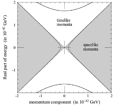
FIG. 7.: Real part of the energy $E$ versus a momentum component for the model parameters (23). The dotted lines correspond to the momentum-space lightcone. The solid and dashed branches are associated with the various roots of the dispersion relation (37). Note the presence of spacelike momenta and superluminal group velocities.

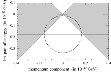
FIG. 8.: Imaginary part of the energy $E$ versus a momentum component for the model parameters (23). The dotted lines represent the momentum-space lightcone. The solid and dashed lines correspond to the respective solid and dashed branches in Fig. 7. For large values of the momentum, the solid and dashed lines lie on top of each other. The region of spacelike momenta is shaded.

Asymptotically, the magnitude of the group velocity $\vec{v}_{\rm g}=\nabla_{\!\vec{p}}\>E(\vec{p})$ equals unity because the conventional Lorentz-symmetric term $(p^{\mu}p_{\mu})^{2}$ dominates the dispersion relation (37) at high energies. However, inspection of the slope of a dashed branch in Fig. 7 reveals the possibility that $|\vec{v}_{\rm g}|>c$ at low energies. For a background that is fixed and fundamentally nondynamical, such superluminal group velocities violate microcausality [32]. But for conventional dynamical backgrounds leading to group velocities exceeding $c$, causality is typically maintained. Examples in ordinary electrodynamics can be readily identified: the occurrence of superluminal $\vec{v}_{\rm g}$ in amplifying media with inverted atomic populations has been verified theoretically and experimentally [43], but causality violations are absent [44]. The underlying Lorentz-covariant dynamics of the our supergravity cosmology leads therefore to the conjecture that causality is maintained in the present context. The apparent superluminal particle propagation would then be an artifact of the approximations employed in the derivation of the dispersion relation (37). A complete investigation of these issues would be interesting but lies well outside the scope of this work.

For completeness, the imaginary part of the energy variable as a function of momentum is plotted in Fig. 8. The momentum-space lightcone is again represented by the dotted line. The shaded region is associated with spacelike 4-momenta. The solid and dashed lines correspond to the solid and dashed branches in Fig. (7). At large 3-momenta, all four branches overlap and ${\rm Im}(E)$ is bounded, which is in agreement with Eq. (43).

VI Summary

This work has considered cosmologies with scalar fields that are motivated in candidate fundamental theories. In such a context, the scalars typically acquire varying expectation values that can be associated with an accelerated expansion of the universe, varying couplings, and Lorentz-violation.

More specifically, we have investigated an $N=4$ supergravity model in four dimensions. In this framework, standard plausible arguments lead to a variation of the axion and the dilaton on cosmological scales. As a result, the propagation of the axion and the dilaton is governed by a Lorentz-violating effective dispersion relation. We expect this feature to be generic in models with scalars varying on cosmological scales.

The axion-dilaton background also affects the expansion of the universe and results in spacetime-dependent electromagnetic couplings. Model parameters exist that lead to a behavior of the scale factor consistent with the observed late-time cosmological expansion. The variation of $\alpha$ implied by this parameter set lies mostly outside experimental constraints. However, the time dependence of $\alpha$ is roughly in the order of magnitude suggested by the Webb data and displays desirable nonlinear features.

A Additional remarks regarding the spectrum of solutions

We begin our considerations with the observation that for all nontrivial physical input values the universe is always expanding in our supergravity cosmology. Suppose this were not the case. Then, at some time $t=t_{0}$, there must be a transition from the presently observed cosmological expansion to a subsequent epoch involving contraction. This implies $\dot{a}(t_{0})=0$ at the time $t_{0}$ by continuity of $\dot{a}(t)$. Then, the first of the Einstein equations (9) yields at $t=t_{0}$

$$m_{A}^{2}A^{2}+m_{B}^{2}B^{2}+{{\dot{A}^{2}+\dot{B}^{2}}\over{2B^{2}}}+2\rho=0\;,$$ (A1)

which can only be satisfied in the trivial situation of an empty universe with zero total energy density or in unphysical cases involving negative matter densities $\rho<0$.

We continue our discussion by considering special choices for the parameters $m_{A}$ and $m_{B}$. The situation $m_{A}=0$ and $m_{B}=0$ has been discussed previously in the literature [16]. Let us therefore focus first on the case $m_{A}\neq 0$ and $m_{B}=0$. With this choice, we find the following analytical solution:

$$a(t) = \sqrt[3\;]{3c_{\rm n}}\;t^{2/3}\;,$$ (A2)

$$A(t) = \pm(m_{A}t)^{-1}\;,$$ (A3)

$$B(t) = \pm(m_{A}t)^{-1}\;.$$ (A4)

Here, the signs in the equations for $A(t)$ and $B(t)$ can be selected independently. The absence of integration constants indicates that more general solutions exist (cf. model P2 below). Note that the cosmological expansion implied by Eqs. (A4) is essentially that of a conventional matter-dominated universe, which always decelerates. The time dependence of the fine-structure parameter is given by

$$\alpha(t)={{1}\over{4\pi}}\;{{4+m_{A}^{4}t^{4}}\over{2m_{A}t+m_{A}^{3}t^{3}}}\;.$$ (A5)

It follows that at late times, $\alpha$ increases linearly with $t$.

Next, we look at the case $m_{A}=0$ and $m_{B}\neq 0$. One can verify that

$$a(t) = \sqrt[3\;]{{\textstyle{{6}\over{5}}}c_{\rm n}}\;t^{2/3}\;,$$ (A6)

$$A(t) = A_{0}+A_{3}t^{-3}\;,$$ (A7)

$$B(t) = \pm\sqrt{2}(m_{B}t)^{-1}\;,$$ (A8)

is an asymptotic $(t\rightarrow\infty)$ solution. The integration constants $A_{0}$ and $A_{3}$ can be chosen freely. This solution also describes a non-accelerated cosmological expansion. For $A_{0}\neq\pm 1$, the late-time behavior of $\alpha(t)$ is given by

$$\alpha(t)={{1}\over{4\sqrt{2}\pi}}\;{{(1-A_{0}^{2})^{2}}\over{1+A_{0}^{2}}}m_{B}t\;.$$ (A9)

In a situation with $A_{0}=\pm 1$, the fine-structure parameter decreases asymptotically as follows:

$$\alpha(t)=(\sqrt{2}\pi m_{B}t)^{-1}\;.$$ (A10)

We also mention that with the choice $A_{3}=0$, Eqs. (A8) become an exact solution. In this case, the time-evolution of the electromagnetic coupling reads

$$\alpha(t)={{1}\over{4\pi}}\;{{4+4(1+A_{0}^{2})m_{B}^{2}t^{2}+(1-A_{0}^{2})^{2}m_{B}^{4}t^{4}}\over{2\sqrt{2}m_{B}t+\sqrt{2}(1+A_{0}^{2})m_{B}^{3}t^{3}}}\;.$$ (A11)

The general situation, in which both $m_{A}$ and $m_{B}$ are nonzero, seems to evade systematic analysis with analytical methods. Numerical investigations reveal the existence of a broad spectrum of qualitatively different solutions. Figure 9 conveys a flavor of the diversity in acceleration behavior of our supergravity cosmology. The second derivative of the scale factor, $\ddot{a}(t)$, is plotted versus the comoving time $t$ for the four parameter sets P1 to P4 given in Table I. The shaded region marks accelerated cosmological expansion. The input values P1 are associated with a cosmology of permanent deceleration, qualitatively analogous to a conventional matter-dominated universe without cosmological constant. The model parameters P2 lead to an initial deceleration period followed by an asymptotic accelerated expansion. This behavior agrees qualitatively with that of the phenomenological model (23). An overall decelerated expansion with a transient period of acceleration results from the input P3. The parameter set P4 implies an initial deceleration, followed by transient periods of acceleration and deceleration before the expansion continues to accelerate.

It is worth emphasizing that some of the solutions we have obtained exhibit the interesting feature of a transient accelerated expansion (cf. model P3). This is a possible fix for the recently discussed problem concerning an eternally accelerated cosmological expansion. Such universes would pose a challenge for string theory, at least in its present formulation, since string asymptotic states are inconsistent with spacetimes that possess event horizons in the future [45].

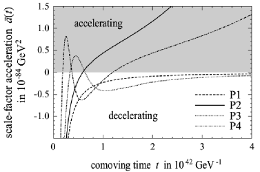
FIG. 9.: Acceleration $\ddot{a}(t)$ of the scale factor versus comoving time $t$ for the various input values given in Table I. The shaded region corresponds to accelerated expansion. The diversity in qualitative behavior is apparent.

TABLE I. Input-parameter sets P1, P2, P3, and P4. Parameter   P1 P2 P3 P4 $m_{A}$ in $10^{-42}\,{\rm GeV}$   0 1.5 0 1 $m_{B}$ in $10^{-42}\,{\rm GeV}$   10 0 100 100 $c_{\rm n}$ in $10^{-84}\,{\rm GeV}^{2}$   2 2 2 2 $a(t_{\rm n})$   1 1 1 1 $A(t_{\rm n})$   1.023 1.023 1.023 1.023 $\dot{A}(t_{\rm n})$ in $10^{-47}\,{\rm GeV}$   47 47 47 -100 $B(t_{\rm n})$    0.022   0.022   0.022   0.022 $\dot{B}(t_{\rm n})$ in $10^{-45}\,{\rm GeV}$   -25 -25 -25 -60 $t_{\rm n}$ in $10^{40}\,{\rm GeV}^{-1}$   56 51 54 51

REFERENCES

- [1] S.J. Perlmutter et al., [Supernova Cosmology Project Collaboration], Astrophys. J. 483, 565 (1997); Nature (London) 391, 51 (1998); A.G. Riess et al., [Supernova Search Team Collaboration], Astron. J. 116, 1009 (1998); P.M. Garnavich et al., Astrophys. J. 509, 74 (1998).
- [2] See, e.g., M.C. Bento and O. Bertolami, Gen. Rel. Grav. 31, 1461 (1999); M.C. Bento, O. Bertolami, and P.T. Silva, Phys. Lett. B 498, 62 (2001), and references therein.
- [3] For early work in the subject, see, e.g., M. Bronstein, Phys. Zeit. Sowjetunion 3, 73 (1993); O. Bertolami, Nuovo Cim. B 93, 36 (1986); Fortsch. Phys. 34, 829 (1986); M. Ozer and M.O. Taha, Nucl. Phys. B 287, 776 (1987); B. Ratra and P.J.E. Peebles, Phys. Rev. D 37, 3406 (1988); Astrophys. J. 325, L17 (1988); C. Wetterich, Nucl. Phys. B 302, 668 (1988).
- [4] R.R. Caldwell, R. Dave, and P.J. Steinhardt, Phys. Rev. Lett. 80, 1582 (1998); P.G. Ferreira and M. Joyce, Phys. Rev. D 58, 023503 (1998); I. Zlatev, L. Wang, and P.J. Steinhardt, Phys. Rev. Lett. 82, 896 (1999); P. Binétruy, Phys. Rev. D 60, 063502 (1999); J.E. Kim, JHEP 9905, 022 (1999); J.P. Uzan, Phys. Rev. D 59, 123510 (1999); T. Chiba, Phys. Rev. D 60, 083508 (1999); L. Amendola, Phys. Rev. D 60, 043501 (1999); O. Bertolami and P.J. Martins, Phys. Rev. D 61, 064007 (2000); N. Banerjee and D. Pavón, Phys. Rev. D 63, 043504 (2001); A.A. Sen, S. Sen, and S. Sethi, Phys. Rev. D 63, 107501 (2001); A. Albrecht and C. Skordis, Phys. Rev. Lett. 84, 2076 (2000).
- [5] A. Masiero, M. Pietroni, and F. Rosati, Phys. Rev. D 61, 023504 (2000); Y. Fujii, Phys. Rev. D 62, 044011 (2000); M.C. Bento, O. Bertolami, and N.C. Santos, Phys. Rev. D 65, 067301 (2002).
- [6] C. Armendáriz-Picón, T. Damour, and V. Mukhanov, Phys. Lett. B 458, 209 (1999); T. Chiba, T. Okabe, and M. Yamaguchi, Phys. Rev. D 62, 023511 (2000); C. Armendáriz-Picón, V. Mukhanov, and P.J. Steinhardt, Phys. Rev. Lett. 85, 4438 (2000).
- [7] A. Kamenshchik, U. Moschella, and V. Pasquier, Phys. Lett. B 511, 265 (2001); M.C. Bento, O. Bertolami, and A.A. Sen, Phys. Rev. D 66, 043507 (2002); N. Bilić, G.B. Tupper, and R.D. Viollier, Phys. Lett. B 535, 17 (2002); J.C. Fabris, S.V.B. Gonçalves, and P.E. de Souza, Gen. Rel. Grav. 34, 53 (2002); M.C. Bento, O. Bertolami, and A.A. Sen, Phys. Rev. D 67, 063003 (2003); astro-ph/0303538.
- [8] J.K. Webb et al., Phys. Rev. Lett. 82, 884 (1999); 87, 091301 (2001); M.T. Murphy, J.K. Webb, V.V. Flambaum, and S.J. Curran, Astrophys. Space Sci. 283, 577 (2003).
- [9] P.A.M. Dirac Nature (London) (London) 139, 323 (1937).
- [10] See, e.g., E. Cremmer and J. Scherk, Nucl. Phys. B 118, 61 (1977); A. Chodos and S. Detweiler, Phys. Rev. D 21, 2167 (1980); W.J. Marciano, Phys. Rev. Lett. 52, 489 (1984); T. Damour and A.M. Polyakov, Nucl. Phys. B 423, 532 (1994), P. Lorén-Aguilar, E. García-Berro, J. Isern, and Y.A. Kubyshin, Class. Quant. Grav. 20, 3885 (2003).
- [11] For recent reviews see, e.g., T. Chiba, gr-qc/0110118; J.P. Uzan, Rev. Mod. Phys. 75, 403 (2003).
- [12] J.D. Bekenstein, Phys. Rev. D 25, 1527 (1982).
- [13] K.A. Olive and M. Pospelov, Phys. Rev. D 65, 085044 (2002).
- [14] C.L. Gardner, astro-ph/0305080.
- [15] L. Anchordoqui and H. Goldberg, Phys. Rev. D, in press [hep-ph/0306084]; E.J. Copeland, N.J. Nunes, and M. Pospelov, hep-ph/0307299; J. Khoury and A. Weltman, astro-ph/0309411; D.F. Mota and J.D. Barrow, astro-ph/0309273.
- [16] V.A. Kostelecký, R. Lehnert, and M.J. Perry, Phys. Rev. D, in press, [astro-ph/0212003].
- [17] V.A. Kostelecký and S. Samuel, Phys. Rev. D 39, 683 (1989); 40, 1886 (1989); Phys. Rev. Lett. 63, 224 (1989); 66, 1811 (1991); V.A. Kostelecký and R. Potting, Nucl. Phys. B 359, 545 (1991); Phys. Lett. B 381, 89 (1996); Phys. Rev. D 63, 046007 (2001); V.A. Kostelecký, M.J. Perry, and R. Potting, Phys. Rev. Lett. 84, 4541 (2000).
- [18] G. Amelino-Camelia et al., Nature (London) 393, 763 (1998).
- [19] D. Sudarsky, L. Urrutia, and H. Vucetich, gr-qc/0211101. Phys. Rev. D 68, 024010 (2003).
- [20] F.R. Klinkhamer, Nucl. Phys. B 578, 277 (2000).
- [21] J. Alfaro, H.A. Morales-Técotl, and L.F. Urrutia, Phys. Rev. Lett. 84, 2318 (2000); Phys. Rev. D 65, 103509 (2002).
- [22] S.M. Carroll et al., Phys. Rev. Lett. 87, 141601 (2001); Z. Guralnik et al., Phys. Lett. B 517, 450 (2001); A. Anisimov et al., Phys. Rev. D 65, 085032 (2002); C.E. Carlson et al., Phys. Lett. B 518, 201 (2001).
- [23] See, e.g., P. de Bernardis et al., [Boomerang Collaboration], Nature (London) 404, 955 (2000); A.E. Lange et al., [Boomerang Collaboration], Phys. Rev. D 63, 042001 (2001); C.L. Bennet et al., [WMAP Collaboration], astro-ph/0302207; D.N. Spergel et al., [WMAP Collaboration], astro-ph/0302209.
- [24] E. Cremmer and B. Julia, Nucl. Phys. B 159, 141 (1979).
- [25] A. Das, M. Fischler, and M. Roček, Phys. Rev. D 16, 3427 (1977).
- [26] S.J. Perlmutter and B.P. Schmidt, astro-ph/0303428.
- [27] T. Damour and F. Dyson, Nucl. Phys. B 480, 37 (1996); Y. Fujii et al., Nucl. Phys. B 573, 377 (2000); K. Olive et al., hep-ph/0205269.
- [28] There exist also parameter choices leading to a variation of that approximately matches observations [16, 29]. In these cases, however, the resulting cosmological expansion is phenomenologically uninteresting.
- [29] R. Lehnert, hep-ph/0308208.
- [30] D. Colladay and V.A. Kostelecký, Phys. Rev. D 55, 6760 (1997).
- [31] V.A. Kostelecký and R. Potting, Phys. Rev. D 51, 3923 (1995); D. Colladay and V.A. Kostelecký, Phys. Rev. D 58, 116002 (1998).
- [32] V.A. Kostelecký and R. Lehnert, Phys. Rev. D 63, 065008 (2001).
- [33] O. Bertolami et al., Phys. Lett. B 395, 178 (1997).
- [34] V.A. Kostelecký and M. Mewes, hep-ph/0308300; hep-ph/0309025.
- [35] For recent experimental progress and theoretical ideas in this subject, see CPT and Lorentz Symmetry II, edited by V.A. Kostelecký (World Scientific, Singapore, 2002).
- [36] S.M. Carroll, G.B. Field, and R. Jackiw, Phys. Rev. D 41, 1231 (1990).
- [37] V.A. Kostelecký and M. Mewes, Phys. Rev. Lett. 87, 251304 (2001); Phys. Rev. D 66, 056005 (2002).
- [38] D. Bear et al., Phys. Rev. Lett. 85, 5038 (2000).
- [39] R. Lehnert, Phys. Rev. D 68, 085003 (2003).
- [40] O. Bertolami and C.S. Carvalho, Phys. Rev. D 61, 103002 (2000); T.J. Konopka and S.A. Major, New J. Phys. 4, 57 (2002); Jacobson et al., astro-ph/0309681.
- [41] In a local comoving inertial frame, the time coordinate agrees to first order with comoving time , so that we can take .
- [42] C. Adam and F.R. Klinkhamer, Nucl. Phys. B 607, 247 (2001).
- [43] R.Y. Chiao, Phys. Rev. A 48, 34 (1993); A.M. Steinberg and R.Y. Chiao, Phys. Rev. A 49, 2071 (1994); E.L. Bolda, J.C. Garrison, and R.Y. Chiao, Phys. Rev. A 49, 2938 (1994).
- [44] See, e.g., G. Diener, Phys. Lett. A 223, 327 (1996); Phys. Lett. A 235, 118 (1997).
- [45] S. Hellerman, N. Kaloper, and L. Susskind, JHEP 0106, 003; W. Fischler, A. Kashani-Poor, R. McNess, and S. Paban, JHEP 0107, 003 (2001); E. Witten, hep-th/0106109.