[astro-ph/0310343] Extinction Properties of Some Complex Dust Grains

1. Introduction

The shape of interstellar and circumstellar grains is still an outstanding issue. The complexity of the electromagnetic scattering problem limits the theoretical modeling of the shapes which can be studied to spheres, infinite cylinders and spheroids. However, the shape of many interstellar grains are expected to be non-spherical and maybe even highly irregular. One way to deal theoretically with irregular particles and clusters of dust grains is to assume that they consist of touching spheres. With such an assumption it is possible to construct many distinctly different morphologies which can then be compared with observations.

The problem of evaluating the extinction efficiency ( $Q_{\rm ext}$ ) is that of solving Maxwell’s equations with appropriate boundary conditions at the cluster surface. For a homogeneous single sphere a solution was formulated by Lorenz (1890) and Mie (1908) and the complete formalism is therefore often referred to as the Lorenz-Mie theory. A complementary solution based on the expansion of scalar potentials was given by Debye (1909). A detailed description of this exact electromagnetic solution can be found in the book by Bohren & Huffman (1983). For a review on exact theories and numerical techniques for computing the scattered electromagnetic field by clusters of particles we refer the reader to the textbook by Mishchenko et al. (2000). For a comprehensive review on the optics of cosmic dust see Voshchinnikov (2002) and Videen & Kocifaj (2002).

To investigate clustering effects we have computed and analyzed the extinction of different polycrystalline graphitic and silicate clusters. We have chosen clusters ranging from small to large, and which are either sparse or compact, to evaluate how the extinction is influenced by the structure. We focus on clusters consisting of 4, 7, 8, 27, 32 and 49 touching polycrystalline spheres with a radius of 10 nm. The extinction of the clusters is calculated using two rigorous methods – GA (Gérardy & Ausloos 1982), and the generalized multi-particle Mie (GMM) solution (Xu 1995; 1997) – and two discrete dipole approximation (DDA) methods – MarCoDES (Markel 1998) and DDSCAT (Draine & Flatau 2000) – to test how well these latter approximations perform when applied to clusters with different morphology. DDSCAT is as such an exact solution if enough dipoles are used in the approximation of the target. It has been used in a wide range of scattering problems concerning clusters of particles including the extinction of interstellar dust grains (e.g. Bazell & Dwek 1990; Wolff et al. 1994; Stognienko et al. 1995; Fogel & Leung 1998; Vaidya et al. 2001). The rigorous solutions are only exact if a high enough number of multi-poles is treated.

2. Structure of the clusters

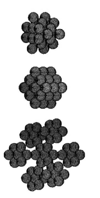
Refer to caption — Figure 1.: Some of the clusters considered in the calculations. From left to right: the prefractal clusters frac7 and frac49; the simple cubic clusters sc8 and sc27; and the face-center-cubic clusters fcc4 and fcc32. The numerical suffixes indicate the number of spheres in the clusters.

We consider three-dimensional clusters of identical touching spherical particles, of radius R, arranged in three different geometric configurations: prefractal (frac), simple cubic (sc), and face-centered cubic (fcc). These structures do not have shapes expected to be found in space, but will provide us with boundary conditions for the problem of calculating the extinction of clusters of grains of different morphologies.

The snowflake prefractal of $n$ ’th–order is recursively constructed starting with the initiator which is just a single sphere. Next, the 1’st–order prefractal, or generator, is built up by pasting together seven copies of the initiator as shown in the top left hand corner frame of Fig. 1. For $n>1$ , pasting together seven copies of the $n-1$ ’th order prefractal according to the generator’s pattern yields the $n$ ’th order prefractal. For example, the bottom left hand corner frame of fig. 1 displays the snowflake prefractal of order 2. As its order increases and goes to infinity, the snowflake prefractal will become the snowflake fractal.

Vicsek (1983) has shown that regardless of their order all the snowflake prefractals have the same dimension, $D=\ln 7/\ln 3=1.77$ , which is exactly the dimension of the snowflake fractal. This value is close to that obtained for random cluster-cluster aggregation models for grain growth (Meakin 1988; Botet and Jullien 1988; Meakin & Jullien 1988; Wurm & Blum 1998).

As a contrast to the prefractal structure, we also consider some compact crystalline structures, namely, face-centered cubic and simple cubic, see e.g. Kittel (1986) for a discussion on crystal structures. All of the clusters we consider are symmetric, see Fig. 1, and consist of spheres with radii $R=10$ nm.

3. Material properties

For our clusters we consider two different materials; graphite and silicates. Graphite can be characterized by two different dielectric functions, $\epsilon_{\perp}$ and $\epsilon_{\parallel}$ , corresponding to the electric-field vector ${\bf E}$ being perpendicular ( $\epsilon_{\perp}$ ) and parallel ( $\epsilon_{\parallel}$ ) to the symmetry axis of the crystal ( $c$ -axis), which is perpendicular to the basal plane. It is far easier to experimentally determine $\epsilon_{\perp}$ than $\epsilon_{\parallel}$ , because graphite cleaves readily along the basal plane and hence reflectivity measurements can be made with normal incident light, in contrast, it is very difficult to prepare suitable optical surfaces parallel to the $c$ -axis. We use the dielectric functions $\epsilon_{\parallel}$ and $\epsilon_{\perp}$ of graphite derived by Draine & Lee (1984) covering the region from the far-IR to the far-UV. For the silicates we use the dielectric function of astronomical silicates in the form given by Weingartner & Draine (2001). The dielectric functions of the two materials are shown in Fig. 2.

As discussed by Draine & Lee (1984) the dielectric constants for graphite are both temperature and size dependent. The graphite data obtained from Bruce Draine (http://www.astro.princeton.edu/ $\sim$ draine/dust/dust.diel.html) are given for particle radius $R=100$ nm. When using the data for other grain sizes it is necessary to correct the data according to Eq. 2 in Draine & Lee (1984)¹¹1Notice that the plasma frequency for $\epsilon_{\perp}$ should be taken from the Errata (Draine & Lee 1987).. The effect of the size corrections on the (average) optical constants $n$ and $k$ are shown in Fig. 3 for different grain sizes. The correction is most significant in the long wavelength range ( $\lambda>50~{}\mu$ m).

In this work we deal with the anisotropy of graphite by assuming that in all our clusters, each individual particle is polycrystalline having a dielectric function $\epsilon_{\rm ave}$ given by the arithmetic average of $\epsilon_{\parallel}$ and $\epsilon_{\perp}$ , namely $\epsilon_{\rm ave}=\frac{1}{3}\epsilon_{\parallel}+\frac{2}{3}\epsilon_{\perp}$ . For a polycrystal the arithmetic average is a realistic model for $\epsilon_{\rm ave}$ , since Avellaneda et al. (1988) have shown that it is an attainable upper bound for its dielectric function. In stellar environments grains are most likely to grow as polycrystalline or even amorphous particles rather than as mono-crystalline (Gail & Sedlmayr 1984; Sedlmayr 1994). In the usual “1/3 $-$ 2/3” approximation each individual particle is treated as a mono-crystalline, where 1/3 of the cluster particles are assumed to have dielectric function $\epsilon_{\parallel}$ and the remaining 2/3 to have dielectric function $\epsilon_{\perp}$ . This approximation has been shown by Draine (1988) and Draine & Malhotra (1993) to have a surprisingly good accuracy for graphite grains with radii $\leq 200$ Å. However, for larger particles assuming polycrystalline particles seems much more viable, see e.g. Rouleau et al. (1997) for a discussion about different ways of obtaining an average dielectric function for graphite.

4. The computational methods

4.1. The rigorous solutions

Multi-particle scattering shows effects both of interaction and interference of scattered waves from the particles which can give rise to distinct features not seen in single-particle scattering.

The two rigorous solutions presented here are generalized Mie theories giving each a complete solution to the multi-sphere light scattering problem. They are both based on the exact solution of Maxwell’s equations for arbitrary cluster geometries, polarization and incidence direction of the exciting light.

GA:

A rigorous and complete solution to the multi-sphere light scattering problem has been given by Gérardy & Ausloos (GA) (1980; 1982; 1983; 1984) as an extension of the Mie-Ruppin theory (Mie 1908; Ruppin 1975). The solution is obtained by expanding the various fields involved in terms of vector spherical harmonics (VSH). Boundary conditions are extended to account for the possible existence of longitudinal plasmons in the spheres. High-order multi-polar electric and magnetic interaction effects are included.

We consider a cluster of $N$ homogeneous spheres of radius $R$ and dielectric function $\epsilon$ , embedded in a matrix of dielectric constant $\epsilon_{M}$ and submitted to a plane polarized time harmonic electromagnetic field. The total scattered field from the cluster is represented as a superposition of individual fields scattered from each sphere. The electromagnetic field impinging on each sphere consist of the external incident wave and the waves scattered by the other spheres. For any sphere, the incident, internal and scattered fields are expressed in VSH centered at the sphere origin. The boundary conditions on its surface are solved by transforming all relevant field expansions into the sphere coordinate system, yielding a system of $2NL(L+2)$ equations whose solution is the $2^{L}$ -polar approximation to the electromagnetic response of the cluster. For a short description of this method see Andersen et al. (2002).

GMM:

A neat analytical far-field solution to the electromagnetic scattering by an aggregate of spheres in a fixed orientation is provided by Xu (1995; 1997; 1998a; 1998b and Xu et al. 1999), and is implemented in the FORTRAN code gmm01f.f (GMM) available at http://www.astro.ufl.edu/ $\sim$ xu. As any other rigorous solution to the multi-particle scattering, his approach considers two cooperative scattering effects: interaction and interference of scattered waves from individual particles (Xu & Khlebtsov 2003). Nevertheless, his treatment of the second effect is novel. When a plane wave is incident upon the particles (scatterers) of a cluster, it has a phase difference determined by the geometrical configuration and spatial orientation of the cluster. Likewise, far away from the scatterers, the waves scattered from them also have well defined phase relations that depend on the scattering direction. These incident and scattered phase differences give rise to far-field interference effects. Xu (1997) includes the incident-wave phase terms in the incident-field expansions centered on each scatterer, and the scattered-wave phase terms in the single-field representation of the total scattered far-field from the whole cluster. This way of treating the interference effects is in practical calculations quite efficient because then the required multipole order of the field expansions will depend only on the size of the individual particles and not on the distance between them, that is, it will not depend on the size of the cluster (Xu & Khlebtsov 2003). This allows in principle the treatment of clusters of arbitrary size; the only limiting factor being the availability of computer memory. In general, an adequate estimate for the field-expansion truncation of all the scatterers in a cluster is given by the Wiscombe’s criterion (Wiscombe 1980) for the field-expansion truncation of a single sphere with size parameter $x$ , $L\approx x+4x^{1/3}+2$ . There are a number of cases, however, where this criterion grossly underestimates the number of multipoles needed in the scattering calculations. This is the case for our clusters of graphitic spheres as it is for the gold nano-bispheres discussed by Xu & Khlebtsov (2003), and the soot bispheres discussed by Mackowski (1994). For example, to get a converged solution to the multi-particle scattering problem at wavelength 1.047 microns for a cluster of 8 graphitic spheres of radii 10 nm, arranged in a simple cubic structure, the actual single-sphere expansion truncation is 44 whereas the Wiscombe’s criterion estimate is just 3. Finally, GMM implements two methods for solving the system of linear equations arising in multi-particle scattering, namely the order of scattering method of Fuller and Kattawar (1988a; 1988b) and the biconjugate gradient method (Gutknecht 1993).

4.2. The discrete dipole approximations

The discrete dipole approximation (DDA) - also known as the coupled dipole approximation - method is one of several discretization methods (e.g. Draine 1988; Hage & Greenberg 1990) for solving scattering problems in the presence of a target with arbitrary geometry. The discretization of the integral form of Maxwell’s equations is usually done by the method of moments (Harrington 1968). Purcell & Pennypacker (1973) were the first to apply this method to astrophysical problems; since then, the DDA method has been improved greatly by Draine (1988), Goodman et al. (1991), Draine & Goodman (1993), Draine & Flatau (2000), Markel (1998), and Draine (2000). The DDA method has gained popularity among scientists due to its clarity in physical principle and the FORTRAN implementation which have been made publicly available by e.g. Draine & Flatau (2000; DDSCAT) and by Markel (Markel 1998; MarCoDES).

Within the framework of the DDA method, when considering the problem of scattering and absorption of linearly polarized light

E_{0}=e_{0}\exp\left(ikr\right)

(1)

of wavelength $\lambda=2\pi/k$ by an isotropic grain, the grain is replaced by a set of discrete elements of volume $V_{i}$ with relative dielectric constant $\epsilon_{i}$ and dipole moments $d_{i}=d\left(r_{i}\right)$ , $i=1,...,N,$ whose coordinates are specified by vectors $r_{i}$ . The equations for the dipole moments can be written using simple considerations based on the concept of the exciting field, which is equal to the sum of the incident wave and the fields of the rest of the dipoles in a given point.

DDSCAT:

In this work we use the Discrete Dipole Approximation Code version 5a10 (DDSCAT; Draine & Flatau 1994; Draine & Flatau 2000), available at
http://www.astro.princeton.edu/ $\sim$ draine/DDSCAT.html. This version contains a new shape option where a target can be defined as the union of the volumes of an arbitrary number of spheres. In DDSCAT the considered grain/cluster is replaced by a cubic array of point dipoles. The cubic array has numerical advantages because the conjugate gradient method can be efficiently applied to solve the matrix equation describing the dipole interactions (Goodman et al. 1991).

There are three criteria for the validity of DDSCAT:
(1) The wave phase shift $\rho=|m|ka$ over the distance $a$ between neighboring dipoles should be less than 1 for calculations of total cross sections and less than 0.5 for phase function calculations. Here, $m=\sqrt{\epsilon}=n+ik$ is the complex refractive index of the target material
(2) $a$ must be small enough to describe the object shape satisfactorily.
(3) The refractive index $m$ must fulfill $|m|<2$ .

For materials with large refractive indexes ( $|m|>2$ ), Draine & Goodman (1993) have shown that especially the absorption is overestimated by DDA. As illustrated in Fig. 2, graphite has a high refractive index throughout most of the range $0.03-100~{}\mu$ m, showing that for graphite the region of applicability of DDSCAT is rather small, in fact, the criterion $|m|<2$ is only fulfilled for wavelengths shorter than $\lambda=0.072~{}\mu$ m ( $m=0.58+i1.42$ ); see the inset in the left frame of Fig. 2. However, relaxing the criterion a little, to account for the variability of $m$ in the region below $1.0~{}\mu$ m, the upper limit can be pushed up to $\lambda=0.216~{}\mu$ m ( $m=0.66+i1.35$ ).

MarCoDES:

Another efficient code based on DDA is the Markel Coupled Dipole Equation Solver (MarCoDES; Markel 1998) available at
http://atol.ucsd.edu/ $\sim$ pflatau/scatlib/. This code is designed to approximate the spherical particles in an arbitrary cluster with $point$ dipoles (this corresponds to $N=1$ in DDSCAT). The program is in principle applicable to clusters of arbitrary geometry consisting of small spherical particles, but it is most efficient computationally for sparse clusters (i.e. when the volume fraction is very low) with significant number of particles $(\approx 10^{3}-10^{4})$ . Unlike DDSCAT, the program does not use the Fast Fourier Transformation (FFT) because this might significantly decrease its computational performance on clusters with a low volume filling fraction. When the volume filling fraction is close to unity, algorithms utilizing FFT will be much faster.

The dimensionality of the coordinates of particles in MarCoDES require a special consideration. By replacing real particles by point dipoles located at their centers the strength of their interaction is significantly underestimated. In order to correct the interaction strength, the author of MarCoDES introduces geometrical intersection of particles. All coordinates are defined in terms of the distance between neighboring dipoles $a$ , which is given by $a=\left(4\pi/3\right)^{1/3}R$ . So, for example, if two particles have radii 10 nm, then the distance between the dipoles is 16.12 nm. This suggested phenomenological procedure allows MarCoDES to be more accurate than the usual single dipole approximation since the intersection produces some analogy of including higher multi-pole interactions between particles. The fact that the program only uses a single dipole for each particle in the cluster has significant benefits in computation efficiency when compared to other multi-polar approaches such as GA, GMM or DDSCAT.

The version of MarCoDES tested here cannot calculate a face-centered cubic structure of touching particles because in this case the lattice cells representing neighboring particles will touch only at the corners, giving as a consequence the spectrum corresponding to non-touching particles.

4.3. Accuracy of the different methods

Within the GA method the extinction of a cluster is calculated in the $2^{L}$ -polar approximation. In general, the smallest L needed for the convergence of the extinction differs for different regions of the optical spectrum; for graphite in particular, for a chosen fixed accuracy, the longer the wavelength, the higher the polar orders that are required in the calculations. This happens because the magnitude of the refractive index of graphite increases with wavelength up to about $80.0~{}\mu$ m, where it reaches a plateau. Generally, the extinction of graphitic clusters needs to be calculated to a higher polar order than that of the silicate clusters to ensure convergence. In the UV-visible range, by accepting an accuracy of 5% in the computation of the extinction, we can use L = 5 for open graphitic clusters and L = 7 for compact graphitic ones; we expect this to hold for clusters of up to a few tens of particles. In Table 1, the cut-off polar order L used in the calculation of the extinction of all the clusters can be found. Full convergence was only achieved for the small clusters in the UV-vis range; for the larger clusters, L indicates the maximum polar order obtained with our available computer resources.

Table 1.: The clusters presented in this paper have three different geometries (see Fig. 1): prefractal (frac; D

=1.77

), face-center cubic (fcc) and simple cubic (sc). L designates the polar order achieved with the GA method.

Cluster Structure	frac	frac	fcc	fcc	fcc	sc	sc
# particles	7	49	4	32	49	8	27
polar order L	11	6	11	6	6	11	7
Designation	frac7	frac49	fcc4	fcc32	fcc49	sc8	sc27

The theory behind GMM is in many ways similar to that behind GA, differing from it in its use of an asymptotic form of the vector translational addition theorem in the calculation of the total scattered wave in the far field, which avoids the severe numerical problems encountered by GA when computing the latter for clusters of a large number of particles. As said earlier, GMM uses either the order of scattering method or the biconjugate gradient method in solving the multi-particle scattering problem. Furthermore, when the former method fails in finding a solution, GMM switches to the latter method, thus providing an answer in the majority of cases, although it may have to use very high polar orders to achieve a desired accuracy. For example, to achieve an accuracy of four significant figures in the extinction of the two small clusters frac7 and sc8, GMM needs to use polar orders as high as L=44 for wavelengths around $1.0~{}\mu$ m. GA, on the other hand, proceeds one polar order at a time, and when it does not converge, it is not possible to establish the accuracy of the solution.

Xing & Hanner (1997) find that the typical number of dipoles needed with DDSCAT to obtain a ”reliable” computational result, can be determined by calculating the minimum number of dipoles needed per particle. When a particle of radius $R$ is represented by a 3-dimensional array of $N$ dipoles, its volume is $Na^{3}$ , which must be equal to $4\pi R^{3}/3$ , hence

N=\frac{4\pi}{3}\left(\frac{R}{a}\right)^{3}=\frac{4\pi}{3}\left(\frac{2\pi R|m|}{\rho\lambda}\right)^{3}\approx 1039\left(\frac{R|m|}{\rho\lambda}\right)^{3}

(2)

since $a$ is related to the wave phase shift $\rho$ by $a=\rho/(|m|k)$ (Draine & Flatau 2000). For instance, for $\lambda\mathrel{\hbox{\hbox to0.0pt{\hbox{\lower 4.0pt\hbox{$\sim$}}\hss}\hbox{$<$}}}0.2~{}\mu$ m, around 30 dipoles are needed for each of our graphitic spheres and for $\lambda\mathrel{\hbox{\hbox to0.0pt{\hbox{\lower 4.0pt\hbox{$\sim$}}\hss}\hbox{$>$}}}0.2~{}\mu$ m just one dipole seem to be enough, indicating that MarCoDES should be comparable with DDSCAT for wavelengths $\lambda\mathrel{\hbox{\hbox to0.0pt{\hbox{\lower 4.0pt\hbox{$\sim$}}\hss}\hbox{$>$}}}0.2~{}\mu$ m.

As illustrated in Fig. 4, for graphitic clusters increasing the number of dipoles used in the DDSCAT calculation does lead to a solution which is slightly closer to the exact result. However, for the frac7 cluster doubling the number of dipoles²²2The two calculations used $36\times 36\times 36$ = 46656 dipoles of which 6265 dipoles represented the cluster (895 dipoles per particle) and $48\times 48\times 48$ = 110592 dipoles of which 14721 dipoles represented the cluster (2103 per particle). only leads to a very slight improvement of the solution. For example, the solution using the lower number of dipoles is about 5% off the exact solution around $\lambda=0.24~{}\mu$ m. Doubling the number of dipoles doubles the computation time while the solution is only improved by less than 1%. According to Eq. (2) we are using more than an adequate number of dipoles for both solutions indicating that a ”reliable” result in the Xing & Hanner (1987) terminology is less accurate than 5%.

As seen from Fig. 5 increasing the number of dipoles used in DDSCAT is not always a guarantee for getting a result which is closer to the exact solution. In the figure two different calculations of the frac49 cluster composed of graphitic spheres are shown. The number of dipoles³³3The two calculations used $40\times 40\times 40$ = 64000 dipoles and $36\times 36\times 36$ = 46656 dipoles. This resulted in 2223 dipoles and 1323 dipoles in the target and $\sim 45$ and $\sim 27$ dipoles per particle, respectively. is almost doubled between the two calculations. A comparison with the GA calculations taken to polar order L=6, shows that almost doubling the number of dipoles improves the result of the DDSCAT calculations by 10 % around $\lambda=0.24~{}\mu$ m. The GA solution is exact in the short wavelength range ( $<0.3~{}\mu$ m) and coincides completely with a calculation of GMM taken to L = 19. At longer wavelengths the GA solution is not fully converged but we expect it to be in the vicinity of the exact solution. The DDSCAT calculations show peculiar behavior at longer wavelengths since the solution using the lower number of dipoles comes much closer to the GA solution than the solution using 30% more dipoles. This indicates that the lower number of dipoles gives a better accuracy for longer wavelengths ( $\lambda>0.3~{}\mu$ m) while the higher number of dipoles gives a better accuracy for shorter wavelengths. In the case of a discrete dipole array, the dipoles in the interior will be effectively shielded, while the dipoles located on the target surface are not fully shielded and, as a result, absorb energy from the external field at an excessive rate. In principle the excess absorption which is introduced by having a large fraction of the dipoles at the surface of the particle should be minimized when introducing more dipoles, but Fig. 5 indicates that it is not necessarily a linear effect. It should be emphasized, however, that the refractive index of the graphitic material have $|m|>2$ at $\lambda>0.3~{}\mu$ m (see Fig. 2) which means that the DDSCAT calculations are outside the range recommended by Draine & Goodman (1993) for its use, so an overestimate of the absorption should be expected. Despite this, increasing the number of dipoles should still lead to an improved solution which is in contrast to what we find. This leaves open the question of ”how many dipoles are enough to assure a certain accuracy in a DDSCAT computation”. We therefore strongly recommend that this question gets investigated in much more detail in the future.

5. Results

To set up a comparison baseline, we computed the extinction of single graphitic and silicate spheres, both of radius 10 nm, using the two rigorous solutions (GA and GMM) and the two DDA codes (DDSCAT and MarCoDES). Since for a single sphere both the GA and GMM theories reduce to the Mie theory, the GA results are exactly the same as those of GMM and equal to the Mie solution, regardless of the sphere’s material. The two DDA codes, however, give results that differ markedly for both graphite and silicate. For graphite, DDSCAT and the Mie solution coincide up to $\lambda\mathrel{\hbox{\hbox to0.0pt{\hbox{\lower 4.0pt\hbox{$\sim$}}\hss}\hbox{$<$}}}1.0~{}\mu$ m, where from DDSCAT starts to diverge slowly from the Mie solution. In contrast, MarCoDES differs from the Mie solution in the region $\lambda\mathrel{\hbox{\hbox to0.0pt{\hbox{\lower 4.0pt\hbox{$\sim$}}\hss}\hbox{$<$}}}0.6~{}\mu$ m. This indicates that for graphite DDSCAT might be the better choice of code for wavelengths $\lambda\mathrel{\hbox{\hbox to0.0pt{\hbox{\lower 4.0pt\hbox{$\sim$}}\hss}\hbox{$<$}}}1.0~{}\mu$ m while MarCoDES is the better choice of code for longer wavelengths. For the silicate, DDSCAT coincides with the Mie solution in the whole wavelength range that we studied ( $0.03-100~{}\mu$ m) while MarCoDES again differs from the Mie solution in the region $\lambda\mathrel{\hbox{\hbox to0.0pt{\hbox{\lower 4.0pt\hbox{$\sim$}}\hss}\hbox{$<$}}}0.6~{}\mu$ m.

Next we study the effect of clustering in the computation of the extinction of graphitic and silicate clusters. As for single spheres, graphitic clusters allow us to better understand the nuances of the different computational methods. For the frac7 cluster (Fig. 6) and the sc8 cluster (Fig. 7) the GMM and GA solution completely agree up to $\lambda\mathrel{\hbox{\hbox to0.0pt{\hbox{\lower 4.0pt\hbox{$\sim$}}\hss}\hbox{$<$}}}2.0~{}\mu$ m showing that the GA solution is indeed converged within the UV-vis region of the spectrum for these clusters. At wavelengths $\lambda\geq 2.0~{}\mu$ m the GA is not fully converged as can be seen from the fact that it underestimates the extinction for both clusters at longer wavelengths. DDSCAT agrees within 5% with the exact solution up to $\lambda\mathrel{\hbox{\hbox to0.0pt{\hbox{\lower 4.0pt\hbox{$\sim$}}\hss}\hbox{$<$}}}1.0~{}\mu$ m at longer wavelengths it underestimates the extinction but only slightly more than the not fully converged GA solution. MarCoDES is 5% off compared to GMM at $\lambda=0.24~{}\mu$ m for the graphitic frac7 cluster and 10% off for the graphitic sc8 cluster at the same wavelength. At wavelengths shortward and longward of $\lambda=0.24~{}\mu$ m MarCoDES significantly underestimates the extinction. For the graphitic frac7 cluster (Fig. 6) MarCoDES performs better than for the sc8 cluster (Fig. 7). According to Markel et al. (2000), the performance of MarCoDES can be improved by altering the intersection parameter which determines if the particles touch or overlap, but we have not investigated that here. Nevertheless, the fact that MarCoDES gives higher extinction than GMM in some cases and lower in others, suggests that the determination of the rather arbitrary optimal intersection parameter is a very complex problem indeed.

For the silicate frac7 cluster (Fig. 7) both the GA, DDSCAT and MarCoDES coincides completely with the exact solution for $\lambda\mathrel{\hbox{\hbox to0.0pt{\hbox{\lower 4.0pt\hbox{$\sim$}}\hss}\hbox{$<$}}}11~{}\mu$ m. At longer wavelengths the GA and DDSCAT solution coincide but overestimate the extinction by about 5% while MarCoDES understimates the extinction at long wavelenghts for the frac7 cluster. For the sc8 silicate cluster (Fig. 8) DDSCAT and GA coincide with the exact solution while MarCoDES underestimates the extinction at $\lambda\mathrel{\hbox{\hbox to0.0pt{\hbox{\lower 4.0pt\hbox{$\sim$}}\hss}\hbox{$<$}}}5~{}\mu$ m and $\lambda\mathrel{\hbox{\hbox to0.0pt{\hbox{\lower 4.0pt\hbox{$\sim$}}\hss}\hbox{$>$}}}10~{}\mu$ m. This suggests that the GA solution is fully converged for the silicate frac7 cluster within the whole wavelength region considered and for the silicate sc8 cluster for $\lambda\mathrel{\hbox{\hbox to0.0pt{\hbox{\lower 4.0pt\hbox{$\sim$}}\hss}\hbox{$<$}}}11~{}\mu$ m. For the silicate clusters the same number of dipoles were used as for the graphitic clusters in the DDSCAT calculations. DDSCAT deviates less than 5% from the exact solution for both of the silicate clusters showing that it performs much better for materials with smaller refractive indices’s than graphite.

Computation time

All of them, GA, GMM and DDSCAT required fairly large amounts of computer time; we point out, however, that all calculations were done on single processor machines (typically with 800 MHz and 256 MB memory) and took at most a few days. The computation time is determined by the accuracy required, and even for a reasonable accuracy it is necessary to use a very fine discretization - i.e. a lot of dipoles for the DDA and high multi-pole orders for the GA and GMM. This leads to a large number of linear equations which needs to be solved for the determination of the scattered electromagnetic field since the scattering matrix is obtained by averaging the scattering matrices over a large number of individual particles. Generally the computation time for a graphitic cluster was 3 times higher than that for the equivalent silicate cluster because of the much higher refractive index of graphite. MarCoDES is by far the fastest of all the methods but its accuracy is sometimes low, especially for compact clusters.

Regarding documentation, DDSCAT, MarCoDES and GMM have well documented user guides which make these programs fairly user friendly. For the GMM code, however, we needed some clarifying correspondence with its author. A new version of DDSCAT is now released (DDSCAT 6.0) which among other things have MPI capability for parallel computations of different target orientations (at a single wavelength); this should be very useful for calculations of averages over orientations (B.T. Draine pers. com.). GMM and MarCoDES are also continuously being improved by their authors.

6. Compact clusters vs. prefractal clusters

We now compare the extinction calculated with the different methods for prefractals and compact clusters.

In Fig. 8, the GA calculation for frac49 is compared to that of fcc32 and sc27 around the 2200 Å absorption feature. Here the conclusion would be (1) the prefractal cluster has a shift in peak position and (2) the extinction of the prefractal clusters are of the same order of magnitude as the compact clusters. At long wavelengths all the considered cluster display an extinction of the same order of magnitude.

Fig. 9 shows the DDA calculations for the compact sc27 cluster and the sparse frac49 cluster. A shift in peak position between the prefractal and the compact cluster is observed around the 2200 Å peak. DDSCAT tends to indicate that the prefractal clusters have a somewhat enhanced extinction around the 2200 Å peak. At long wavelengths both codes show slightly higher extinction for the compact sc27 cluster than for the frac49 cluster.

For the silicate clusters MarCoDES would lead to the conclusion that the prefractal clusters have lower extinction at shorter wavelengths ( $\lambda<1~{}\mu$ m) than the considered compact clusters while with DDSCAT one would conclude that the extinction was of the same order of magnitude for the whole wavelength range in accordance with the GA result.

The GA calculations therefore suggest that the extinction of prefractal and small compact clusters are on the same order of magnitude making it difficult to distinguish the different cluster morphology by observations. With the two DDA codes one might just as well reach the opposite (erroneous) conclusion.

7. Conclusions

We have performed extinction calculations for clusters consisting of polycrystalline graphitic and silicate spheres in the wavelength range $0.1$ to $100~{}\mu$ m. For the computations we have used the rigorous multi-polar theory of Gérardy & Ausloos (1982; GA), the rigorous generalized multi-particle Mie-solution by Xu (1995; GMM); the discrete dipole approximation using one dipole per particle by Markel (1998; MarCoDES) and the discrete dipole approximation using multi dipoles by Draine & Flatau (2000; DDSCAT).

We have compared the extinction of open prefractal clusters and compact clusters. The prefractal and small compact clusters display an extinction of the same order of magnitude as when computed with the exact methods (GA and GMM). At shorter wavelengths around the 2200 Å feature the graphitic prefractal clusters seem to have a stable peak position.

Overall, DDSCAT performs better than MarCoDES for all of the clusters. With DDSCAT, however, there is the unresolved question of how-many-dipoles are needed to ensure a fairly accurate result, this number seems to follow a non-linear pattern so a more accurate result cannot always be expected by doubling the number of dipoles (see Fig. 5). MarCoDES is computationally much faster than the DDSCAT, GMM or GA method. The GMM computations were sufficiently fast so that convergence was reached over the whole studied wavelength range. On the other hand, our available GA program was slower and we could obtain converged results only in the UV-visible wavelength range. Which of the four approaches is best to use for calculating the extinction of cluster particles will depend on the type of problem one wants to address and the accuracy needed.

Acknowledgments.

We would like to thank B.T. Draine, V.A. Markel and Y-L. Xu for making their codes available as shareware. J.S. acknowledges very helpful correspondence with Y-L. Xu regarding the use of GMM.

References

Andersen, A., Sotelo, J., Pustovit, V. & Niklasson, G. 2002, A&A 386, 296

Avellaneda, M., Cherkaev, A.M., Lurie, K.A. & Milton, G.W. 1988, J. Appl. Phys. 63, 4989

Bazell, D. & Dwek, E. 1990, ApJ 360, 262

Bohren, C.F. & Huffman, D.R. 1983, Absorption and Scattering of Light by Small Particles (John Wiley & Sons, New York)

Botet, R. & Jullien, R. 1988, Ann. Phys. (France) 13, 153

Debye, P. 1909, Ann. Phys. 30, 57

Draine, B.T. 1988, ApJ 333, 848

Draine, B.T. & Flatau, P.J. 1994, J. Opt. Soc . Am. A 11, 1491

Draine, B.T. & Flatau, P.J. 2000, User guide for the Discrete Dipole Approximation Code DDSCAT (Version 5a10), http://xxx.lanl.gov/abs/astro-ph/0008151v3

Draine, B.T. & Goodman, J.J. 1993, ApJ 405, 685

Draine, B.T. & Lee, H.M. 1984, ApJ 285, 89

Draine, B.T. & Lee, H.M. 1987, ApJ 318, 485

Draine, B.T. & Malhotra, S.K. 1993, ApJ 325, 864

Draine, B.T. 2000, in Light Scattering by Nonspherical Particles: Theory, Measurements, and Applications, ed. M.I. Mishchenko, J.W. Hovenier & L.D. Travis (Academic Press, New York), 131

Fogel M.E. & Leung C.M., 1998, ApJ 501, 175

Fuller K.A. & Kattawar G.W. 1988a, Opt. Lett. 13, 90

Fuller K.A. & Kattawar G.W. 1988b, Opt. Lett. 13, 1063

Gail H.-P. & Sedlmayr E., 1984, A&A 132, 163

Gérardy, J.M. & Ausloos, M. 1980, Phys. Rev. B 22, 4950

Gérardy, J.M. & Ausloos, M. 1982, Phys. Rev. B 25, 4204

Gérardy, J.M. & Ausloos, M. 1983, Phys. Rev. B 27, 6446

Gérardy, J.M. & Ausloos, M. 1984, Phys. Rev. B 30, 2167

Goodman, J.J., Draine, B.T. & Flatau, P.J. 1991, Opt. Lett. 16, 1198

Gutknecht M.H. 1993, SIAM J. Sci. Comput. 14, 1020

Hage, J.I. & Greenberg, J.M. 1990, ApJ 361, 251

Harrington, R.F. 1968, Field Computation by Moment Methods, (Macmillan, New York)

Kittel, C. 1986, Introduction to Solid State Physics, (Wiley, New York), 11

Lorenz, L. 1890, Vidensk. Selsk. Skr. T. VI(6), (Bianco Lunos Kgl. Hof-Bogtrykkeri, Copenhagen), 1

Mandelbrot, B.B. 1983, The Fractal Geometry of Nature (Freeman, San Francisco)

Markel, V.A. 1998, User guide for MarCoDES - Markel’s Coupled Dipole Equation Solvers, http://atol.ucsd.edu/ $\sim$ pflatau/scatlib/

Markel, V.A., Shalaev, V.M. & George, T.F. 2000, in Optics of Nanostructured Materials, eds. V.A. Markel & T.F. George (Wiley, New York), 355

Mackowski, D.W. 1994, J. Opt. Soc. Am. A 11, 2851

Meakin, P. 1988, Ann. Rev. Phys. Chem. 39, 237

Meakin, P. & Jullien, R. 1988, J. Chem. Phys. 89, 246

Mie, G. 1908, Ann. Phys. Leipz. 25, 377

Mishchenko, M.I., Hovenier, J.W. & Travis, L.D. 2000, Light Scattering by Nonspherical Particles: Theory, Measurements and Applications, (Academic Press, New York)

Purcell, E.M. & Pennypacker, C.R. 1973, ApJ 186, 705

Rouleau, F., Henning, Th. & Stognienko, R. 1997, A&A 322, 633

Ruppin, R. 1975, Phys. Rev. B 11, 2871

Sedlmayr, E. 1994, in Molecules in the Stellar Environment, LNP 428, ed. U.G. Jørgensen (Springer, Berlin), 163

Stognienko R., Henning Th. & Ossenkopf V., 1995, A&A 296, 797

Xing, Z. & Hanner M.S. 1997, A&A 324, 805

Xu, Y-L. 1995, Appl. Opt. 34, 4573

Xu, Y-L. 1997, Appl. Opt. 36, 9496

Xu, Y-L. 1998a, Appl. Opt. 37, 6494

Xu, Y-L. 1998b, Phys. Lett. A 249, 30

Xu, Y-L., Gustafson, B.Å.S., Giovane F., Blum J. & Tehranian S. 1999, Phys. Rev. E 60, 2347

Xu, Y-L. & Khlebtsov N.G. 2003, JQSRT 79-80, 1121

Vaidya, D.B., Gupta, R., Dobbie, J.S. & Chylek, P. 2001, A&A 375, 584

Vicsek G., 1983, J. Phys. A 16, L647

Videen G. & Kocifaj M., 2002, Optics of Cosmis Dust, Nato Science Series: II: Mathematics, Physics and Chemistry volume 79

Voshchinnikov, N.V. 2002, Astroph. & Space Sci. Rev. 12, 1

Weingartner, J.C. & Draine, B.T. 2001, ApJ 548, 296

Wiscombe W.J. 1980, J. Appl. Opt. 19, 1505

Wolff M.J., Clayton G.C., Martin P.G. & Schulte-Ladbeck R.E., 1994, ApJ 423, 412

Wurm, G. & Blum, J. 1998, Icarus 132, 125

Extinction Properties of Some Complex Dust Grains

Abstract