The DEEP Groth Strip Survey XII: The Metallicity of Field Galaxies at $0.26<z<0.82$ and the Evolution of the Luminosity-Metallicity Relation

Abstract

Using spectroscopic data from the Deep Extragalactic Evolutionary Probe (DEEP) Groth Strip survey (DGSS), we analyze the gas-phase oxygen abundances in the warm ionized medium for 64 emission-line field galaxies in the redshift range $0.26<z<0.82$. These galaxies comprise a small subset selected from among 693 objects in the DGSS. They are chosen for chemical analysis by virtue of having the strongest emission lines. Oxygen abundances relative to hydrogen range between $8.4<12+log(O/H)<9.0$ with typical internal plus systematic measurement uncertainties of 0.17 dex. The 64 DGSS galaxies collectively exhibit an increase in metallicity with B-band luminosity, i.e., an L-Z relation like that seen among local galaxies. Using the DGSS sample and local galaxy samples for comparison, we searched for a “second parameter” which might explain some of the dispersion seen in the L-Z relation. Parameters such as galaxy color, emission line equivalent width, and effective radius were explored but found to be uncorrelated with residuals from the the mean L-Z relation.

Subsets of DGSS galaxies binned by redshift also exhibit L-Z correlations with slopes and zero-points that evolve smoothly with redshift. DGSS galaxies in the highest redshift bin ($z=0.6-0.82$) are brighter, on average, by $\sim 1$ mag at fixed metallicity compared to the lowest DGSS redshift bin ($z=0.26-0.40$) and brighter by up to $\sim 2.4$ mag compared to local ($z<0.1$) emission-line field galaxies. Alternatively, DGSS galaxies in the highest redshift bin ($z=0.6-0.82$) are, on average, 40% (0.15 dex) more metal-poor at fixed luminosity compared to local ($z<0.1$) emission-line field galaxies. For $0.6<z<0.8$ galaxies, the offset from the local L-Z relation is greatest for objects at the low-luminosity ($M_{B}>-19$) end of the sample and vanishingly small for objects at the high-luminosity end of the sample ($M_{B}\sim-22$). We compare these data to simple single-zone exponential-infall Pégase2 models which follow the chemical and luminous evolution of galaxies from formation to $z=0$. A narrow range of model parameters can qualitatively produce the slope of the L-Z relation and the observed evolution of slope and zero-point with redshift when at least two of the following are true: 1) low-mass galaxies have lower effective chemical yields than massive galaxies, 2) low-mass galaxies assemble on longer timescales than massive galaxies, 3) low-mass galaxies began the assembly process at a later epoch than massive galaxies. The single-zone models do a reasonable job of reproducing the observed evolution for the low-luminosity galaxies ($M_{B}\sim-19$) in our sample, but fail to predict the relative lack of evolution in the L-Z plane observed for the most luminous galaxies ($M_{B}\sim-22$). More realistic multi-zone models will be required to explain the chemo-luminous evolution of large galaxies.

1 Metallicity as a Measure of Galaxy Evolution

Many recent research programs in galaxy evolution trace changes in correlations between fundamental galaxy properties as a function of cosmic epoch. One such approach compares the number density and luminosity function of galaxies at earlier times (Lilly et al. 1995; Bershady et al. 1997; Sawicki, Lin, & Yee 1997; Lin et al. 1999) to the luminosity function in the nearby universe (Zucca et al. 1997; Marzke et al. 1998; Norberg et al. 2002). Evidence suggests an increase in the number density of small, blue galaxies at earlier times with only a small amount of passive fading among the more luminous, redder galaxies. Other investigations compare the relation between rotation velocity and luminosity (T-F relation; Tully & Fisher 1977) locally with that observed in more distant disk galaxies (e.g., Forbes et al. 1995; Vogt et al. 1996, 1997; Simard & Pritchet 1998). Most results indicate that galaxies of a given rotational amplitude appear 0.2-1.0 mag brighter at $z\sim 1$, although Bershady et al. (1998) argue that the variation is significant for only the bluest galaxies, and Kannappan, Fabricant & Franx (2002) show that Tully-Fisher residuals are strongly correlated with galaxy color. Simard et al. (1999) find no evidence for evolution of the size-magnitude relation among 190 field galaxies out to $z=1.1$ in the Groth Strip (Groth 1994). They show that selection effects favor high surface brightness galaxies in existing surveys. These biases may mimic the appearance of luminosity evolution and/or surface brightness evolution reported in many studies (Schade et al. 1996a, 1996b; Roche et al. 1998; Lilly et al. 1998). Yet another line of investigation compares the Fundamental Plane correlations for early-type galaxies as a function of epoch. Recent results suggest a decrease in the mean mass-to-light ratio with lookback time for elliptical galaxies (van Dokkum & Franx 1996; Kelson et al. 1997). In Paper X of this series, Im et al. (2001) found a brightening of 1-2 mag for early-type $L^{*}$ galaxies out to $z\sim 1$, and in Paper IX of this series, Gebhardt et al. find an increase in the surface brightness by a similar amount.

In this paper we explore the evolution of the correlation between metallicity, $Z$, and total luminosity, i.e., the luminosity-metallicity (L-Z) relation to which nearly all types of local galaxies conform. In early-type systems, absorption line indices provide a measure of the mean stellar iron or magnesium abundances (Faber 1973; Brodie & Huchra 1991; Trager 1999) while in spiral (Zaritsky, Kennicutt, & Huchra 1994) and dwarf systems (Lequeux et al. 1979; French 1980; Skillman, Kennicutt, & Hodge 1989; Richer & McCall 1995) the H II region oxygen abundance relative to hydrogen is the basis of the metallicity measurement. The luminosity-metallicity relation (L-Z) can be used as a sensitive probe and consistency check of galaxy evolution. The metallicity of a galaxy can only increase monotonically with time (unless large-scale infall of primordial gas is invoked), while the luminosity may increase or decrease depending on the instantaneous star formation rate. Metallicity is less sensitive to variations due to transient star formation events in a galaxy’s history. Most models and observations of galaxies at earlier epochs predict higher star formation rates and a larger fraction of blue, star-forming galaxies in the past (e.g., Madau et al. 1996; Lilly et al. 1996; Somerville & Primack 1999). Thus, a high or intermediate-redshift galaxy sample ought to be systematically displaced from the local sample in the luminosity-metallicity plane if individual galaxies participate in these cosmic evolution processes. However, if local effects such as the gravitational potential and “feedback” from winds and supernovae regulate the star formation and chemical enrichment process, then the L-Z relation might be independent of cosmic epoch. Semi-analytic models of Somerville & Primack (1999), for example, show very little evolution of the L-Z relation with redshift. One goal of this paper is to provide data capable of testing these alternative hypotheses.

At high redshift, absorption line surveys have been tracing the chemical evolution of the Lyman-alpha forest and damped Lyman-alpha systems for more than a decade (Bergeron & Stasińska 1986; Sargent et al. 1988; Steidel 1990; Pettini et al. 1997; Lu, Sargent, & Barlow 1997; Prochaska & Wolf 1999), while several studies have recently begun to trace the cosmic chemical evolution of individual galaxies with known morphological and photometric properties. Kobulnicky & Zaritsky (1999) measured H II region oxygen and nitrogen abundances for a sample of 14 compact star-forming galaxies with kinematically narrow emission lines in the range $z=0.1-0.5$. Their sample was found to conform to the local L-Z relation, within observational uncertainties. Carollo & Lilly (2001) studied 13 star-forming galaxies at $0.5<z<1$ from the Canada-France Redshift Survey (CFRS; Lilly et al. 1995) and found no significant evidence for evolution in the L-Z relationship out to $z=1$. However, at larger redshifts of $z>2$, both Kobulnicky & Koo (2000) and Pettini et al. (2001) found that Lyman break galaxies with metallicities between $0.1~{}Z_{\odot}<Z<0.8~{}Z_{\odot}$ are 2-4 magnitudes more luminous than local galaxies of similar metallicity. This deviation from the local L-Z relation demonstrates that the luminosity-to-metal ratio varies throughout a galaxy’s lifetime and is a potentially powerful diagnostic of its evolutionary state.

The DEEP (Deep Extragalactic Evolutionary Probe; Vogt et al. 2003; Paper I) team has been assembling Keck spectroscopic data on galaxies in the Groth Strip survey (Groth 1994) in order to study the evolution of field galaxies. Previous papers in this series include a study of the evolution of the Fundamental Plane (FP) of early-type galaxies (Paper IX; Gebhardt et al. 2003), the evolution of the luminosity function of E/S0 galaxies (Paper X; Im et al. 2001), and the structural parameters of Groth Strip galaxies (Simard et al. 2002; Paper II). In this paper, we explore the chemical properties of 64 star-forming emission-line field galaxies observed as part of the DEEP Groth Strip Survey (DGSS). We measure the interstellar medium oxygen abundances using the the ratio of strong [O II], [O III], and H$\beta$ emission line equivalent widths (e.g., Pagel et al. 1979 as extended by Kobulnicky & Phillips 2003; hereafter KP03). We analyze the degree of metal enrichment as a function of redshift, luminosity, and other fundamental parameters. Throughout, we adopt a cosmology with $H_{0}$=70  km s^-1 Mpc^-1, $\Omega_{m}=0.3$, and $\Omega_{\Lambda}=0.7$.

1.1 Local Comparison Galaxy Samples

In order to establish whether DGSS galaxies systematically differ from nearby galaxies in their chemical or luminous properties, we require a suitable sample of local galaxies for comparison. For a comparable sample of local star-forming galaxies, we compiled three sets of emission-line galaxy spectra from the literature. The first set, consisting of 16 objects, comes from the 55-object spatially-integrated spectroscopic galaxy atlas of Kennicutt (1992b) supplemented by 6 objects from Kobulnicky, Kennicutt, & Pizagno (1999). We refer to this as the K92 local sample. For each galaxy with detectable (S/N$>$8:1) [O II]$\lambda$3727, [O III]$\lambda$4959, [O III]$\lambda$5007, and H$\beta$ emission, we measured the emission-line fluxes and equivalent widths in the same manner as DGSS galaxies described below. As a second local sample, we selected the compilation of nearby field galaxies from Jansen et al. (2000a,b; NFGS) with integrated spectra, adopting their published emission-line fluxes and equivalent widths. The Nearby Field Galaxy Survey is a collection of 200 local ($z<0.04$) morphologically diverse galaxies selected from the CfA I redshift catalog (Huchra 1983) which has the virtue of being nearly complete to the photographic limits of the survey. See Jansen et al. (2000a) for a discussion of the differences between the NFGS and K92 samples. Briefly, the K92 objects have a higher fraction of star-forming galaxies (objects with strong emission lines) compared to the NFGS sample. As a third local sample, we chose the emission-line selected galaxies from the Kitt Peak National Observatory Spectroscopic Survey (KISS; Salzer et al. 2000). KISS is a large-area objective prism survey of local ($z<0.09$) galaxies selected solely on the basis of strong $H\alpha$ emission lines. Because of this selection criterion, the KISS galaxies are preferentially gas-rich star-forming systems. KISS spectra were obtained using a fiber-fed spectrograph with 3^′′ apertures, so, unlike the first two samples, the spectra are not spatially integrated (i.e., do not include the entire galaxy).

1.2 Target Selection and Observations

The DEEP Groth Strip Survey (DGSS) consists of Keck spectroscopy over the wavelength range $\sim$4400 Å – 9500 Å obtained with the Low Resolution Imaging Spectrometer (LRIS; Oke et al. 1995). The sample is magnitude limited at $I=23.5$ on the Vega system. Spectra have typical resolutions of $\sim$3–4 Å. Integration times ranged from 3000 s to 18,000 s with a mean of around 6000 s. The spatial window of the spectral extraction was typically 1.5^′′. A full description appears in Vogt et al. (Paper I in this series; 2003).

We searched the spectroscopic database for galaxies in the Groth Strip Survey with nebular emission lines suitable for chemical analysis. Only galaxies where it was possible to measure all of the requisite [O II]$\lambda 3727$, H$\beta$, [O III]$\lambda$4959, and [O III]$\lambda$5007 lines were retained. These criteria necessarily exclude objects at redshifts of $z\lesssim 0.26$ since the requisite [O II]$\lambda$3727 line falls below the blue limit of the spectroscopic setup. Likewise, objects with redshifts $z\gtrsim 0.82$ are excluded because the [O III]$\lambda$5007 line falls beyond the red wavelength limit of the survey. As of February 2002, there were 693 objects with Keck spectra with identified redshifts in the DEEP Groth Strip Survey. Of these 693 objects, 398 unique objects have spectroscopic redshifts within the nominal limits $0.26<z<0.82$. The usable sample is further reduced because 23 candidates were positioned on the slitmask such that the [O III] lines fell off the red end of the spectral coverage. An additional 49 objects were rejected because their position on the slitmask caused the [O II]$\lambda$3727 line to fall off the blue end of the spectral coverage. Furthermore, atmospheric $O_{2}$ absorption troughs between 6865 Å – 6920 Å (the “B band”) and between 7585 Å – $\sim 7680$ Å (the “A band”) prohibit accurate measurement of emission lines for objects in particular redshifts ranges. We removed 14 objects from the sample in the redshift interval $0.410<z<0.426$ where the $H\beta$ line falls in the B band. We removed 8 additional objects in the redshift interval $0.56<z<0.58$ where $H\beta$ falls in the A band. We removed 24 objects in the redshift interval $0.52<z<0.54$ which places both [O III] $\lambda$4959 and [O III] $\lambda$5007 in the A band. The B band is sufficiently narrow that either [O III] $\lambda$4959 or [O III] $\lambda$5007 is always available for measurement. Following this selection process, 276 objects remained.

An additional 210 objects were removed from the sample because the $H\beta$ emission line was absent or too weak (S/N$<$8:1) for reliable chemical determinations (Kobulnicky, Kennicutt, & Pizagno 1999 for a discussion of errors and uncertainties). The spectra of objects rejected due to a weak $H\beta$ line are usually dominated by stellar continuum rather than nebular emission from star-forming regions. Most local early-type spirals and elliptical galaxies share these spectral characteristics. For these objects, H$\beta$ is seen in absorption against the stellar spectrum of the galaxy. Thus early type galaxies with older stellar populations are preferentially rejected in favor of late type galaxies with larger star formation rates. There should, however, be no metallicity bias introduced by rejecting these 210 objects since we will compare the DGSS sample with a local sample selected in the same manner: on the basis of $H\beta$, [O III] $\lambda 5007$ and [O II] $\lambda 3727$ emission lines measured with a signal-to-noise of 8:1 or better.

Objects with strong $H\beta$ but immeasurably weak [O II] or [O III] lines present a data selection conundrum. In principle, such objects should be included in the sample to avoid introducing a metallicity bias, but it is not possible to compute metallicities if the oxygen lines are not detected with N/N of 8:1 or better. Only 3 such objects were found in the database. For these objects, it appears that poor sky subtraction caused the [O III] features to be immeasurably weak. Intrinsically-weak oxygen lines may be caused by either extremely high ($Z>2~{}Z_{\odot}$) or extremely low ($Z<0.05~{}Z_{\odot}$) metal content. In the latter case, oxygen lines are weak because of the lack of $O^{+}$ and $O^{++}$ ions. However, in the local universe, galaxies with extremely low intrinsic abundances are under-luminous ($M_{B}>-15$), and no such faint galaxies are included in our sample. In the high-metallicity case, efficient cooling decreases the mean collisional excitation level, reducing the [O III] line strengths. However, the Balmer lines and [O II] lines are not strongly affected by reductions in electron temperature. It is unlikely that our rejection criteria bias the sample by preferentially excluding either metal-poor or metal-rich systems.

Of the original 693 objects, 66 galaxies remain. These objects appear in Table 1, along with their equatorial coordinates, redshift, absolute blue magnitude, restframe $(B-V)_{0}$ color in the Johnson Vega systems, half-light radius $R_{hl}$, and bulge fraction $B/T$ derived from model fitting routines (Simard et al. 1999, 2002). The restframe ($B-V)_{0}$ and ($B-R)_{0}$ colors used in this work were calculated following the procedure of Lilly et al. (1995), by interpolating the measured V-I color of DGSS galaxies over a subset of Kinney et al. (1996) spectra, which were then used to synthesize the different restframe colors. Figure 1 shows their redshifted spectra with major emission lines identified next to the F814W HST greyscale images. A cursory glance at the images reveals an assortment of galaxy types, from small compact objects to spiral disks and apparent mergers-in-progress.

In order to assess whether the 66 selected objects are representative of the 398 galaxies with spectra in the $0.25<z<0.82$ redshift range, Figure 2 shows histograms of their morphological and photometric properties. The six panels show the redshift distribution $z$, the absolute B magnitude $M_{B}$, the rest-frame color $(B-V)_{0}$, the half-light radius $R_{hl}$, the bulge fraction $B/T$, and the total asymmetry index, $R_{T}+R_{A}$. Examination of Figure 2 reveals that the 66 galaxies selected for chemical analysis are representative of the entire DEEP sample in terms of their luminosities, redshift distributions, sizes, and bulge fractions, but they are preferentially bluer and more asymmetric than the sample as a whole. This disproportionate fraction of asymmetric galaxies with strong emission lines may be understood as either 1) mergers which trigger star formation and produce H II regions, or 2) isolated galaxies dominated by star-forming regions which give rise to an asymmetric morphology. The possible systematic effects introduced by the selection criteria will be discussed further below.

2 Spectral Analysis

2.1 Emission Line Measurements and Uncertainties

Spectra taken on different observing runs with different slitmasks enable us to combine multiple spectra for most DGSS galaxies. After wavelength calibrating each spectrum, we combined the available 2-dimensional spectra to produce a master spectrum with higher signal-to-noise. The spectra are not flux calibrated. We manually measured equivalent widths of the emission lines present in each spectrum with the IRAF SPLOT routine using Gaussian fits. The [O II] doublet, which is visibly resolved, was fit with two Gaussian components and the sum recorded. Table 1 lists the equivalent widths and measurement uncertainties for each line. Where [O III] $\lambda$4959 was below our nominal S/N threshold of 8:1, we calculated the EW based on the strength of [O III] $\lambda$5007 assuming an intrinsic ratio of 3:1. The reported equivalent widths are corrected to the rest frame using

$$EW_{rest}=EW_{observed}/(1+z)$$ (1)

Associated uncertainties are computed taking into account both the uncertainty on the line strength and the continuum level placement using

$$\sigma_{EW}=\sqrt{{{1}\over{C^{2}}}\sigma_{L}^{2}+{{L^{2}}\over{C^{4}}}\sigma_{C}^{2}},$$ (2)

where $L$, $C$, $\sigma_{L}$, and $\sigma_{C}$ are the line and continuum levels in photons and their associated $1~{}\sigma$ uncertainties. We determine $\sigma_{C}$ manually by fitting the baseline regions surrounding each emission line multiple times. We adopt $\sigma_{L}=\sqrt{12}\times RMS$ where 12 is the number of pixels summed in a given emission line for this resolution, and RMS is the root-mean-squared variations in an adjacent offline region of the spectrum. Using this empirical approach, the stated uncertainties implicitly include internal errors from one emission line relative to another due to Poisson noise, sky background, sky subtraction, readnoise, and flatfielding. In nearly all cases, the continuum can be fit along a substantial baseline region, so that $\sigma_{C}\ll\sigma_{L}$. There are, however, additional uncertainties on the absolute values of the equivalent widths due to uncertainties on the continuum placement, particularly for the [O II] $\lambda$3727 line, which are difficult to include in the error budget. For several objects, the $H\beta$ emission line falls on both the red and the blue halves of the spectrum so that two independent measurements of $EW_{H\beta}$ are available. In these five cases, the two measurements differ by up to 20%. This difference is understandable since the red and blue spectra were taken at different times during a night, separated by a periods of slitmask realignment and seeing variations. Small positional changes of the slitmask may alter the region of the galaxy observed on the red versus blue spectra. Thus, the absolute values of the equivalent widths may be uncertain by 20%. However, since we are primarily interested in the oxygen abundances derived from the ratios of these equivalent widths, the impact on the error budget is less severe when all emission lines are measured on the same exposure. This is rarely the case. [O III] and $H\beta$ generally fall on the red spectrum and [O II] on the blue spectrum. To account for differences in sky subtraction and slitmask placement on the red versus blue spectra, we therefore have assigned an uncertainty of 20% to the EW of [O II] $\lambda$3727. This error is not reflected in column 13 of Table 1, but has been included in the oxygen abundance computations that follow.

2.2 AGN Contamination

In the analysis that follows, accurate assessment of chemical abundances in the warm ionized medium requires that the observed emission lines arise in H II regions powered by photoionization from massive stars. Non-thermal sources such as active galactic nuclei (AGN) often produce emission-line spectra that superficially resemble those of star-forming regions. AGN must be identified as such because blindly applying emission-line metallicity diagnostics calibrated from H II region photoionization models will produce erroneous metallicities.

Traditionally, AGN can be distinguished from starbursts on the basis of distinctive [N II]/H$\alpha$, [S II]/H$\alpha$, [O I]/H$\alpha$, [O III]/H$\beta$, and [O II]/[O III] line ratios (see Heckman 1980; Baldwin, Phillips, & Terlevich 1981; Veilleux & Osterbrock 1987). However, some or most of these diagnostic lines are unobservable in the DGSS and in the current generation of ground-based optical surveys at increasingly higher redshifts. With these limitations in mind, Rola, Terlevich, & Terlevich (1997) have explored using ratios of $EW_{[O~{}II]}$ and $EW_{H\beta}$ as substitute diagnostics for identifying AGN. They distinguish AGN from normal star forming galaxies partly on the basis of large $[Ne~{}III]\lambda 3868$ to [O II] $\lambda 3727$ ratios. Two DGSS objects, 092-7832 and 203-3109 have $EW_{[Ne~{}III]\lambda 3826}/EW_{[O~{}II]\lambda 3727}>0.4$, compared to $EW_{[Ne~{}III]\lambda 3826}/EW_{[O~{}II]\lambda 3727}\sim 0.1-0.2$ for normal star-forming objects (e.g., Kennicutt 1992). Osterbrock (1989) also notes the presence of enhanced $[Ne~{}III]\lambda 3868$ as a common signature in AGN and LINERs. On this basis, we remove these two $z\sim 0.68$ objects from further analysis.

Following Rola, Terlevich, & Terlevich (1997) we also explored the diagnostic utility of enhanced $[O~{}II]\lambda 3727$/$H\beta$ ratios as indicators of AGN activity. As shown by their Figure 5, there is considerable overlap between bona-fide AGN and normal star-forming galaxies. Among the 66 DGSS galaxies, there are 8 objects with $EW_{[O~{}II]}$/$EW_{H\beta}>3.5$ which might suggest the presence of LINER or AGN activity. None of these galaxies have measured $[N~{}II]\lambda 6584/H\alpha$ ratios, so more traditional diagnostics are not available. However, we do not see enhanced $[Ne~{}III]\lambda 3826$/$[O~{}II]\lambda 3727$ ratios in these galaxies, nor is there any evidence for broad linewidths or large $[O~{}III]\lambda 5007/H\beta$ ratios that are also typical signatures of AGN. Lacking any additional evidence to the contrary, we proceed under the assumption that the 64 remaining galaxies in our sample are all dominated by emission lines from star formation regions.

2.3 Properties of Selected Galaxies

Figure 3 shows in greater detail the distribution of magnitude, color, restframe $EW_{H\beta}$ and $H\beta$ luminosity for the 64 remaining galaxies compared to the original set of 276 DGSS objects with emission lines in the range $0.26<z<0.82$. Symbols distinguish objects by redshift: “low” (17 objects; $0.26<z<0.40$), “intermediate” (21 objects; $0.40<z<0.60$), and “high” (26 objects; $0.60<z<0.82$). The ratio of comoving volumes in these three redshift bins is approximately 1:3:4.6. Filled symbols denote galaxies selected for chemical analysis, while open symbols denote the entire set of galaxies in each redshift interval. Points with error bars denote the means and dispersions of each sample. The lower row shows $(B-V)_{0}$ color versus $M_{B}$. Objects in the lowest redshift bin exhibit a correlation between luminosity and $(B-V)_{0}$ color, while the samples in the latter two redshift bins do not. Note also that the distribution of colors among the DGSS galaxies is bimodal, especially in the higher two redshift bins. A similar bimodality is seen in the $0.2<z<1.1$ COMBO-17 survey (Bell et al. 2003). The DGSS galaxies selected for analysis are distributed evenly within the bluer grouping of galaxies. The two highest redshift bins contain a higher fraction of luminous blue objects which are absent in the low-redshift bin. In the high-redshift bin, the magnitude-limited nature of the sample becomes obvious, as there are no galaxies fainter than $M_{B}=-18$. In all redshift bins, the selected galaxies are preferentially those with the highest $EW_{H\beta}$ and the bluest colors. This effect is most significant in the highest redshift bin. The correlation between blue magnitude and $H\beta$ luminosity in all three redshift bins reflects the fact that the $H\beta$ luminosities were computed from $M_{B}$ and $EW_{H\beta}$. No extinction corrections have been applied to the data. The distribution of equivalent widths indicates that the star formation per unit luminosity is roughly similar for galaxies in the two highest redshift intervals, but that the lowest redshift bin has fewer objects with large EW. This is most likely a volume effect since there will be fewer extreme starburst objects in the smaller volume between $z=0.26-0.40$ than $z=0.40-0.60$ or $z=0.60-0.80$.

3 Analysis

3.1 Assessing the Physical and Chemical Properties of the Sample

Oxygen is the most easily measured metal in H II regions due to its strong emission lines from multiple ionization species in the optical portion of the spectrum. Measurement of the oxygen abundance relative to hydrogen is based upon the intensity ratio of the collisionally excited [O II]$\lambda$3727 and [O III]$\lambda$4959,5007 lines relative to Balmer series recombination lines (e.g., H$\beta$) using standard analysis techniques (see Osterbrock 1989). Even when the physical conditions of the ionized gas such as electron temperature and density cannot be measured, the ratio of strong forbidden oxygen emission lines can still provide a measure of the overall metallicity of the gas (the so-called strong line $R_{23}$ ratio method; Pagel et al. 1979; Kobulnicky, Kennicutt, & Pizagno 1999, hereafter KKP). However, in the DGSS and other large spectroscopic surveys, relative emission-line intensities are often not measured. Only equivalent widths are available. In a companion paper to this one, Kobulnicky & Phillips (2003) demonstrate that the ratio of emission-line equivalent widths, $EWR_{23}$, is a quantity comparable to $R_{23}$ and is suitable for measuring oxygen abundances. We adopt the $R_{23}$ calibration of McGaugh (1991) relating the ratio of [O III] $\lambda\lambda$ 4959, 5007, [O II] $\lambda$3727, and $H\beta$ to the oxygen abundance relative to hydrogen, O/H. Although multiple prescriptions have been proposed in the literature, (as reviewed in KKP and in Figure 4), the exact choice is unimportant here since we are only interested in relative abundances between local and distant galaxy samples analyzed in the same manner. Furthermore, the sample includes only luminous galaxies ($M_{B}<-18$, with three exceptions) so that, based on local analogs, they all are expected fall on the upper (metal-rich) branch of the empirical strong-line calibrations. The nine DGSS galaxies with measurable [N II] and H$\alpha$ lines all have [N II]/$H\alpha\gtrsim 0.1$, confirming that these objects belong on the metal-rich branch of the calibration. To ensure that the NFGS and KISS comparison objects are on the metal-rich branch, both local samples have been culled to contain only objects with $F_{[N~{}II]\lambda 6584}/F_{H\alpha}>0.15$.

In this paper, we compute oxygen abundances adopting the analytical expressions of McGaugh (1991, 1998 as expressed in KKP) which are based on fits to photoionization models for the metal-rich (upper) branch of the $R_{23}$–O/H relation. In terms of the reddening corrected line intensities, this relation is

$$12+log(O/H)=12-2.939-0.2x-0.237x^{2}-0.305x^{3}-0.0283x^{4}-$$ (3)

$$y(0.0047-0.0221x-0.102x^{2}-0.0817x^{3}-0.00717x^{4}),$$ (4)

where

$$y\equiv\ \log(O_{32})\equiv\ \log\Biggr{(}{{I_{[O~{}III]\lambda 4959}+I_{[O~{}III]\lambda 5007}}\over{I_{[O~{}II]\lambda 3727}}}\Biggr{)},$$ (5)

and

$$x\equiv\ \log({R_{23}})\equiv\ \log\Biggr{(}{{I_{[O~{}II]\lambda 3727}+I_{[O~{}III]\lambda 4959}+I_{[O~{}III]\lambda 5007}}\over{I_{H\beta}}}\Biggr{)}.$$ (6)

Figure 4 shows graphically the adopted relation between $R_{23}$, $O_{32}$ and oxygen abundance. Alternative relations from the literature are shown for comparison. A star marks the Orion Nebula value (based on data of Walter, Dufour, & Hester 1992) which is in excellent agreement with the most recent solar oxygen abundance measurement of $12+log(O/H)_{\odot}=8.7$ (Prieto, Lambert, & Asplund 2001).

KP03 show that strong line equivalent width ratios are tightly correlated with flux ratios and can be used to obtain a metallicity-sensitive parameter akin to $R_{23}$ for a wide range of galaxy colors and emission line properties. In this paper we follow the prescriptions of KP03. Using equivalent widths, equations 5 and 6 become

$$y\equiv\ \log(EWO_{32})\equiv\ \log\Biggr{(}{{EW_{[O~{}III]\lambda 4959}+EW_{[O~{}III]\lambda 5007}}\over{EW_{[O~{}II]\lambda 3727}}}\Biggr{)},$$ (7)

and

$$x\equiv\ \log({EWR_{23}})\equiv\ \log\Biggr{(}{{EW_{[O~{}II]\lambda 3727}+EW_{[O~{}III]\lambda 4959}+EW_{[O~{}III]\lambda 5007}}\over{EW_{H\beta}}}\Biggr{)}.$$ (8)

As noted in KP03, the use of equivalent width ratios, rather than line flux ratios, has the particular advantage of being less sensitive to the (unknown) amount of extinction within the host galaxy, at least if the reddening toward the gas and stars is similar. The range of emission line equivalent widths and galaxy colors among the DGSS sample studied here falls within the range where $EWR_{23}$ is a good surrogate for $R_{23}$. The Appendix shows histograms of DGSS galaxy colors and equivalent widths compared to the local galaxy samples used by KP03 to validate the $EWR_{23}$ approach. Following KP03, we perform a rough correction for stellar absorption by adding a constant 2 Å to the equivalent widths of $H\beta$ in Table 1. This correction has the effect of decreasing $EWR_{23}$ and increasing the computed oxygen abundance. The impact of this correction is negligible in galaxies with large $EW_{H\beta}$ but raises O/H by as much as 0.08 dex for galaxies with the smallest $EW_{H\beta}$.

Table 1 records the oxygen abundances, 12+log(O/H), derived from our tabulated emission-line equivalent widths using the $EWR_{23}$ prescription above. The galaxies range between 12+log(O/H)=8.4 and 12+log(O/H)=9.0, with typical random measurement uncertainties of 0.03 to 0.12 dex. An additional uncertainty of $\sim$0.15 dex in O/H, representing uncertainties in the photoionization models and ionization parameter corrections for empirical strong-line calibration, should be added in quadrature to the tabulated measurement errors.

In order to look for differences between local and DGSS galaxy samples that could potentially bias our conclusions, Figure 5 shows the relationship between redshift, $M_{B}$, $(B-V)_{0}$ color, $EW_{H\beta}$, $L_{H\beta}$, and oxygen abundance for the 64 objects in our sample compared to the three local galaxy samples. Solid symbols distinguish DGSS objects by redshift: “low” (17 objects; $0.26<z<0.40$), “intermediate” (21 objects; $0.40<z<0.60$), and “high” (26 objects; $0.60<z<0.82$). Dots, crosses, and 3-pointed triangles designate the KISS, K92, and NFGS local galaxy comparison samples. Here, the nearby comparison samples have been culled using the same emission-line selection criteria as the DGSS galaxies.

The redshift–luminosity panel of Figure 5 shows a correlation. As expected for a flux-limited survey, more high luminosity objects and fewer low-luminosity objects are detected in the highest redshift bin compared to the lowest redshift bin. The DGSS galaxies are bluer than the mean NFGS galaxy but are consistent with the bluest local galaxies. The DGSS galaxies also have, on average, larger emission line equivalent widths than any of the local samples. The lower left panel compares the oxygen abundance versus redshift. The oxygen abundances of galaxies within each redshift bin correlate strongly with blue luminosity and less strongly with $H\beta$ luminosity. There is no significant correlation between color and metallicity or between equivalent width and metallicity. The redshift-metallicity (lower right) panel reveals that the zero point of the L-Z correlation is displaced toward higher luminosities for larger redshifts: DGSS galaxies lie predominantly on the upper envelope of the local galaxy samples. While most of the DGSS sample galaxies are consistent with a luminosity-metallicity trend, the two least luminous objects, 092-1375 and 172-1242 with $M_{B}\sim{-16.5}$, lie well off the correlation if the empirical line-strength to-metallicity conversion is blindly applied. Based on studies of other galaxies of similar luminosity ($M_{B}\simeq-16.5$; Skillman, Kennicutt, & Hodge 1989), we suspect that these two galaxies do not belong on the the upper branch of the $R_{23}$–O/H relation. They lie in the “turn-around” region between the upper and lower branches where the strong-line calibration is particularly uncertain. If these objects lie on the lower branch of the $R_{23}$ calibration, then they have metallicities near 12+log(O/H)=8.1. Unfortunately neither of these objects have $H\alpha$ or [N II] detections, so there is no way to way to discriminate between the two metallicity branches. Due to their metallicity ambiguity, we remove these two galaxies from any further analysis.

3.2 Comparison with Local Galaxies

We turn now to a detailed comparison of the luminous and chemical properties of the remaining DGSS sample to local galaxies and other intermediate-redshift galaxies. We use subsets of the same three sets of local galaxies, constrained now also to be brighter than $M_{B}=-17$ to better match our sample, and to have $F_{[NII]\lambda 6584}/F_{H\alpha}>0.15$ in order to assure they lie on the metal-rich branch of the $R_{23}$ relation. The K92, NFGS and KISS samples yielded 22, 36 and 80 galaxies, respectively, meeting these additional cuts.

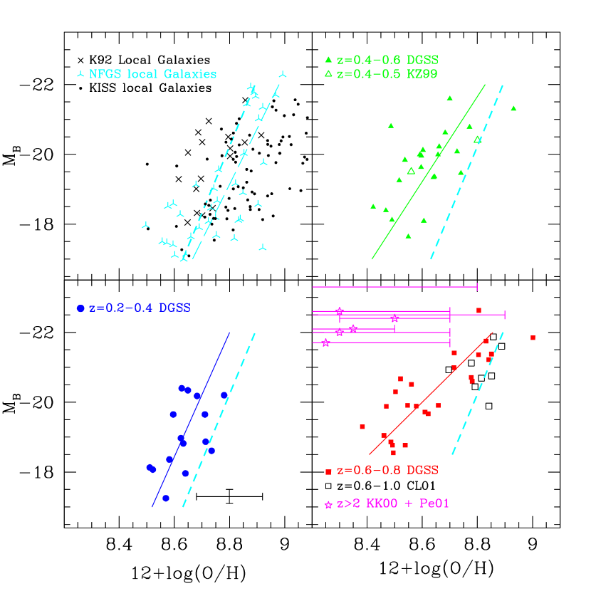
Figure 6: Luminosity-metallicity (L-Z) relation as a function of redshift including samples of local $z<0.1$ galaxies from the NFGS, KISS, and Kennicutt (1992b) catalogs, with intermediate-redshift DGSS objects from this study (filled symbols) and the Carollo & Lilly (2001) and Kobulnicky & Zaritsky (1999) compilations (open symbols). A representative error bar illustrating DGSS uncertainties on DGSS data is shown. Stars denote high-redshift objects (Kobulnicky & Koo 2000; Pettini et al. 2001) with error bars representing the full permitted range of metallicities. Lines show the best-fit relations including errors on both axes. The heavy dashed line in each panel is the fit to local K92 and NFGS galaxies. The long-dashed line in the upper left is the fit to all K92, NFGS, and KISS galaxies. Table 3 lists the details of the fit for each subsample. The L-Z relation based on the DGSS galaxies is increasingly offset from the local one with increasing redshift.

Figure 6 shows the best-fit luminosity-metallicity relation for DGSS galaxies compared to the three local galaxy samples. Filled symbols denote DGSS galaxies in the redshift ranges $z=0.26-0.4$, $z=0.4-0.6$, and $z=0.6-0.82$ as in Figure 5. Crosses, skeletal triangles and dots denote the K92, the NFGS and the KISS local samples, respectively. The eight open squares show the best-measured objects in the $0.6<z<1.0$ field galaxy study by Carollo & Lilly (2001; CL01). Open triangles show the $z=0.2-0.5$ objects from Kobulnicky & Zaritsky (1999; KZ99) which meet the same emission line selection criteria as the DGSS. Open stars are the high-redshift ($z>2$) galaxies from Kobulnicky & Koo (2000; KK00) and Pettini et al. (2001; Pe01). Lines represent linear least squares fits to each sample, taking into account the uncertainties on both O/H and $M_{B}$. Becuase errors on $M_{B}$ are usually smaller than the errors on O/H, this fit approaches a fit of metallicity on luminosity. In the upper left panel of local galaxies the long-dashed line marks the fit to the combination of all three local samples (K92+NFGS+KISS) while the heavy dashed line shows the fit to just the K92+NFGS data. Formal results from these fits and uncertainties appear in Table 2. The local galaxy samples were fit both collectively and then individually because they exhibit different distributions. The KISS galaxies lie preferentially to the right (metal-rich and underluminous) side of the best-fit L-Z relation for the combined K92+NFGS+KISS sample. One possible explanation for this offset is that KISS spectra were obtained with 2-3^′′ fibers or slits centered on the nucleus of each galaxy. Spectra dominated by emission from the inner several kpc will preferentially sample the metal-rich nuclei of galaxies and bias the KISS sample toward higher metallicities. For this reason, we use only the fit to the K92+NFGS samples (heavy dashed line in Figure 6) for comparison to the DGSS galaxies.

Figure 6 shows a representative error bar in the lower left panel indicating the typical statistical uncertainties of $\sigma(M_{B})=0.2$ mag and $\sigma(O/H)=0.10$ dex. It is worth emphasizing here that the oxygen abundances for all samples represented in Figure 6 have been computed in an identical manner from measured emission line equivalent widths. No corrections for internal reddening have been made. We have adopted the recommendation of KP03 and increased all local and DGSS galaxy $H\beta$ equivalent widths for 2 Å of stellar Balmer absorption. The absolute B magnitudes have been computed (or converted from published values) assuming the $H_{0}=70$, $\Omega_{M}=0.3$, $\Omega_{\Lambda}=0.7$ cosmology. K-corrections have been applied to the high-redshift samples based on multi-band rest-frame B-band and UV photometry. The various samples represented should be directly comparable, although they might not be completely representative of the entire population of galaxies at that redshift.

Figure 6 reveals a striking evolution in the slope and zero point of the best fit luminosity-metallicity correlation with redshift. This offset between local and DGSS samples is similar even if other fitting schemes are adopted (e.g., unweighted fits, or O/H errors only). Although considerable scatter exists within a given sub-sample, the more distant galaxies are markedly brighter at a fixed oxygen abundance. Alternatively, galaxies of a given luminosity are systematically more metal-poor at higher redshifts. The best fit relation for the local K92+NFGS samples is $12+log(O/H)=(-0.052\pm 0.009)~{}M_{B}+7.74$. For the $z\sim 0.7$ DGSS galaxies, we find $12+log(O/H)=(-0.128\pm 0.012)~{}M_{B}+6.04$. Note that these slopes differ considerably from other published L-Z relations for local galaxies. Melbourne & Salzer (2002), for example, find $12+log(O/H)=-0.24~{}M_{B}+4.0$. Some of this difference is due to the different metallicity calibrations used in that work compared to our study. The majority of the difference is due to the restricted range of galaxy luminosities and metallicities in the present DGSS sample. Melbourne & Salzer (2002) included all KISS galaxies on both halves of the doubled-valued $R_{23}$ to O/H relation, down to magnitudes of $M_{B}=-13$. They find evidence for a change in slope of the L-Z relation at low luminosities which alters the slope of their overall fit compared to that for our more restricted luminosity range.

More important than the formal zero point differences of the fits are the luminosity and metallicity offsets of the L-Z relation near the midpoints of the sample distributions. These midpoints are approximately at a metallicity of $12+log(O/H)\sim 8.7$ and a magnitude of $M_{B}=-20$. The low-redshift DGSS ($0.2<z<0.4$) subsample is as much as 1.6 magnitudes brighter and/or 0.10 dex more metal-poor than the mean of the local sample. The intermediate- and high-redshift DGSS subsamples are 2.0 and 2.4 magnitudes brighter than the local samples of similar luminosity and/or as much as 0.15 dex more metal-poor. High-redshift $z\sim 3$ galaxies show a larger offset of at least 3 magnitudes compared to the local sample, although the uncertainties on O/H are large for those objects. In the highest redshift DGSS bin, there is a statistically significant change in the best-fit slope of the L-Z relation in the sense that the least luminous galaxies at $0.6<z<0.8$ are more offset from the local L-Z relation compared to their more luminous counterparts at the same redshift.

Figure 6 shows that there is considerable dispersion among the local samples, such that some of the brightest, most metal-rich local galaxies overlap the $0.6<z<0.8$ L-Z relation. At luminosities fainter than $M_{B}=-19$, however, local galaxies are all 1-3 magnitudes fainter, for a given metallicity, compared to the $0.6<z<0.8$ objects. The change in slope of the L-Z relation at $0.6<z<0.8$ is in the sense that the low-luminosity DGSS galaxies in this redshift interval show greater offsets from the local samples than the high-luminosity galaxies. The lack of DGSS galaxies in the lower right corner of the plot (low luminosity but high metallicity) represents a real offset from the local relation and is not due any selection effect we can identify. Galaxies that might occupy this locus near $M_{B}=-19$, $12+log(O/H)=8.7$ would have measurable emission lines and line ratios, $R_{23}$, identical to the more luminous galaxies with $M_{B}=-21.5$. Although the ratios of [O III] and [O II] line strengths to H$\beta$ line strengths drop with increasing metallicity, the sample selection process would not preferentially exclude objects with low [O III]/H$\beta$ (high metallicity) in favor of those with high [O III]/H$\beta$ (low metallicity). If such low-luminosity, high-metallicity objects existed, they would have been detected and included in the analysis. In our selection of objects from the DGSS database, we found only 3 objects (at $z=0.36,z=0.76,z=0.77$) with measurable $H\beta$ but immeasurably weak [O III] (S/N$<8:1$). In all those cases, poor sky subtraction is clearly the cause of the weak [O III]. Furthermore, there is no correlation between $EW_{H\beta}$ and O/H (see Figure 5), as might be expected if selection effects had preferentially removed objects with weak line strengths from the sample or if the corrections for Balmer absorption dominated the errors in a systematic way. Although other selection effects in the local or distant samples may give the appearance of luminosity-metallicity evolution from $z=0.8$ to the present, we proceed in the next section to show that we can rule out several obvious selection biases.

3.3 Examination of Systematics with Color and Equivalent Width

Selection biases in the local and distant galaxy samples could produce the signature of an evolving L-Z relation seen in Figure 6. For instance, comparing local galaxies having moderate $EW_{H\beta}$ to the rare DGSS galaxies with strong starbursts and uncommonly large $EW_{H\beta}$ values could lead to misleading conclusions about the nature of distant versus local populations. We investigated sources of selection bias by examining the residuals in the L-Z relation as a function of other fundamental galaxy parameters. Using unweighted linear least-squares fits to the KISS, NFGS, and DGSS samples separately, we computed residuals for each sample and searched within each sample for correlations with galaxy color, $H\beta$ luminosity, size, and equivalent width. Only $EW_{H\beta}$ is marginally correlated with L-Z residuals, and only for the DGSS galaxies.

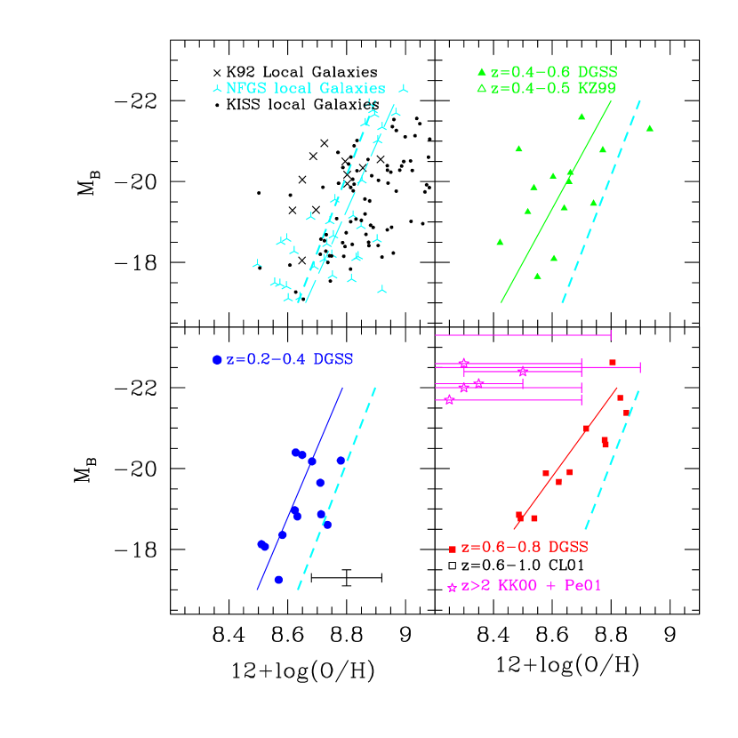
Figure 8: Luminosity-metallicity (L-Z) relations showing only local and DGSS galaxies with $EW_{H\beta}<20$ Å. The mean L-Z relations for the local and distant samples fitted here are essentially unchanged compared to the full set of galaxies in Figure 6, indicating that emission line EW differences between the local and DGSS samples are not responsible for the observed offsets in the luminosity-metallicity relation. Here again, DGSS galaxies are $\sim 1-2$ mag brighter than local galaxies of comparable metallicity.

Figure 7 plots galaxy $EW_{H\beta}$ versus luminosity residuals, $\delta{M_{B}}$, from the above best-fit linear relation for each subgroup in the L-Z plane. There is no correlation for the KISS sample or for the NFGS sample. We find a small trend for the highest-redshift DGSS galaxies which is driven by the handful of galaxies with extreme values of $EW_{H\beta}$, but the correlation coefficient indicates an equal or greater correlation could be achieved in a random sampling of points at least 20% of the time. The lack of a significant correlation between magnitude residuals and $EW_{H\beta}$ is evidence against the hypothesis that extreme starbursts, which temporarily increase the emission line strength and overall luminosity, are a source of dispersion in the L-Z relation. Hence, the larger emission line equivalent widths in the DGSS samples compared to the local samples do not bias the distant galaxies toward larger luminosities and are not responsible for the observed L-Z relation offsets. Further evidence for this conclusion comes from Figure 8, which shows only those DGSS and local KISS, NFGS, and K92 galaxies with the restricted EW criterion $EW_{H\beta}<20$ Å. Best fit lines to each sample show that the basic conclusion remains the same: distant DGSS galaxies are 1-2 magnitudes more luminous than local galaxies of comparable metallicity. This result does not appear to be due to some kind of selection effect since the DGSS sample analyzed here spans the entire range of luminosities from the entire DGSS sample in each redshift interval, i.e., we are not simply selecting the brightest objects from each redshift interval, as shown by Figure 3.

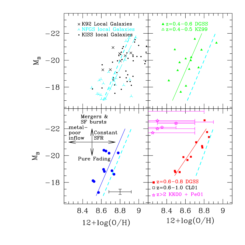
Figure 9: Luminosity-metallicity (L-Z) relation showing only local and DGSS galaxies with $B-V<0.6$ and $EW_{H\beta}<20$ Å. The best fit L-Z relations here are nearly unchanged from the previous plots, indicating that color and emission line EW differences between the local and DGSS samples are not responsible for the offsets in the luminosity-metallicity relation. The schematic in the lower left panel indicates the evolution in the L-Z plane caused by constant star formation, passive evolution, metal-poor gas inflow, and star formation bursts and/or galaxy mergers. If DGSS galaxies evolve into disklike star-forming galaxies today, then some combination of these processes are responsible for evolving the $z=0.6-0.8$ galaxies into the region occupied by today’s $z=0$ galaxies.

Figure 3 hints at another kind of selection effect which may lead to erroneous conclusions regarding differences between DGSS and local galaxy samples. All of the DGSS galaxies have very blue colors with $B-V<0.6$, while only a small fraction of local galaxies are as blue. The DGSS samples are likely to contain a larger fraction of extreme star-forming galaxies with younger light-weighted stellar populations. As a second means of examining selection/population differences between the local and DGSS samples, we have constructed a third version of Figure 6 using only local galaxies with the bluest colors. Figure 9 shows only those DGSS and local K92, KISS, and NFGS galaxies with $B-V<0.6$ and $EW_{H\beta}<20$ Å. Although the number of NFGS and KISS data points are fewer, best fit lines to each sample and the basic conclusions remain the same. Another way to look at this result is to say that the $0.6<z<0.8$ galaxies are 10% to 80% (0.04 to 0.25 dex, depending on $M_{B}$) more metal-poor than local galaxies of comparable luminosity. Selection effects such as differences in color distributions or EW distributions between the local and DGSS samples do not appear to be responsible for the observed variation of the L-Z relation with epoch.

3.4 Evolution of the L-Z Relation

One straightforward interpretation of Figure 6, Figure 8, and Figure 9 is to say that emission line galaxies have undergone considerable luminosity evolution, $\Delta M_{B}\simeq 1-3$ mag, from $z\sim 0.8$ (7 Gyr ago) to the present and as much as $\Delta M_{B}\simeq 3-4$ mag since $z\sim 3$ (11 Gyr ago). This amount of brightening is consistent with, or greater than than, the interpretation of Tully-Fisher evolution studies out to $z\sim 1$ (e.g., Forbes, 1995; Vogt et al. 1997; Simard & Pritchet 1998; Ziegler et al. 2002). An alternative way of understanding our new result is to say that emission-line field galaxies have experienced a measurable degree of metal enrichment (up to a factor of 2.0 for the least luminous objects) at constant luminosity since $z\sim 0.8$. The arrows in Figure 9 indicate evolution in the L-Z plane caused by constant star formation, passive evolution, metal-poor gas inflow, and star formation bursts and/or galaxy mergers. Constant star formation drives galaxies mainly to the right in Figure 9 (i.e., metal enrichment at constant luminosity) while passive evolution moves galaxies downward (i.e., fading at constant metallicity). Some combination of these two processes are probably responsible for evolving the $z=0.6-0.8$ galaxies into the region occupied by today’s $z=0$ galaxies, provided that the evolved descendants of the DGSS sample can be found among the local samples. Given that many of the DGSS galaxies appear to be disklike systems with active star formation, it is reasonable to suppose that a significant fraction of them are still disklike star-forming systems at the present epoch.

The apparent evolution in the luminosity-metallicity relation seen in Figures 6 and 9 stands in contrast to the conclusions of Kobulnicky & Zaritsky (1999) and Carollo & Lilly (2001), who found little or no evolution in the redshift ranges $0.1<z<0.5$ and $0.5<z<1.0$, respectively. Open squares in Figure 6 show that the CL01 objects fall at the high-luminosity end of the luminosity-metallicity correlation where the local and “distant” samples overlap. A comparison of the CL01 objects to the local samples and to the brightest DGSS galaxies shows that they have luminosities and metallicities similar to our most luminous objects and are consistent with the L-Z relation at that epoch. There is very little difference between the L-Z relations at $0.6<z<0.8$ and $z=0$ at the luminous end. Hence, the conclusion of CL01, namely that their galaxies lie near the L-Z relation for local galaxies, is appropriate given the restricted magnitude range of that sample. The new conclusion based on Figure 6 is made possible by the addition of larger numbers of lower-luminosity galaxies which greatly extend the luminosity and metallicity baselines. Although the Kobulnicky & Zaritsky (1999) sample included a broad range of luminosities, the least luminous objects were at the lowest redshifts where offsets from local galaxies are least pronounced. Furthermore, Kobulnicky & Zaritsky (1999) used a local comparison sample that included only a restricted subset of galaxies from the Kennicutt (1992a,b) spectral atlas. Objects from this sample show increased scatter toward low metallicities at fixed luminosity, due mostly to the errors introduced by variable, unknown amounts of stellar Balmer absorption. The increased scatter in the local sample masked the trend which has now become apparent in Figure 6. The global shift and slope change of the L-Z relation between $z=0$ and $z=0.8$ supports the conclusions of Kobulnicky & Koo (2000), Pettini et al. (2001) and Mehlert et al. (2002) at higher redshifts, who found galaxies to be overly luminous for their metallicity at $2.2<z<3.4$.

How do our results compare to conclusions about the evolution of the luminosity function (LF)? Lin et al. (1999) use early CNOC2 data on $>2000$ galaxies over the redshift range $0.12<z<0.55$ to conclude that, among late-type galaxies (the ones most comparable to the DGSS objects selected here), changes in the LF are most consistent with density evolution, and little or no luminosity evolution. However, Cohen (2002), based on studies in the Hubble Deep Field North vicinity over the redshift range $0.01<z<1.5$, concluded that emission-line objects show moderate luminosity evolution and little density evolution. Interpreting Figure 5 of Lin et al. (1999) as luminosity evolution suggests that, between $z\simeq 0.70$ and $z\simeq 0.20$, late-type galaxies with $M_{B}=-19$ fade by $\simeq$1 mag, while galaxies with $M_{B}=-21$ fade by $\simeq 0.2$ mag. More recent results of Wolf et al. (2002; COMBO-17 survey) show a decrease in the luminosity of $M^{*}$ galaxies from z$\sim 1$ to the present by as much as 2 magnitudes, dpending on spectral type. Given the uncertainties in the distant luminosity functions, this amount of fading is consistent with the amount of fading required for the $0.6<z<0.8$ DGSS galaxies to match the local L-Z relation in Figure 6. However, this consistency does not prove the fading model, and other possibilities are discussed below.

4 Discussion

4.1 Simple Galaxy Chemical Evolution Models

The addition of chemical information on galaxies at earlier epochs provides a new type of constraint on theories of galaxy formation and evolution. If local effects such as the gravitational potential and “feedback” from supernova-driven winds are the dominant regulatory mechanisms for star formation and chemical enrichment, then the L-Z relation might be nearly independent of cosmic epoch. The semi-analytic models of Kauffman (1996) and Somerville & Primack (1999) show little or no evolution in the L-Z relation with epoch, although uncertainties in the model-dependent prescriptions for stellar feedback and galactic winds may have large impacts on the computed chemical and luminous properties. Based on current understanding that the volume-averaged star formation rate was higher in the past (Pei & Fall 1995; Madau 1996), and that the overall metallicity in the universe at earlier times was correspondingly lower, we might expect galaxies to be both brighter and more metal-poor in the past. A high- or intermediate-redshift galaxy sample ought, therefore, to be systematically displaced from the local sample in the luminosity-metallicity (L-Z) plane if individual galaxies reflect these cosmic evolution processes. The key questions are two-fold: which dominates—the chemical evolution or luminosity evolution, and how do those rates differ, if they do, in low-luminosity galaxies versus high-luminosity galaxies? Comparison of the data from Figure 6 to some simple galaxy evolution models can help distinguish among these possibilities.

In a simple evolutionary model, galaxies begin as parcels of gas which form stars and produce metals as the gas fraction decreases from 100% to 0%. The B-band luminosity is related to the star formation history, which may vary as a function of time but is generally taken to be proportional to the mass or surface density of the remaining gas (e.g., Kennicutt 1998). For a galaxy that evolves as a “closed box”, converting gas to stars with a fixed initial mass function and chemical yield, the metallicity is determined by a single parameter: the gas mass fraction, $\mu=M_{gas}/(M_{gas}+M_{stars})$. The metallicity, $Z$, is the ratio of mass in elements heavier than He to the total mass and is given by

$$Z=Yln(1/\mu),$$ (9)

where $Y$ is the “yield” as a mass fraction. A typical total metal yield for a Salpeter IMF integrated over 0.2–100 $M_{\odot}$ is $Y=0.012$ by mass (i.e., 2/3 the solar metallicity of 0.018; see Pagel 1997, Chapter 8). A total oxygen yield for the same IMF would be $Y_{O}=0.006$. Effective yields in many local galaxies range from solar to factors of several lower (Kennicutt & Skillman 2001; Garnett 2002), implying either that the nucleosynthesis prescriptions (e.g., Woosley & Weaver 1995) are not sufficiently precise, that assumptions about the form of the initial mass function are incorrect, or that metal loss is a significant factor in the evolution of galaxies. Garnett (2002) finds that oxygen yields of $Y_{O}=0.001$ to $Y_{O}=0.014$ among local irregular and spiral galaxies are correlated with galaxy mass, suggesting an increasing amount of metal loss among less massive galaxies. High-velocity winds capable of producing mass loss are observed in local starburst galaxies (e.g., Heckman et al. 2000) and in high-redshift Lyman break galaxies (Pettini et al. 2001), but the actual amount of mass ejected from galaxies is difficult to estimate. Simulations indicate that winds may be metal-enriched, such that metals are lost from galaxies more easily than gas of ambient composition (Vader 1987; De Young & Gallagher 1990; MacLow & Ferrara 1999). Recent Chandra observations of a local dwarf starburst galaxy, NGC 1569, provide the first direct evidence for metal-enhanced outflows (Martin, Kobulnicky, & Heckman 2002). Thus, the closed-box models are probably not appropriate, and more realistic models including selective metal loss are required.

4.2 Comparison to Pégase2 Models

In order to compare the luminous and chemical evolution of galaxies in the L-Z plane to theoretical expectations, we ran a series of Pégase2 (Fioc & Rocca-Volmerange 1999) models. Pégase2 is a galaxy evolution code which allows the user to specify a range of input parameters. The critical input parameters include:

• $M_{tot}$: The total mass of gas available to form the galaxy. We explored a range of masses, and we present two representative masses of $10^{10}$ $M_{\odot}$ and $10^{11}$ $M_{\odot}$. No dark matter is included.

• $\tau_{infall}$: The timescale on which the galaxy is assembled. We assume that galaxies are built by continuous infall of primordial-composition gas with an infall rate that declines over an exponential timescale, $\tau_{infall}$, as implemented in Pégase2,

  $$M(t)=M_{tot}{{e^{-t/\tau_{infall}}\over{\tau_{infall}}}}.$$ (10)

  We chose two representative gas infall timescales of $\tau_{infall}=1$ Gyr and $\tau_{infall}=$5 Gyr.

• $\alpha(IMF)$: The form of the stellar initial mass function. We adopt the Salpeter value, $\alpha=-2.35$, between 0.1 and 120 $M_{\odot}$ (following Baldry et al. 2002).

• $Y$: The chemical yields from nucleosynthesis. We assign Woosley & Weaver 1995 B-series models for massive stars. The effective metal yield of these models is $Y=0.016$. The Pégase2 models treat a galaxy as a single zone with uniform chemical composition. This oversimplification is adequate to achieve a basic understanding of how fundamental parameters like star formation rate and gas supply affect gross galaxy properties like luminosity and metallicity, but it is insufficient for a detailed analysis of large galaxies with a range of internal metallicities.

• $F(SFR)$: The form of the star formation rate. We adopt a physically motivated prescription where the star formation rate is proportional to the mass of accumulated gas (or the gas density; Schmidt 1959; Kennicutt 1998).

• $A_{V}$: Extinction due to dust. We included an inclination-averaged extinction prescription as implemented in Pégase2, but extinction changes the model B magnitudes by only 0.2 mag. Extinction is of minor importance in the present comparison.

• $T_{0}$: The time after the Big Bang that a galaxy begins to assemble. While not explicitly part of the Pégase2 models, this parameter is implicitly required to match the ages of Pégase2 galaxies to a particular redshift and lookback time for our adopted cosmology. We initially assume that galaxies begin to form 1 Gyr after the Big Bang so that local $z=0$ galaxies have approximate ages of 12 Gyr (in a 13.5 Gyr old universe) and DGSS galaxies in our high-redshift bin at $0.6<z<0.8$ have ages of 5.7–6.5 Gyr (6.8–5.8 Gyr lookback times). For convenience, Table 3 lists the lookback time and age of the universe at a given redshift for our adopted cosmology. We show later that allowing a range of $T_{0}$ provides a natural explanation for some of the features seen in the L-Z relations.

Our goal in the Pégase2 modeling was to reproduce the qualitative behavior of Figure 6 where, 1) galaxies at $0.2<z<0.8$ are displaced toward brighter magnitudes and/or lower metallicities relative to their $z=0$ counterparts, and 2) DGSS galaxies at $0.6<z<0.8$ exhibit a change in slope compared to more local L-Z relations. A significant constraint on the models is the position of $z\simeq 3$ Lyman break galaxies, which lie 2-4 magnitudes brighter (0.5 dex more metal-poor) than the local L-Z relation. If the present-day emission-line samples are at all representative of the evolved descendants of the $0.6<z<0.8$ and $z\simeq 3$ galaxies, then a successful model must reproduce the rapid rise in metallicity and luminosity in the first 2-3 Gyr (as evidenced by the Lyman break galaxies), and it must reproduce the lack of significant L-Z evolution during the past 2-3 Gyr (as evidenced by the similarity of the $z=0.2$ galaxies to the present-day L-Z relation). This means that the rate of evolution of the L-Z relation must be rapid during the first few Gyr of a galaxy’s formation, and it must then drop dramatically as a galaxy approaches the present-day L-Z relation. Furthermore, large luminous galaxies should slow their L-Z evolution more than less luminous galaxies. A slowing of the luminous and/or chemical evolution of a galaxy must physically correspond either 1) to cessation of star formation and ultimately to depletion of the gas available to fuel star formation, or 2) to continued inflow of metal-poor gas which fuels star formation and dilutes the composition of the ISM so that a galaxy remains fixed in L-Z space.

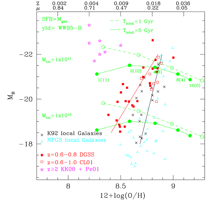
Figure 10: L-Z relation with a subset of the symbols from Figure 6. Lines show the $0.6<z<0.8$ (red) and local (black) L-Z relations from Figure 6. Curved tracks and and pentagons show the chemical and luminous evolution of Pégase2 model galaxies with a star formation rate proportional to the gas mass, where the galaxy is built by exponentially-decreasing infall of primordial gas with infall timescales of 1 Gyr and 5 Gyr. Pentagons denote galaxies at ages of 1, 2, 4, 8, and 12 Gyr (corresponding to lookback times, as shown in parentheses, of 11, 10, 8, 4, and 0 Gyr, respectively). Galaxy masses of $10^{10}$ $M_{\odot}$ and $10^{11}$ $M_{\odot}$ (neglecting dark matter) are shown. The top of the figure shows the corresponding gas metallicity, $Z$, and mass fraction, $\mu$, assuming a closed-box scenario for an effective yield of 0.016 from Weaver & Woosley (1995) series B models. These models match the observed rapid rise in gas-phase metallicity of Lyman break galaxies but overproduce metals today compared to observed galaxies.

Figure 10 shows evolutionary tracks of galaxies in the L-Z plane based on the infall Pégase2 models. The warm ISM metallicity by mass, $Z$, is marked along the upper $x$-axis along with the corresponding closed-box gas mass fraction given by the models (equivalent to the gas mass fractions predicted by Equation 9 using a total yield of $Y$=0.016) as a comparison. Pentagons in Figure 10 mark the model galaxies at ages of 1, 2, 4, 8, and 12 Gyr (from left to right). The numbers in parentheses next to each model point show the lookback time in Gyr assuming that the galaxy begins its assembly 1 Gyr after the Big Bang.

Dashed lines denote models with $\tau_{infall}=1$ Gyr and solid lines denote models with $\tau_{infall}=5$ Gyr. The upper set of curves shows galaxies with $M_{tot}=10^{11}$ $M_{\odot}$ while the lower curves show galaxies with $M_{tot}=10^{10}$ $M_{\odot}$(not including dark matter). Solid lines mark the best-fit L-Z relations from Figure 6. These models produce the rapid rise in metallicity in the first few Gyr. These model masses are in reasonable agreement with observational estimates which place lower limits on the dynamical masses of $z\simeq 3$ Lyman break galaxies at $few\times 10^{10}$ $M_{\odot}$ (Kobulnicky & Koo 2000; Pettini et al. 2001 and indicate star formation rates of $\sim$50 $M_{\odot}$/$yr^{-1}$. However, these models over-enrich the ISM at late times after 8 Gyr compared to the data. They predict gas mass fractions that are as low as 1% and metallicities as high as 3 times solar (Z=0.054) after 12 Gyr, at odds with the observed properties of nearby galaxy samples.

We can achieve better agreement between the models and data by varying several crucial model parameters.

• Varying the SFR: Lowering the model star formation rates would delay the chemical enrichment until later times and lower the luminosity at any given time. Effectively, this change produces a wholesale shift in the model curves to the left and downward in Figure 10. However, lowering the SFR would also lower the predicted emission line equivalent widths which may already be too low in the models compared to the data (mean of $EW_{H\beta}=10$ Å after 8 Gyr versus 15-20 Å in the data). Thus, changing the SFR does not improve the model agreement with the data.

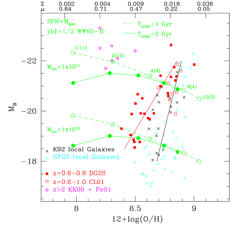
Figure 11: Comparison of data to evolutionary models in the L-Z plane similar to Figure 10, except that the effective yield of the models has been arbitrarily reduced by a factor of 2 ($\eta_{Z}=0.5$). Lines show the best-fit L-Z relations from Figure 6. Curved tracks and and pentagons show the evolution of a model galaxy with a star formation rate proportional to the gas mass where the galaxy is built by exponentially-decreasing infall of primordial gas with infall timescale of 1 Gyr and 5 Gyr, same as for the models in Figure 10. Pentagons denote galaxies at ages of 1, 2, 4, 8, and 12 Gyr (corresponding to lookback times, as shown in parentheses, of 11, 10, 8, 4, and 0 Gyr, respectively). Galaxy masses of $10^{10}$ $M_{\odot}$ and $10^{11}$ $M_{\odot}$ are shown. The metallicities of the reduced-yield models do not rise as quickly, do not overproduce metals at late times and are in overall better agreement with the data. Longer gas infall timescales for low-mass galaxies compared to high-mass galaxies gas is one way of reproducing the slope and offset variations of the local and distant L-Z relations. Later formation epochs for low-mass galaxies or reduced effective metal yields for low-mass galaxies will also serve to produce the change in slope and offset for the low-luminosity DGSS galaxies.

• Varying the chemical yield, $Y$: As an experiment to produce models that better resemble the data, we introduced a metal yield efficiency parameter, $\eta_{Z}$, which reduces the effective yield of the models. Reducing the chemical yields simply moves the model curves en masse to the left without changing the spacing of the model points (i.e., without changing the $\Delta(O/H)$ over a fixed time interval). Physically, $\eta_{Z}$ may represent the fraction of metals retained in galaxies during episodes of wind-driven metal loss, or it may represent a correction to the theoretical yields from stellar populations. Figure 11 shows the same models and data as Figure 10, except that the metal yield has been reduced to 1/2 ($Y_{O}=0.003$ for $\eta_{Z}=0.5$). The $M_{tot}=10^{11}$ $M_{\odot}$ model with $\tau_{infall}=1$ Gyr is now in better agreement with the $0.6<z<0.8$ and $z=0$ data at ages of 8-12 Gyr. However, the same model for $M_{tot}=10^{10}$ $M_{\odot}$ becomes too metal-rich at ages of 8-12 Gyr compared to the $z=0$ data.

• Varying $\tau_{infall}$: Increasing the infall timescale from 1 Gyr to 5 Gyr, as shown in Figure 11, alters a galaxy’s evolution in several respects. It significantly decreases the luminosity during the first few Gyr, while producing a slight drop in the gas-phase metallicity at each timestep. Longer $\tau_{infall}$ also decreases the change in metallicity in each timestep, i.e., decreases the $\Delta(O/H)$ over a fixed time interval, most noticeably at late epochs. In the context of the cold dark matter paradigm, the objects with the largest initial overdensities form most rapidly (e.g., Blumenthal et al. 1984; Navarro, Frenk, & White, 1995). Whether these first objects grow to become massive galaxies depends on the environment in which they are conceived. Initial galaxy cores which collapse in the vicinity of larger concentrations of baryonic matter grow to become the massive galaxies at the centers of today’s galaxy clusters. Objects that form in regions of lower cosmological overdensity would accrete gas on longer timescales and, if isolated from external influences, would proceed more slowly through the star formation and chemical evolution process. A longer formation timescale for lower mass field galaxies observed in the DGSS at $0.6<z<0.8$ can plausibly explain their observed evolution in the L-Z relation. Figure 11 demonstrates that $\tau_{infall}=5$ Gyr provides better agreement than the $\tau_{infall}=1$ Gyr to the $0.6<z<0.8$ and $z=0$ galaxies. However, we stress that a single set of model parameters cannot reproduce either the L-Z relation itself at any epoch or the variation in slope of the L-Z relation with epoch. The L-Z relation predicted by a single set of model parameters at any epoch would be a vertical line in Figure 11!

• Varying $T_{0}$: Delaying the epoch at which model galaxies begin to assemble simply relabels the ages of models. For example, setting $T_{0}=2$ Gyr instead of $T_{0}=1$ Gyr renumbers the ages of the model points in Figure 11 from 1,2,4,8,12 Gyr to 0,1,3,7,11 Gyr. For a given lookback time, the galaxies are younger.

The effects of decreasing $Y$, increasing $\tau_{infall}$, and increasing $T_{0}$ are, to some degree, degenerate. They all serve to move model points toward the left (metal-poor) side of Figure 11, and we cannot, here, discriminate between their relative importance. However, within the context of these simple models, no single parameter can solely explain both the slope of the L-Z relation and the change in slope with lookback time. These observed qualities can only be produced in the context of the Pégase2 models if at least two of the following conditions obtain: 1) the chemical yield of low-luminosity galaxies are reduced relative to high-luminosity galaxies (e.g., Garnett 2002), 2) $\tau_{infall}$ is larger for low-luminosity galaxies relative to high-luminosity galaxies, 3) $T_{0}$ is larger for low-luminosity galaxies relative to high-luminosity galaxies (e.g., as in the delayed formation scenarios for dwarfs, Babul & Rees 1992). Such a scenario, whereby galaxies assembly timescales or formation epochs vary with environment, is similar to that proposed by Sandage, Freeman, & Stokes (1970) to explain the differences along the Hubble sequence.

There is considerable observational support for the idea that lossy galactic winds remove metals and reduce the effective chemical yields from star formation (e.g., Martin, Kobulnicky & Heckman 2002; Garnett 2002). Winds are more effective in low-mass galaxies with lower gravitational potentials. The overall slope of the L-Z relation may plausibly be explained by a decreasing effective yield in low-luminosity (low-mass) galaxies. Some combination of longer $\tau_{infall}$, and/or later $T_{0}$ for low-mass galaxies may then be invoked to explain the change in slope of the L-Z relation which preferentially displaces $0.6<z<0.8$ low-luminosity galaxies more dramatically from the local L-Z relation.

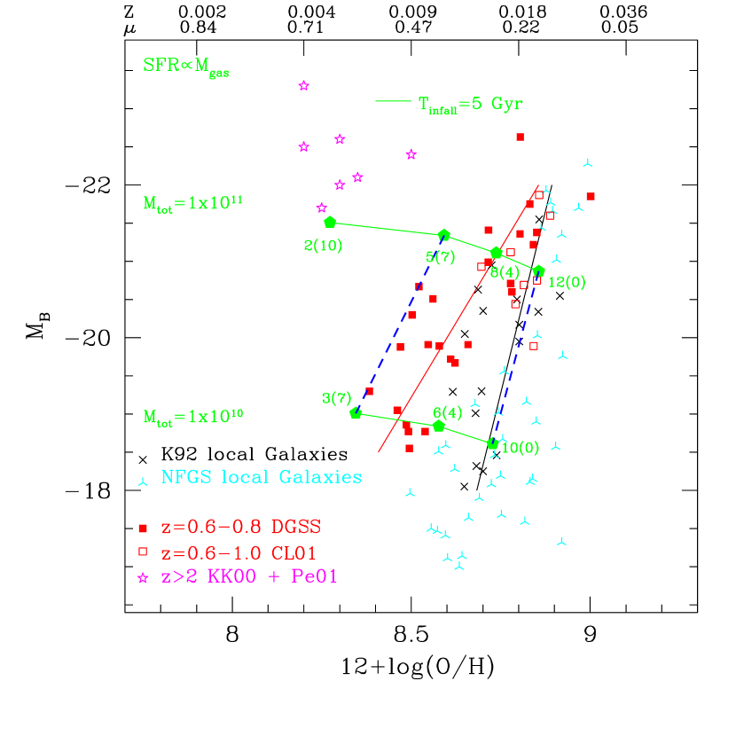
Figure 12: Comparison of data to evolutionary models in the L-Z plane similar to Figure 11, except that the effective yield of the $10^{10}~{}M_{\odot}$ model has been arbitrarily reduced by an additional factor of 20% relative to the $10^{11}~{}M_{\odot}$ model to simulate the impact of increasingly efficient galactic winds in lower mass galaxies. Lines show the best-fit L-Z relations from Figure 6. Here, the model points are labeled with age (and lookback times in parentheses) assuming that the $10^{11}~{}M_{\odot}$ galaxy begins assembly at $T_{0}=1$ Gyr and that the $10^{11}~{}M_{\odot}$ galaxy begins assembly at $T_{0}=3$ Gyr. Heavy dotten lines (blue) connect model points at the same lookback time. The combined effects of decreased yield and later formation epoch for the lower mass galaxy qualitatively simulates both the slope of the L-Z relation and the change in slope and offset of the L-Z relation at earlier epochs. However, the models slightly underpredict the chemical enrichment observed in galaxies at $0.6<z<0.8$, and they do a poor job of predicting the evolution of luminous galaxies.

Figure 12 uses the same Pégase2 models to explore how one possible combination of reduced metal yields in low-mass galaxies relative to larger galaxies combined with a later formation epoch for low-luminosity galaxies, can come close to reproducing both the slope of the L-Z relation and its zero point and slope variations with redshift. Solid lines show the 5 Gyr infall models from previous figures. As in Figure 11, we use $\eta_{Z}=0.5$ for the $10^{11}$ $M_{\odot}$ galaxy but here we choose $\eta_{Z}=0.4$ for the $10^{10}$ $M_{\odot}$ galaxy. This variation in yield is well within the range found by Garnett (2002). For the $10^{11}$ $M_{\odot}$ galaxy we adopt a formation epoch $T_{0}=1$ Gyr while for the $10^{10}$ $M_{\odot}$ galaxy we choose a formation epoch $T_{0}=3$ Gyr. The numbers next to each model point denote the lookback time and the numbers in parentheses denote galaxy age. Note how the slope of the L-Z relation is in good agreement with a line connecting the model points at the present epoch, but it is in good rather poor with the slope of a line connecting the model points at a lookback time of 7 Gyr (roughly $0.6<z<0.8$). Moreover, the DGSS galaxies at $0.6<z<0.8$ are, as a whole, more metal-rich than the model points at 7 Gyr lookback times, indicating that these particular Pégase2 models fail to reproduce (i.e., they overpredict) the magnitude of zero-point evolution in the L-Z relation. Nevertheless, this combination of later formation epoch and reduced yield for low-mass galaxies does a reasonable job of reproducing the sense of the zero point and slope evolution in the L-Z plane with redshift, especialyl for the low-luminosity galaxies. The largest discrepancies are for luminous galaxies whose gas-phase metallicity evolves less than the Pégase2 models predict.

4.3 Limitations of the Single-Zone Pégase2 Models

As noted, the single-zone Pégase2 models in the above figures fail to reproduce one important feature of the L-Z relation data, namely, the observed lack of evolution for luminous galaxies between $0.6<z<0.8$ and $z=0$. All of the models in Figures 10,11, and 12 predict an increase of 0.2 – 0.4 dex in O/H between lookback times of $\sim 7$ Gyr and the present. Yet, the linear fits to the local and the $0.6<z<0.8$ DGSS data indicate get little ($<0.1$ dex) change in O/H for the most luminous galaxies ($M_{B}<-21$). The only ways to decrease the $\Delta(O/H)$ per timestep withinthe framework of these single-zone models are 1) to drastically reduce the star formation rate, i.e., to slow the conversion of gas into stars and heavy elements, or 2) to increase the infall timescale beyond the 5 Gyr models. However, such a decrease in star formation rate or increase in $\tau_{infall}$ would produce model galaxies which are dramatically more metal-poor and gas-rich at a given age compared to the present models, and would be in poor agreement between the models and the data. We can find no reasonable range of Pégase2 model parameters which reproduce the similarity of luminous local galaxies to $0.6<z<0.8$ luminous DGSS galaxies.

The resolution to this crisis may lie in the considerable internal complexity of large spiral galaxies (e.g., radial chemical gradients, spatially variable extinction and star formation rates), which single-zone model like Pégase2 do not include. More sophisticated models which treat galaxies as a collection of annuli with differing gaseous and chemical properties, for example, might more accurately reproduce the observed characteristics of the large galaxies seen locally and in the DGSS. The lack of L-Z evolution among luminous galaxies in Figure 11 might be explained if star formation and chemical enrichment in these objects proceeds radially from the inside-out. If the star formation in local galaxies is dominated by activity at a larger radius than the star formation activity in $0.6<z<0.8$ DGSS galaxies, then the luminosity-weighted DGSS spectra will preferentially reflect the chemical composition at different (i.e., smaller) galactocentric radii in DGSS galaxies than in local galaxies. Although local luminous spiral galaxies may, on whole, be substantially more metal-rich today than at $0.6<z<0.8$, their emission line luminosities today would be dominated by star formation in comparably-enriched regions, but at larger radii, compared to the DGSS galaxies. Observations of the mean star formation radius within disk galaxies as a function of redshift could test this hypothesis. Regardless of whether this particular hypothesis is true, additional information about the spatial distribution of star forming regions in distant objects (e.g., using the Hubble Space Telescope), will lead to a greater understanding of the luminous and chemical histories of large galaxies.

One additional free parameter not incorporated into the Pégase2 models is the role of starbursts on timescales of a few Myr that occur in galaxies that evolve on long (Gyr) timescales according to the model prescriptions above. Studies of local galaxies show that their star formation histories are not smooth but instead are punctuated by periods of enhanced activity. Such short-term enhancements in the star formation rate of galaxies otherwise evolving smoothly can elevate the luminosity and emission line equivalent widths by factors of several. The observed emission line equivalent widths in DGSS galaxies average 10-20 Å, but some exceed 50! These characteristics would be better fit by superimposing a burst of star formation of $\sim 10^{6-7}$ $M_{\odot}$ on the model galaxies. The impact of instantaneous bursts on the evolution in the L-Z plane would be to create spikes along the model tracks toward higher luminosities. The amplitude of the spikes would scale with the amplitude of the burst, and could conceivably be up to several magnitudes and would persist up to a few 100 Myr. Given the morphological evidence for ongoing mergers among the DGSS sample, evidenced by inspection of Figure 1, it seems possible that short-term enhancements in the star formation rate are responsible for the more extreme luminosities and emission line equivalent widths among the sample. Examination of the Pégase2 models used here shows that as the $EW_{H\beta}$ declines from 50 Å to 10 Å, the B-band luminosity drops by 0.7 mag. If we were to try to correct the magnitudes of the DGSS samples by some factor to account for their larger equivalent widths compared to the local samples, this factor would be less than 0.7 mag, not enough to account fully for the larger 1-2 mag offsets observed in the L-Z relations. This is further evidence against the possibility that the offset of the L-Z relation at $z=0.7$ is merely caused by starbursts with temporarily elevated luminosities and equivalent widths, although this may be part of the answer.

5 Conclusions

Observations of star-forming galaxies from the Deep Extragalactic Evolutionary Probe (DEEP) survey of Groth Strip galaxies in the redshift range $0.26<z<0.82$ show a correlation between B-band luminosity and ISM oxygen abundance, like galaxies in the local universe. Both the slope and zero-point of the L-Z relation evolve with redshift. DGSS galaxies are 1—3 mag more luminous at $0.6<z<0.8$ than $z=0$ galaxies of similar metallicity. Said another way, galaxies of comparable luminosity are 0.1-0.3 dex more metal-rich at $z=0$ compared to $0.6<z<0.8$. The change in slope of the L-Z relation is most pronounced for DGSS galaxies at $0.6<z<0.8$ and indicates that the apparent chemo-luminous evolution is more dramatic for the least luminous galaxies. We have ruled out several selection effects and biases in the galaxy samples which could produce this result. Evolution of galaxies in the L-Z plane over the redshift range $z=3$ to $z=0$ appears to result from a combination of fading and chemical enrichment for plausible single-zone galaxy evolution models. Within the context of these models, the slope of the L-Z relation and the observed evolution of slope and zero-point with redshift imply that that at least two of the following are true for star-forming galaxies out to $z\simeq 0.8$: 1) low-luminosity galaxies have lower effective chemical yields than massive galaxies, 2) low-luminosity galaxies assemble on longer timescales than massive galaxies, 3) low-mass galaxies began the assembly process at a later epoch than massive galaxies. Comparison of observed ISM metallicities to simple galaxy evolution models suggests that loss of up to 50% of the oxygen is necessary to avoid over-enriching the galaxies at the observed redshifts. While the models do a reasonable job of reproducing the evolution of the less luminous galaxies in our sample ($M_{B}\sim-19$), the models do a poor job of reproducing the relative lack of chemo-luminous evolution seen among the luminous galaxies in our sample ($M_{B}\sim-22$), suggesting a breakdown of the single-zone approximation. We predict that DGSS galaxies have significantly higher (20%-60%) gas mass fractions than comparably luminous local galaxies. Such a systematic difference in the mean gas mass fractions of distant galaxies could, in principle, be observed with instruments such as the proposed radio-wave Square Kilometer Array.

Appendix A Applicability of $EWR_{23}$ Method to DGSS Galaxies

Kobulnicky & Phillips (2003) showed that the quantity $EWR_{23}$ is a good surrogate for the metallicity indicator $R_{23}$ over a wide range of galaxy colors and emission line properties. However, the correlation between $EWR_{23}$ and $R_{23}$ is tightest for galaxies with strong emission lines (e.g., $EW_{H\beta}>10$). Furthermore, the residuals from the 1:1 correspondence show a slight correlation with galaxy color, the residuals being smallest for the bluest galaxies. Figure 13 reproduces part of Figure 5 from KP03 and shows the distribution of $EWR_{23}$, $\log~{}EW_{H\beta}$, $\log~{}EW_{[O~{}II]}$, $\log~{}(EW_{[O~{}III]}/EW_{[O~{}II]})$, and $B-V$, (histograms) of 66 DGSS galaxies compared to the residuals from the $EWR_{23}$ vs. $R_{23}$ relation. This figure demonstrates that the DGSS galaxies studied here lie in regimes where the $EWR_{23}$ vs. $R_{23}$ correlation is strong and well-behaved. For these galaxies, $EWR_{23}$ is a good surrogate for $R_{23}$.

Figure 1: Unfluxed spectra for 66 emission-line galaxies culled from the DEEP survey of the Groth Strip using the criteria discussed in Section 2, along with their HST F814W images. Y-axis is counts in ADU where ADU=$e^{-}/2.4$. Objects are ordered by redshift, as in Table 1, with the 10 possible or probable AGN at the end. Markings identify major emission lines of the [O II]$\lambda$3726/29 doublet, [Ne III] $\lambda 3868$, H$\beta$, [O III]$\lambda\lambda$4959,5007, and, where applicable, $H\alpha$. Other positive features are generally residuals from night sky lines which could not be completely subtracted. Each panel shows two different spectra, obtained with “red” and “blue” grating settings. Seven-digit strings in the upper left give the DGSS identification number. Rectangles on the images show spectroscopic slit positions. (All 10 panels appear in the electronic edition only).

Figure 2: Histogram of 66 galaxies selected for chemical analysis (filled) compared to the total 398 objects in the survey with $0.26<z<0.82$. We show the distribution as a function of redshift, $M_{B}$, B-V color, half-light radius $R_{hl}$, bulge fraction $F_{bulge}$, and asymmetry index, $R_{T}+R_{A}$. This figure demonstrates that galaxies selected as suitable for chemical analysis are moderately representative of the larger DGSS sample in the same redshift range in terms of their redshift distributions, sizes, luminosities and bulge fractions. However, the 66 selected galaxies preferentially have bluer B-V colors and more asymmetric morphologies, consistent with higher rates of star formation.

Figure 3: A comparison of luminosity, color, and emission line strength for 64 galaxies selected for chemical analysis (solid symbols) to the 276 DGSS galaxies with emission lines (open symbols) selected from among the 398 DGSS galaxies in the three redshift bins spanning the $0.26<z<0.82$ range. Error bars show subsample means and dispersions. Galaxies selected for analysis in the lowest redshift bin are representative of the DGSS objects in that redshift interval. However, galaxies selected for analysis from the highest redshift bins are biased toward the bluest colors and highest emission line equivalent widths.

Figure 4: Relation between the emission line ratio, $\log R_{23}\equiv\log[(I_{3727}+I_{4959}+I_{5007})/(I_{H\beta})]$, and oxygen abundance, 12+log(O/H) for a variety of calibrations from the literature. We adopt an analytical expression for the upper branch of the McGaugh (1991) relation which takes into account the ionization parameter as measured by the $O_{32}$ ratio. Two values of $\log(O_{32})=1$ and $\log(O_{32})=0$ are shown. A star marks the Orion Nebula oxygen abundance (Walter, Dufour, & Hester 1992) which is within 0.02 dex of the recent solar abundance measurement by Prieto, Lambert, & Asplund (2001).

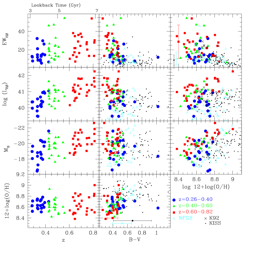
Figure 5: Relation between redshift, $M_{B}$, $B-V$ color, $EW_{H\beta}$, $L_{H\beta}$, and 12+log(O/H) for 64 DGSS galaxies with subsets of the local NFGS, K92, and KISS samples chosen to match the DGSS emission-line ratio selection criteria. Points with error bars in some panels compare the means and dispersions in color and $EW_{H\beta}$ for the DGSS, NFGS, and KISS samples. DGSS galaxies in the highest redshift bin are preferentially bluer with higher star formation rates and larger emission line equivalent widths. Each redshift interval exhibits a correlation between metallicity and both blue and $H\beta$ luminosities, but with different zero points. There is no significant correlation between metallicity and color, or between metallicity and emission line equivalent width.

Figure 7: Galaxy $EW_{H\beta}$ versus luminosity residuals, $\delta{M_{B}}$, from best-fit linear relations in the L-Z plane. DGSS subsampels are fitted individually using the relations of Table 2, while the the fit to the combined NFGS+KISS+K92 objects is used for those samples. Note that KISS residuals are systematically positive (faint) compared to the NFGS residuals. There is no correlation between $EW_{H\beta}$ and L-Z residuals for the local samples. There is only a weak correlation among the DGSS galaxies in the highest redshift bin, driven mostly by the few galaxies with extreme values of $EW_{H\beta}$. We searched for other parameters, including galaxy color and size, which might correlate with L-Z residuals and explain some of the dispersion in the L-Z relation, but no significant correlations were found. Dispersion in the L-Z relation is either intrinsic or attributable to a yet unidentified combination of parameters.

Figure 13: Comparison of the quantity $R_{23}$ with $EWR_{23}$ from Kobulnicky & Phillips (2003). The strong correlation between $R_{23}$ and $EWR_{23}$ (upper left panel) shows that oxygen abundances can be estimated from equivalent width ratios at least as well as from dereddened line fluxes. The RMS dispersion from the 1-to-1 relation is $\sigma(log[R_{23}])=0.07$ dex. Lower panels explore the residuals in the correlation as a function of line strength, line ratio, and galaxy color. Histograms in the right column show the distribution of colors and emission line strengths for the 66 emission-line galaxies selected for analysis from the DGSS. The majority of galaxies lie in regimes where the $EWR_{23}$ vs. $R_{23}$ correlation is strong and well-behaved.

Table 1: DGSS Selected Galaxies

ID	Object	RA (2000)	DEC (2000)	z	$I_{814}AB$	$M_{B}$	$(B-V)$	$R_{hl}$	$B/T$	$R_{T}$	$R_{A}$	$EW_{3727}$	$EW_{4861}$	$EW_{4959}$	$EW_{5007}$	$12+log(O/H)$	$SFR$	Notes
(1)	(2)	(3)	(4)	(5)	(6)	(7)	(8)	(9)	(10)	(11)	(12)	(13)	(14)	(15)	(16)	(17)	(18)	(19)
1	073-2658	14:17:47.597	52:29:03.36	0.2863	21.13	-18.9	0.34	2.88	0.28	0.04	0.10	62.1$\pm$1.6	10.8$\pm$1.1	11.1$\pm$2.2	23.0$\pm$1.2	8.62$\pm$0.11	0.7	A,B
2	072-2273	14:17:38.928	52:29:34.72	0.2888	22.03	-18.0	0.36	2.36	0.00	0.03	0.05	49.5$\pm$1.4	10.1$\pm$0.4	6.5$\pm$0.4	25.7$\pm$0.4	8.52$\pm$0.08	0.3	A
3	072-4040	14:17:37.838	52:28:58.44	0.2908	20.01	-19.6	0.70	9.42	0.00	0.15	0.06	26.9$\pm$1.1	5.9$\pm$0.3	1.7$\pm$0.2	5.7$\pm$0.2	8.71$\pm$0.08	1.0	A
4	172-1242	14:16:35.570	52:17:27.91	0.3288	24.22	-16.4	0.17	1.37	0.10	-.02	0.01	22.9$\pm$1.7	30.2$\pm$3.6	39.1$\pm$3.9	121$\pm$4	8.73$\pm$0.04	0.1	A,C
5	092-1375	14:17:26.699	52:27:19.48	0.3315	23.84	-16.6	0.39	1.54	0.15	0.06	0.04	22.8$\pm$1.2	12.6$\pm$0.7	13.2$\pm$0.7	32.5$\pm$0.7	8.75$\pm$0.03	0.1	A,C
6	134-2322	14:17:05.547	52:21:18.17	0.3319	21.28	-18.3	1.02	2.39	0.34	0.05	0.15	39.1$\pm$1.0	9.9$\pm$0.5	10.8$\pm$0.6	24.1$\pm$0.5	8.58$\pm$0.06	0.7	A
7	142-4644	14:16:51.341	52:20:52.38	0.3322	21.52	-18.8	0.47	3.62	0.00	0.03	0.01	76.1$\pm$1.2	19.2$\pm$1.6	6.9$\pm$1.9	30.5$\pm$2.1	8.63$\pm$0.09	1.2	A
8	223-2132	14:16:07.432	52:11:25.04	0.3359	23.16	-17.2	0.48	1.16	0.04	-.01	0.00	33.8$\pm$2.8	6.8$\pm$0.9	5.1$\pm$0.8	15.1$\pm$1.1	8.57$\pm$0.09	0.1	A
9	124-3864	14:17:14.790	52:21:50.38	0.3564	21.55	-18.8	0.56	3.02	0.00	0.05	0.07	34.2$\pm$3.3	7.2$\pm$0.5	0.8$\pm$0.7	2.5$\pm$0.5	8.71$\pm$0.10	0.5	A
10	173-5210	14:16:36.664	52:17:39.89	0.3570	20.03	-20.4	0.54	4.51	0.05	0.07	0.06	34.9$\pm$0.9	5.8$\pm$0.4	1.4$\pm$0.4	3.5$\pm$0.4	8.62$\pm$0.12	1.7	A
11	103-6061	14:17:27.434	52:26:08.93	0.3631	21.88	-18.6	0.51	0.93	0.49	0.03	0.01	38.9$\pm$0.7	10.9$\pm$0.6	4.4$\pm$0.5	11.3$\pm$0.5	8.74$\pm$0.07	0.6	A
12	203-4851	14:16:21.680	52:14:14.78	0.3639	22.58	-18.1	0.36	1.18	0.70	0.02	0.01	52.6$\pm$1.1	12.2$\pm$0.4	13.8$\pm$0.4	34.6$\pm$0.4	8.51$\pm$0.06	0.3	A
13	213-6640	14:16:13.664	52:13:20.44	0.3656	20.22	-20.3	0.50	4.62	0.03	0.06	0.05	26.2$\pm$3.2	4.2$\pm$0.3	0.5$\pm$0.3	0.8$\pm$0.3	8.66$\pm$0.15	0.9	A,B
14	313-3557	14:15:11.917	52:01:10.88	0.3757	20.56	-20.2	0.42	2.35	0.25	0.06	0.04	44.4$\pm$0.9	13.3$\pm$0.2	3.3$\pm$0.1	9.0$\pm$0.2	8.78$\pm$0.07	2.8	A
15	304-4028	14:15:17.787	52:01:23.63	0.3760	22.78	-17.9	0.41	1.38	0.02	0.03	0.04	99.5$\pm$1.1	27.8$\pm$1.3	14.6$\pm$1.6	46$\pm$1.6	8.64$\pm$0.07	0.7	A
16	183-6415	14:16:30.453	52:16:42.93	0.3865	21.00	-19.6	0.55	7.06	0.00	0.14	0.07	109$\pm$50.	24.2$\pm$2.5	8.3$\pm$2.5	27.8$\pm$2.7	8.60$\pm$0.12	3.6	A,B
17	193-5319	14:16:24.702	52:15:23.83	0.3929	20.62	-20.1	0.46	4.45	0.03	0.06	0.07	55.5$\pm$0.4	12.5$\pm$0.2	2.3$\pm$0.2	7.3$\pm$0.4	8.69$\pm$0.09	2.8	A
18	092-1962	14:17:26.421	52:27:06.04	0.4261	19.49	-21.5	0.40	6.35	0.03	0.20	0.15	24.4$\pm$0.2	4.8$\pm$0.2	1.0$\pm$0.1	4.3$\pm$0.1	8.68$\pm$0.09	3.3	A
19	304-3354	14:15:17.610	52:00:56.86	0.4263	20.57	-20.6	0.29	1.90	0.51	0.09	0.12	113$\pm$2	44.3$\pm$2.4	30.0$\pm$2.6	97.1$\pm$2.6	8.68$\pm$0.05	12.7	A
20	223-6341	14:16:07.359	52:12:07.83	0.4263	21.94	-19.2	0.29	2.71	0.06	0.06	0.07	82.1$\pm$2.2	19$\pm$2.2	14.4$\pm$1.1	48.1$\pm$1.1	8.52$\pm$0.09	1.5	A
21	292-3870	14:15:14.882	52:03:47.19	0.4266	20.90	-20.2	0.36	2.98	0.00	0.19	0.08	63.6$\pm$2.2	19.9$\pm$2.2	11.9$\pm$1.1	40.0$\pm$1.1	8.66$\pm$0.07	4.2	A
22	093-6667	14:17:34.454	52:27:25.05	0.4306	23.08	-18.0	0.34	3.07	0.01	-.00	0.01	39.5$\pm$0.9	17.1$\pm$0.5	28.2$\pm$0.5	57.1$\pm$0.5	8.61$\pm$0.03	0.5	A
23	164-3515	14:16:47.287	52:17:57.62	0.4320	21.74	-19.3	0.42	3.23	0.01	0.02	0.02	54.8$\pm$0.8	12.2$\pm$1.1	3.2$\pm$1.3	14.3$\pm$1.3	8.64$\pm$0.05	1.2	A
24	164-2417	14:16:46.114	52:17:53.61	0.4323	21.30	-19.8	0.38	3.86	0.08	0.08	0.08	78.4$\pm$0.8	16.2$\pm$1.7	8.5$\pm$2.0	29.2$\pm$2.0	8.53$\pm$0.10	2.4	A
25	074-4757	14:17:48.165	52:27:48.29	0.4323	21.49	-19.6	0.40	4.82	0.03	0.15	0.09	103$\pm$2	24.7$\pm$1.5	11.6$\pm$1.3	38.8$\pm$1.5	8.60$\pm$0.08	3.1	A
26	094-1054	14:17:31.025	52:25:24.32	0.4331	19.66	-21.3	0.54	5.37	0.10	0.09	0.11	11.5$\pm$0.6	4.2$\pm$0.2	0.6$\pm$0.4	2.0$\pm$0.2	8.93$\pm$0.01	2.8	A
27	313-7545	14:15:09.713	52:01:46.44	0.4503	22.70	-18.4	0.42	2.54	0.01	0.01	0.01	54.9$\pm$12.1	9.1$\pm$0.8	6.8$\pm$1.1	24.6$\pm$1.1	8.42$\pm$0.10	0.4	A,B
28	183-4770	14:16:36.632	52:16:38.91	0.4691	21.38	-19.9	0.41	1.85	0.56	0.05	0.06	121$\pm$1	45.1$\pm$3.0	53.7$\pm$3.2	126$\pm$3	8.60$\pm$0.05	7.7	A
29	223-7714	14:16:04.136	52:12:15.01	0.4711	21.72	-19.4	0.53	2.12	0.31	0.02	0.04	32$\pm$1.3	7.8$\pm$0.2	2$\pm$0.2	6.0$\pm$0.3	8.73$\pm$0.07	0.9	A
30	062-1570	14:17:46.321	52:30:43.30	0.4770	21.38	-19.9	0.45	2.49	0.34	0.05	0.06	26.9$\pm$0.6	6.9$\pm$0.4	4.6$\pm$0.4	15.9$\pm$0.4	8.65$\pm$0.05	1.2	A
31	162-5547	14:16:37.359	52:18:33.42	0.4776	21.24	-20.0	0.48	2.03	0.03	0.06	0.05	73.2$\pm$0.8	22.1$\pm$0.6	7.3$\pm$0.6	24.5$\pm$0.6	8.73$\pm$0.06	4.5	A
32	083-6536	14:17:37.724	52:28:28.13	0.4798	23.75	-17.6	0.45	0.44	0.26	0.03	-.02	55.5$\pm$1.7	14.2$\pm$1.2	13.6$\pm$1.3	38.9$\pm$1.7	8.55$\pm$0.07	0.2	A
33	212-2260	14:16:08.191	52:13:03.10	0.4832	21.43	-19.9	0.42	2.77	0.14	0.08	0.08	94.1$\pm$0.6	22.7$\pm$0.2	11.7$\pm$0.2	38.9$\pm$0.2	8.59$\pm$0.08	3.9	A
34	303-1256	14:15:18.750	52:01:58.57	0.4850	22.09	-19.3	0.41	5.05	0.52	0.05	0.08	98.5$\pm$4.3	30.9$\pm$2.5	16.8$\pm$2.8	65.3$\pm$2.8	8.64$\pm$0.07	3.0	A
35	303-3546	14:15:17.146	52:02:18.14	0.4850	20.52	-20.7	0.51	4.96	0.10	0.04	0.06	41.6$\pm$0.4	11.2$\pm$0.4	1.6$\pm$0.5	5.1$\pm$0.5	8.77$\pm$0.08	4.6	A
36	183-1153	14:16:35.713	52:16:00.42	0.5070	20.74	-20.8	0.39	5.96	0.42	0.09	0.13	64.3$\pm$20.0	10.6$\pm$0.6	3.6$\pm$0.6	15.5$\pm$0.6	8.49$\pm$0.12	3.9	A,B
37	262-5149	14:15:33.122	52:06:56.39	0.5084	23.14	-18.3	0.46	2.64	0.08	0.02	-.03	70.6$\pm$1.0	21.0$\pm$2.3	25.5$\pm$1.9	92$\pm$1.9	8.47$\pm$0.06	0.8	A
38	114-3114	14:17:19.113	52:23:47.26	0.5470	21.59	-20.1	0.46	3.43	0.03	0.03	0.04	78.8$\pm$2.0	15.3$\pm$1.0	3.1$\pm$1.0	6.1$\pm$1.0	8.60$\pm$0.12	3.1	A
39	283-3961	14:15:31.425	52:04:46.65	0.5586	23.57	-18.1	0.51	1.07	0.63	0.04	0.03	134$\pm$2.2	52.3$\pm$8.6	71.2$\pm$10.4	239$\pm$11	8.49$\pm$0.09	1.8	A
40	082-1064	14:17:33.800	52:28:19.15	0.6039	23.26	-18.7	0.41	1.36	0.18	-.01	0.06	40.6$\pm$0.6	8.2$\pm$0.8	5.5$\pm$0.8	21.1$\pm$0.8	8.53$\pm$0.09	0.4	A
41	282-2474	14:15:22.654	52:05:04.57	0.6315	21.52	-20.6	0.46	2.35	0.30	0.03	0.05	38.2$\pm$0.7	12.2$\pm$0.6	4.7$\pm$0.3	10.9$\pm$0.3	8.78$\pm$0.06	3.6	A
42	282-3252	14:15:22.320	52:04:41.62	0.6317	22.33	-19.8	0.34	3.09	0.01	0.08	0.07	118$\pm$1	36.2$\pm$0.9	50.1$\pm$0.5	141$\pm$2	8.47$\pm$0.05	4.7	A
43	212-6648	14:16:03.907	52:12:41.35	0.6371	23.66	-18.5	0.36	1.92	0.02	0.05	0.09	117$\pm$2	75.1$\pm$9.7	152$\pm$4	560$\pm$10	8.50$\pm$0.07	3.1	A
44	093-6526	14:17:30.101	52:27:15.58	0.6431	23.45	-18.7	0.38	1.67	0.37	0.01	0.04	63.1$\pm$0.4	15.3$\pm$1.5	15.8$\pm$0.6	50.3$\pm$0.6	8.49$\pm$0.08	0.7	A
45	063-5323	14:17:49.728	52:30:31.88	0.6437	21.27	-20.9	0.32	4.29	0.00	0.19	0.14	57.0$\pm$0.2	19.8$\pm$0.3	10.8$\pm$0.3	34.1$\pm$0.3	8.72$\pm$0.05	7.1	A
46	293-4412	14:15:19.779	52:03:30.50	0.6462	22.90	-19.3	0.30	6.21	0.00	0.04	0.05	175$\pm$2	32.8$\pm$2.1	20.2$\pm$1.9	96.5$\pm$1.9	8.38$\pm$0.10	2.8	A
57	262-3751	14:15:34.530	52:07:00.73	0.6497	20.74	-21.3	0.50	4.68	0.10	0.18	0.14	17.4$\pm$1.5	5.2$\pm$0.5	0.5$\pm$0.4	4.1$\pm$0.4	8.85$\pm$0.07	3.7	A
48	284-3046	14:15:30.071	52:03:24.75	0.6506	23.35	-18.8	0.46	1.08	0.77	0.00	0.02	79.3$\pm$1.9	19.8$\pm$1.9	23.6$\pm$2.9	61.4$\pm$2.9	8.49$\pm$0.08	1.1	A
49	172-5435	14:16:31.329	52:17:11.67	0.6605	22.55	-19.6	0.48	3.61	0.01	0.08	0.03	49.1$\pm$0.9	10.3$\pm$0.9	4.4$\pm$2.1	11.8$\pm$1.9	8.62$\pm$0.10	1.3	A
50	152-1633	14:16:48.315	52:19:38.62	0.6736	21.80	-20.5	0.44	6.99	0.02	0.06	0.09	119$\pm$2	27.0$\pm$0.9	14.3$\pm$5.7	44$\pm$5.7	8.56$\pm$0.09	7.2	A
51	063-7209	14:17:47.868	52:30:47.38	0.6760	21.01	-21.3	0.33	3.73	0.49	0.09	0.17	69.3$\pm$0.3	34.1$\pm$0.3	16.1$\pm$0.9	50.8$\pm$1.7	8.80$\pm$0.04	17.2	A
52	164-3859	14:16:48.501	52:17:15.55	0.6828	22.42	-19.9	0.47	4.62	0.02	0.03	0.05	64.1$\pm$1.9	14.5$\pm$1.1	3.9$\pm$1.9	11.5$\pm$1.9	8.65$\pm$0.09	2.3	A
53	292-4369	14:15:14.367	52:03:45.35	0.6926	20.61	-21.7	0.47	3.41	0.58	0.07	0.09	39.3$\pm$0.5	22.2$\pm$1.7	11.5$\pm$3.7	34.6$\pm$3.7	8.83$\pm$0.04	19.6	A
54	282-6050	14:15:19.468	52:04:32.81	0.6946	22.70	-19.7	0.39	2.50	0.01	0.08	0.12	97.9$\pm$1.8	35.4$\pm$1.8	29.4$\pm$2.8	103$\pm$3.0	8.61$\pm$0.05	4.3	A
55	153-3721	14:16:51.198	52:19:47.44	0.7043	21.07	-21.4	0.32	3.19	0.25	0.10	0.08	71.5$\pm$0.9	32.0$\pm$0.9	23.4$\pm$0.9	71$\pm$0.9	8.72$\pm$0.04	16.9	A
56	292-7343	14:15:11.836	52:03:14.00	0.7450	23.56	-19.0	0.29	1.64	0.02	0.03	0.07	99.1$\pm$1.8	24.1$\pm$4.4	26.3$\pm$4.5	79.6$\pm$3.6	8.46$\pm$0.12	1.4	A
57	084-6809	14:17:42.554	52:27:29.20	0.7467	21.92	-20.6	0.46	6.54	0.09	0.10	0.12	121$\pm$2	26.2$\pm$1.8	16.0$\pm$2.0	48$\pm$2.0	8.52$\pm$0.09	8.0	A
58	182-7536	14:16:22.681	52:15:59.33	0.7505	22.73	-19.8	0.40	3.86	0.04	0.07	0.08	72.5$\pm$1.8	18.2$\pm$1.2	13.7$\pm$1.4	37.9$\pm$1.4	8.57$\pm$0.07	2.4	A
59	292-6724	14:15:12.920	52:02:56.62	0.7659	21.93	-20.7	0.47	3.37	0.09	0.06	0.10	35.3$\pm$0.9	11.3$\pm$0.9	4.2$\pm$1.6	11.8$\pm$1.6	8.77$\pm$0.07	3.7	A
60	134-0967	14:17:05.035	52:20:31.42	0.7885	22.83	-19.9	0.26	3.76	0.00	0.14	0.07	117$\pm$2	51.9$\pm$1.9	58.1$\pm$2.5	225$\pm$3	8.55$\pm$0.04	6.9	A
61	142-4838	14:16:51.266	52:20:45.96	0.8077	20.18	-22.6	0.28	5.17	0.25	0.16	0.09	13.1$\pm$1.9	11.4$\pm$0.5	9.5$\pm$0.7	33.3$\pm$0.5	8.80$\pm$0.02	18.5	A
62	174-3527	14:16:40.994	52:16:35.72	0.8096	21.59	-21.2	0.46	3.19	0.00	0.10	0.18	56.9$\pm$1.7	25.8$\pm$3.1	10.4$\pm$2.1	23.9$\pm$2.1	8.84$\pm$0.06	13.2	A
63	152-3226	14:16:46.841	52:19:28.70	0.8127	22.52	-20.3	0.34	4.42	0.42	0.05	0.10	109$\pm$2	28.3$\pm$4.4	22.9$\pm$3.0	88.8$\pm$3.0	8.50$\pm$0.09	5.4	A
64	153-6078	14:16:56.673	52:20:22.44	0.8128	20.98	-21.8	0.48	6.87	0.06	0.14	0.15	70.0$\pm$5.2	59.5$\pm$7.9	7.7$\pm$1.5	23.4$\pm$1.5	9.00$\pm$0.03	58.3	A
65	092-7832	14:17:20.880	52:26:23.36	0.6824	23.57	-18.7	0.29	1.43	0.54	0.00	0.10	59.0$\pm$1.9	154$\pm$0.7	117$\pm$4	237$\pm$4	8.93$\pm$0.04	8.2	D
66	203-3109	14:16:17.618	52:13:49.43	0.6848	22.41	-19.9	0.34	5.60	0.02	0.10	0.08	60.5$\pm$1.7	30.2$\pm$1.5	11.3$\pm$2.2	31.1$\pm$2.2	8.85$\pm$0.04	4.9	D

References. — (1) Reference ID # for this paper; (2) Groth Strip survey ID ; (3) J2000 Right Ascension; (4) J2000 Declination; (5) redshift from optical emission lines; (6) $I_{814}$ AB magnitude; (7) rest-frame $M_{B}$ for $H_{0}=70$ km/s/Mpc, $\Omega_{M}=0.3$, $\Omega_{\Lambda}=0.7$; (8) rest-frame B-V color; (9) half light radius in kpc derived from the global $I_{814}$ image; (10) bulge fraction derived from the $I_{814}$ image; (11) $R_{T}$ asymmetry index as defined in paper II; (12) $R_{A}$ asymmetry index as defined in Paper II; (13) measured EW of [O II] $\lambda$3727 and uncertainty, corrected to the rest frame; (14) measured EW of H$\beta$ $\lambda$4861 and uncertainty, corrected to the rest frame (no correction for stellar absorption); (15) measured EW of [O III] $\lambda$4959 and uncertainty, corrected to the rest frame; (16) measured EW of [O II] $\lambda$5007 and uncertainty, corrected to the rest frame; (17) oxygen abundance, 12+log(O/H), and 1$\sigma$ uncertainty from the empirical $R_{23}$ method following McGaugh (1991) as formulated in KKP after correction for 2 Å of stellar absorption in the $EW_{H\beta}$. An additional uncertainty of 20% has been added to the $EW_{[O~{}II]}$ as discussed in the text. An additional uncertainty of $\sim$0.15 dex in O/H representing uncertainties in the photoionization models and empirical strong-line calibration should be added in quadrature to the tabulated measurement errors; (18) estimated star formation rate based on $H\beta$ flux (not corrected for stellar absorption), derived from the EW($H\beta$) and V-band absolute magnitude. We estimate the $H\beta$ luminosity as $L_{H\beta}(erg/s)=5.49\times 10^{31}\times 2.5^{-M_{V}}\times EW_{H\beta}$. The SFR then is computed by $SFR(M_{\odot}/yr)=2.8\times L_{H\beta}/1.12\times 10^{41}$ which assumes the Kennicutt (1983) calibration of SFR in terms of $H\alpha$ luminosity. This estimate is a lower limit since extinction and stellar Balmer absorption is not taken into account; (19) Notes: A–Probable star-forming galaxy (non-AGN or minimal AGN contribution), as defined in text; B–[O II] EW is particularly uncertain due to low continuum levels; C–Low-luminosity object with line ratios in the “turn-around” region of the strong-line abundance diagram, so the oxygen abundance is highly uncertain, in the range $7.8<12+log(O/H)<8.4$. Object removed from remaining analysis. D–Object is a probable AGN on basis of [Ne III]/[O II] $>0.4$.

Table 2: L-Z Relation Fits: $12+log(O/H)=X\times M_{B}+Y$

Sample	z	#Galaxies	X	Y	$\Delta M_{B}$	$\Delta O/H$
(1)	(2)	(3)	(4)	(5)	(6)	(7)
K92+NFGS+KISS	$<$0.09	133	-0.063 (0.007)	7.60	+1.0	+0.07
K92+NFGS	$<$0.09	54	-0.052 (0.009)	7.74	0.0	0.0
DGSS	0.29-0.40	15	-0.056 (0.024)	7.56	-1.6	-0.10
DGSS+KZ99	0.40-0.60	24	-0.082 (0.014)	7.02	-2.0	-0.12
DGSS+CL01	0.60-0.82	33	-0.128 (0.012)	6.04	-2.4	-0.15

References. — (1) galaxy sample, by redshift; (2) redshift range; (3) number of galaxies in sample; (4) slope of metallicity-luminosity relation and uncertainty; (5) intercept of the unweighted least squares fit; (6) offset, in magnitudes, of the fit compared to the local K92+NFGS sample at the approximate midpoint of the $M_{B}$ distributions, $M_{B}=-20.5$; (7) offset, in dex, of the fit compared to the local K92+NFGS sample at the approximate midpoint of the O/H distributions, 12+log(O/H)=8.7.

Table 3: Lookback Time and Redshift

z	$T_{lookback}$	$Age_{universe}$
(1)	(2)	(3)
0.1	1.30	12.15
0.2	2.43	11.02
0.4	4.28	9.17
0.6	5.71	7.74
0.8	6.82	6.62
1.6	9.49	3.95
3.2	11.50	1.95
6.4	12.61	0.83
10	13.0	0.45

References. — (1) Redshift; (2) Lookback time in Gyr for $H_{0}$=70  km s^-1 Mpc^-1, $\Omega_{m}=0.3$, and $\Omega_{\Lambda}=0.7$ (3) Age of universe in Gyr

References

- (1)
- (2) Anders, E., & Grevesse, N. 1989, GeCoA, 53, 197
- (3) Babul, A., & Rees, M. J. 1992, MNRAS 255, 346
- (4) Baldry, I. K. et al. 2002, ApJ, 569, 582
- (5) Baldwin, J. A., Phillips, M. M., & Terlevich, R. 1981, PASP, 93, 5
- (6) Bell, E. F., Wolf, C., Meisenheimer, K., Rix, Hans-Walter, Borch, A., Dye. S., Kleinheinrich, M., & McIntosh, D. 2003, ApJ, in press
- (7) Bergeron, J., & Stasinska, G. 1986, A&A, 169, 1
- (8) Bershady, M. A., Haynes, M. P., Giovanelli, R., & Andersen, D. R. 1988, in Galaxy Dynamics, eds. D. R. Merritt, M. Valluri, & J. A. Sellwood (ASP Conf Series)
- (9) Blumenthal, G. M., Faber, S. M., Primack, J. R., & Rees, M. J. 1984, Nature, 311, 517
- (10) Brodie, J. P., & Huchra, J. P. 1991, ApJ, 379, 157
- (11) Calzetti, D., Kinney, A. L., & Storchi-Bergmann, T. 1994, ApJ, 429, 582
- (12) Carollo, C., M. & Lilly, S. J. 2001, ApJ, 548, L153 (CL01)
- (13) Cohen, J. G. 2002, ApJ, 567, 672
- (14) De Young, D. S., & Gallagher, J. S. III 1990, ApJ, 356, L15
- (15) Djorgovski, S., & Davis, M. 1987, ApJ, 313, 59
- (16) Dopita, M. A., & Evans, I. N. 1986, ApJ, 307, 431
- (17) Dressler, A., Lynden-Bell, D., Burstein, D., Davies, R. L., Faber, S. M., Terlevich, R. J., & Wegner, G. 1987, ApJ, 313, 42
- (18) Edmunds, M. G. & Pagel, B. E. J. 1984, MNRAS, 211, 507
- (19) Faber, S. M. 1973, ApJ, 179, 423
- (20) Fioc, M. & Rocca-Volmerange, B. 1999, astro-ph/9912179
- (21) Forbes, D. A., Phillips, A. C., Koo, D. C., & Illingworth, G. D. 1995, ApJ, 462, 89
- (22) French, H. B., 1980, ApJ, 240, 41
- (23) Garnett, D. R. 2002, ApJ, 581, 1019
- (24) Gebhardt, K., Faber, S. M., Koo, D. C., Im, M., Simard, L., Illingworth, G. D., Phillips, A. C., Sarajedini, V. L., Vogt, N. P., & Willmer, C. N. A. 2003, ApJ, in press
- (25) Groth, E. J., Kristian, J. A., Lynds, R., O’Neil, E. J. Jr., Balsano, R., & Rhodes, J. 1994, BAAS, 185
- (26) Heckman, T. M. 1980, A&A, 87, 152
- (27) Heckman, T. M., Lehnert, M D., Strickland, D. K., & Armus, L. 2000, ApJS, 129, 493
- (28) Huchra, J. P., Davis, M., Latham, D., & Tonry, J. 1983, ApJS, 52, 89
- (29) Im, M., Simard, L., Faber, S. M., Koo, D. C., Gebhardt, K., Willmer, C. N. A., Phillips, A. C., Illingworth, G. D., Vogt, N. P., & Sarajedini, V. L. 2002, ApJ, 571, 136
- (30) Jansen, R. A., Franx, M., Fabricant, D., & Caldwell, N. 2000a, ApJS, 126, 271 (NFGS)
- (31) Jansen, R. A., Fabricant, D., Franx, M., & Caldwell, N. 2000b, ApJS, 126, 331
- (32) Kannappan, S. J., Fabricant, D. G., & Franx, M. 2002, AJ, 123, 2358
- (33) Kauffman, G. 1996, MNRAS, 281, 475
- (34) Kelson, D. D., van Dokkum, P. G., Franx, M., Illingworth, G., & Fabricant, D. 1997, ApJ, 478, L13
- (35) Kennicutt, R. C. Jr. 1983, ApJ, 272, 54
- (36) Kennicutt, R. C. Jr. 1992a, ApJS, 79, 255
- (37) Kennicutt, R. C. Jr. 1992b, ApJ, 388, 310
- (38) Kennicutt, R. C. Jr. 1998, ApJ, 498, 541
- (39) Kennicutt, R. C. Jr. & Skillman, E. D. 2001, AJ, 121, 1461
- (40) Kewley L. J., & Dopita, M. A. 2002, ApJS, 142, 35
- (41) Kinney, A. L., Calzetti, D., Bohlin, R. C., McQuade, K., Storchi-Bergmann, T., & Schmitt, H. R. 1996, ApJ, 467, 38
- (42) Kobulnicky, H. A., Kennicutt, R. C., & Pizagno, J. 1998, ApJ, 514, 544
- (43) Kobulnicky, H. A. & Koo, D. C. 2000, ApJ, 545, 712 (KK00)
- (44) Kobulnicky, H. A. & Phillips, A. C. 2003, ApJ, 000 (KP03)
- (45) Kobulnicky, H. A. & Zaritsky, D. 1999, ApJ, 511, 118 (KZ99)
- (46) Lequeux, J., Peimbert, M., Rayo, J. F., Serrano, A., & Torres–Peimbert, S. 1979, A&A, 80, 155
- (47) Lin, H., Yee, H. K., Carlberg, R. G., Morris, S. L., Sawicki, M., Patton, D. R., Wirth, G., & Shepard, C. W. 1999, ApJ, 518, 533
- (48) Lilly, S. J., Le Févre, O., Hammer, F., & Crampton, D. 1996, ApJ, 460, L1
- (49) Lilly, S. J., Tresse, L., Hammer, F., Crampton, D., & Le Févre, O. 1995, ApJ, 455, 108
- (50) Lilly, S. J., et al. 1998, ApJ, 500, 75
- (51) Lu, L., Sargent, W. L. W., Barlow, T. .A., 1997, ApJ, 484, 131
- (52) MacLow, M. M, & Ferrara, A. 1999, ApJ, 513, 142
- (53) Madau, P., Ferguson, H., Dickinson, M., Giavalisco, M., Steidel, C.,& Fruchter, A. 1996, MNRAS, 283, 1388
- (54) Marzke, R. O., da Costa, L. N., Pellegrini, P. S., Willmer, C. N. A., Geller, M. J. 1998, ApJ, 503, 617
- (55) Martin, C. L., Kobulnicky, H. A., & Heckman, T. M. 2002, ApJ, 574, 663
- (56) McCall, M. L., Rybski, P. M., & Shields, G. A. 1985, ApJS, 57, 1 (MRS)
- (57) McGaugh, S. 1991, ApJ, 380, 140
- (58) McGaugh, S. 1998, private communication
- (59) Mehlert, D. et al. 2002, A&A, 393, 809
- (60) Melbourne, J., & Salzer, J. J. 2002, AJ, 123, 2302
- (61) Navarro, J. P., Frenk, C. S., & White, S. D. M. 1995, MNRAS, 275, 561
- (62) Norberg, P., et al. (the 2dFGRS Team), 2002, MNRAS, 336, 907
- (63) Oke, J. B., et al. 1995, PASP, 107, 375
- (64) Osterbrock, D. E. 1989, Astrophysics of Gaseous Nebulae and Active Galactic Nuclei, University Science Books:Mill Valley CA
- (65) Pagel, B. E. J. Edmunds, M. G., Blackwell, D. E., Chun, M. S., & Smith, G. 1979, MNRAS, 189, 95
- (66) Pagel, B. E. J. 1997, “Nucleosynthesis and Chemical Evolution of Galaxies”, Cambridge University Press, Cambridge, p. 217
- (67) Pei, Y. C., & Fall, S. M. 1995, ApJ, 454, 69
- (68) Pettini, M., Shapley, A. E., Steidel, C. C., Cuby, J.-G., Dickinson, M., Moorwood, A. F. M., Adelberger, K. L., & Giavalisco, M. 2001, ApJ, 554, 981 (Pe01)
- (69) Pettini, M., Smith, L. J., King, D. L., Hunstead, R. W. 1997, APJ, 486, 665
- (70) Press, W. H., Flannery, B. P., Teukolsky, S. A., & Vettering, W. T. 2002, Numerical Recipes in C++, Cambridge University Press, Cambridge, p 671
- (71) Prieto, C. A., Lambert, D. L., & Asplund, M. 2001, ApJ, 556 L63
- (72) Prochaska, J. X. & Wolf, A. M. 1999, ApJS, 121,369
- (73) Richer, M. G., & McCall, M. L. 1995, ApJ, 445, 642
- (74) Rola, C. S., Terlevich, E., & Terlevich, R. J. 1997, MNRAS, 289, 419
- (75) Roche, N., Ratnatunga, K., Griffiths, R. E., Im, M., & Naim, A. 1998, MNRAS, 293, 157
- (76) Salzer, J. J., Gronwall, C., Lipovetsky, V. A.; Kniazev, A., Moody, J. W,, Boroson, T. A., Thuan, T. X., Izotov, Y. I., Herrero, J. L., Frattare, L. M. 2000, AJ, 120, 80 (KISS)
- (77) Sandage, A., Freeman, K. C., & Stokes, N. R. 1970, ApJ, 160, 831
- (78) Sarajedini, V. L., & the DEEP Team, 2003, in prep. (Paper XIII).
- (79) Sargent, W. L. W., Steidel, C. C., & Boksenberg, A. 1988, ApJS, 68, 539
- (80) Sawicki, M. J., Lin, H., & Yee, H. K. 1997, AJ, 113, 1
- (81) Schade, D., Carlberg, R. G., Yee, H. K., & Lopez-Cruz, O. 1996a, ApJ, 464, 63
- (82) Schade, D., Carlberg, R. G., Yee, H. K., & Lopez-Cruz, O. 1996b, ApJ, 465, 103
- (83) Schmidt, M. 1959, ApJ, 129. 243
- (84) Simard, L., & Pritchet, C. J. 1998, ApJ, 505, 96
- (85) Simard, L., Koo, D. C., Faber, S. M., Sarajedini, V. L., Vogt, N. P., Phillips, A. C., Gebhardt, K., Illingworth, G. D., & Wu, K. L. 1999, ApJ, 1999, 519, 563
- (86) Simard, L., Willmer, C. N. A., Vogt, N. P., Sarajedini, V. L., Phillips, A. C., Koo, D. C., Im, M., Illingworth, G. D., Gebhardt, K., & Faber, S. M. 2002, ApJS, 142, 1 (Paper II)
- (87) Skillman, E. D., Kennicutt, R. C., & Hodge, P. 1989, ApJ, 347, 875
- (88) Somerville, R. S., & Primack, J. R. 1999, MNRAS, 310, 1087
- (89) Somerville, R. S., Primack, J. R., & Faber, S. M. 2001, MNRAS, 320, 504
- (90) Steidel, C. C. 1990, ApJS, 74, 37
- (91) Trager, S. C., Worthey, G., Faber, S. M., Burstein, D., & Gonzalez, J. J. 1998, ApJS, 116, 1
- (92) Tully, R. B., & Fisher, J. R. 1977, A&A, 54, 661
- (93) Vader, P. 1987, ApJ, 317, 128
- (94) van Dokkum, P. G., & Franx, M. 1996, MNRAS, 281, 985
- (95) Veilleux, S., & Osterbrock, D. E. 1987, ApJS, 63, 295
- (96) Vogt, N., Forbes, D., Phillips, A. C., Gronwall, C., Faber, S. M., Illingworth, G. D., & Koo, D. C. 1996, ApJ, 465, L15
- (97) Vogt, N., Phillips, A. C., Faber, S. M., Gallego, J., Gronwall, C., Guzman, R., Illingworth, G., Koo, D. C., & Lowenthal, J. D. 1997, 479, L121
- (98) Vogt, N. et al. 2003, ApJ, in prep, (Paper I)
- (99) Walter, D. K., Dufour, R. J., & Hester, J. J. 1992, ApJ, 397, 196
- (100) Wolf, C., Meisenheimer, K., Rix, H.-W., Borch, A., Dye, S., & Kleinheinrich, M. 2002, A&A, 401, 17
- (101) Woosley, S. E. & Weaver, T. A. 1995, ApJS, 101, 181
- (102) Zaritsky, D., Kennicutt, R. C., & Huchra, J. P. 1994, ApJ, 420, 87
- (103) Ziegler, B. L., Böhm, A., Fricke, K. J., Jäger, K., Nicklas, H., Bender, R., Drory, N., Gabasch, A., Saglia, R. P., Seitz, S., Heidt, J., Hehlert, D., Möllenhoff, C., Noll, S., & Sutorius, E. 2002, ApJ, 564, L69
- (104) Zucca, E. et al. ESO Slice Project team 1997, A&A, 326, 477