The cosmological evolution of quasar black-hole masses

Abstract

Virial black-hole mass estimates are presented for 12698 quasars in the redshift interval $0.1\leq z\leq 2.1$, based on modelling of spectra from the Sloan Digital Sky Survey (SDSS) first data release . The black-hole masses of the SDSS quasars are found to lie between $\simeq 10^{7}\hbox{$\rm\thinspace M_{\odot}$}$ and an upper limit of $\simeq 3\times 10^{9}\hbox{$\rm\thinspace M_{\odot}$}$, entirely consistent with the largest black-hole masses found to date in the local Universe. The estimated Eddington ratios of the broad-line quasars (FWHM $\geq 2000$ km s^-1) show a clear upper boundary at $L_{bol}/L_{Edd}\simeq 1$, suggesting that the Eddington luminosity is still a relevant physical limit to the accretion rate of luminous broad-line quasars at $z\leq 2$. By combining the black-hole mass distribution of the SDSS quasars with the 2dF quasar luminosity function, the number density of active black holes at $z\simeq 2$ is estimated as a function of mass. In addition, we independently estimate the local black-hole mass function for early-type galaxies using the $M_{bh}-\sigma$ and $M_{bh}-L_{bulge}$ correlations. Based on the SDSS velocity dispersion function and the 2MASS $K-$band luminosity function, both estimates are found to be consistent at the high-mass end ($M_{bh}\geq 10^{8}\hbox{$\rm\thinspace M_{\odot}$}$). By comparing the estimated number density of active black holes at $z\simeq 2$ with the local mass density of dormant black holes, we set lower limits on the quasar lifetimes and find that the majority of black holes with mass $\geq 10^{8.5}\hbox{$\rm\thinspace M_{\odot}$}$ are in place by $\simeq 2$.

1 INTRODUCTION

The discovery that supermassive black holes are ubiquitous among massive galaxies in the local Universe indicates that the majority of galaxies have passed through an active phase during their evolutionary history. Moreover, the strong correlation observed between black-hole and bulge mass (Kormendy & Richstone 1995; Magorrian et al. 1998; Gebhardt et al. 2000a; Ferrarese & Merritt 2000) indicates that the evolution of the central black hole and its host galaxy are intimately related. Consequently, it is clear that studying the evolution of quasar black-hole masses will provide crucial information concerning the evolution of both quasars and massive early-type galaxies.

Within this context the last few years have seen renewed interest in the possibilities of estimating the central black-hole masses of active galactic nuclei (AGN). The major impetus for this has been the results of the recent reverberation mapping programmes carried out on low-redshift quasars and Seyfert galaxies (Wandel, Peterson & Malkan 1999; Kaspi et al. 2000). The measurements of the broad-line region (BLR) radius produced by these long-term monitoring programmes have allowed so-called virial black-hole mass estimates to be made for 34 low-redshift AGN (Kaspi et al. 2000). The principal assumption underlying the virial mass estimate is simply that the dynamics of the BLR are dominated by the gravity of the central supermassive black hole. Under this assumption an estimate of the central black-hole mass can be gained from : $M_{bh}\simeq G^{-1}R_{BLR}V_{g}^{2}$; where $R_{BLR}$ is the radius of the BLR and $V_{g}$ is the velocity of the line-emitting gas, as traditionally estimated from the FWHM of the $H\beta$ emission line.

Given the large number of physical processes which could potentially influence the dynamics of the BLR it is not immediately obvious that the gravitational potential of the central black-hole should be dominant (eg. Krolik 2001). However, several lines of evidence have recently shown that the dynamics of the BLR appear to be at least consistent with the virial assumption. Firstly, for the small number of objects for which it is possible to do so, Peterson & Wandel (2000) have shown that the motions of the broad-line gas are consistent with being virialized, with the velocity-widths of emission lines produced at different radii following the expected $V\propto r^{-0.5}$ relationship. Secondly, the black-hole mass estimates produced by the virial method are in good agreement with the predictions of the tight correlation between black-hole mass and stellar-velocity dispersion (Gebhardt et al. 2000b; Ferrarese et al. 2001; Nelson et al. 2003; Green et al. 2003). Finally, using the virial estimator McLure & Dunlop (2002) recently demonstrated, for 72 AGN at $z<0.5$, that AGN host galaxies follow the same correlation between black-hole mass and bulge mass as local quiescent galaxies. Viewed in isolation, each of these lines of evidence might be seen as simply a consistency check. However, taken together they offer good supporting evidence for the validity of the virial assumption.

Due to the fact that reverberation mapping measurements of $R_{BLR}$ are necessarily reliant on high-accuracy monitoring programmes lasting many years, at present such measurements are only available for a small sample of low-redshift AGN. Consequently, for estimating the black-hole masses for large samples of AGN, a crucial result arising from the Kaspi et al. (2000) study was that $R_{BLR}$ is strongly correlated with the AGN monochromatic continuum luminosity at 5100 Å . By exploiting this correlation it is therefore possible to produce a virial black-hole mass estimate based purely on a luminosity and $H\beta$ FWHM measurement. The availability of this technique has led to a proliferation of studies of AGN black-hole masses in the recent literature. These studies have primarily focused on low-redshift ($z\,\mbox{{\raisebox{-1.72218pt}{$\stackrel{{\scriptstyle<}}{{{\scriptstyle\sim}}}$}}}\,0.5$) AGN samples, investigating the relationships between black-hole mass, the properties of the surrounding host galaxies and the spectral energy distribution of the central engine (e.g. Laor 1998, 2000, 2001; Wandel 1999; McLure & Dunlop 2001,2002; Lacy et al 2001; Dunlop et al 2003; Vestergaard 2004). However, the usefulness of the virial estimator based on the H$\beta$ emission line is limited by the fact that $H\beta$ is redshifted out of the optical at $z\geq 0.8$. Consequently, the use of this emission line to trace BLR velocities in high-redshift AGN requires infra-red spectroscopy, which is relatively observationally expensive and limited to the available atmospheric transmission windows.

However, McLure & Jarvis (2002) and Vestergaard (2002) have recently demonstrated that this problem can be overcome by using the MgII and Civ emission lines as rest-frame UV proxies for $H\beta$. In addition, McLure & Jarvis (2002) showed that $R_{BLR}$ is also strongly correlated with the monochromatic continuum emission at 3000 Å , allowing black-hole mass estimates for high-redshift quasars to be made from a single optical spectrum covering the MgII emission-line.

The availability of the new rest-frame UV black-hole mass estimators has been exploited by recent studies to investigate the black-hole masses of the most luminous quasars (Netzer 2003), the evolution of the black-hole mass - luminosity relation (Corbett et al. 2003) and also to estimate the mass of the most distant known quasar at $z=6.41$ (Willott, McLure & Jarvis 2003; Barth et al. 2003). In particular, using composite spectra generated from $\geq 22000$ 2dF+6dF quasars, Corbett et al (2003) successfully demonstrated that the evolution of the black-hole mass - luminosity relation is too weak to explain the evolution of the $z\leq 2.5$ quasar luminosity function with a single population of long-lived objects.

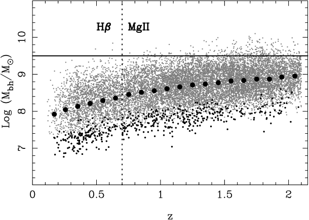
Figure 1: Virial black-hole mass estimate versus redshift for our full SDSS quasar sample. Broad-line quasars (FWHM$\,\geq 2000$ km s^-1) are shown as grey symbols, while narrow-line objects (FWHM$<2000$ km s^-1) are shown as black symbols. The mean black-hole masses within $\Delta z=0.1$ bins are shown as filled circles (standard errors are smaller than the symbols except for lowest redshift bin). The vertical dotted line highlights the switch from using the $H\beta$-based to the MgII-based virial mass estimator at $z=0.7$. The horizontal solid line marks a black-hole mass of $3\times 10^{9}\hbox{$\rm\thinspace M_{\odot}$}$, the maximum mass observed at low redshift (see text for discussion).

The recent publication of the SDSS first data release has provided publically available, fully calibrated, optical spectra of $\geq 17000$ quasars in the redshift interval $0.08<z<2.3$. The flux calibration, long wavelength coverage (3800 Å$<\lambda<\,$9200 Å) and good spectral resolution ($1.4$ Å/pix) of the SDSS spectra make them ideal for use in virial black-hole mass estimates. In this paper we study the black-hole mass distribution of quasars in the redshift range $0.1<z<2.1$ by utilizing continuum and emission-line fits to SDSS quasar spectra, together with calibrations of the virial mass estimators for $H\beta$ and MgII based on those derived by McLure & Jarvis (2002). Via cross-calibration with low-redshift AGN with actual reverberation mapping black-hole mass estimates (Kaspi et al. 2000), it is known that the scatter in the virial mass estimators based on both the $H\beta$ and MgII emission lines is a factor of 2.5 (see McLure & Jarvis 2002; appendix) and, given the potential uncertainties, it is probably unwise to trust individual virial black-hole mass estimates to within a factor of $\simeq 3$. However, because there is no systematic off-set between the virial estimators and the reverberation mapping results, the virial mass estimators are expected to produce statistically accurate results when applied to large samples such as the SDSS.

The structure of the paper is as follows. In Section 2 we described the criteria used for selecting our sample from the SDSS Quasar Catalogue II of Schneider et al. (2003). In Section 3 the basic distribution of the SDSS quasar black-hole masses as a function of redshift is presented. This new information is then used to address important questions regarding the virial black-hole mass estimator and the the accretion rate of luminous quasars. Firstly, a recent study by Netzer (2003) based on the Civ and H$\beta$ virial mass estimators has suggested that many luminous quasars at $z\,\mbox{{\raisebox{-1.72218pt}{$\stackrel{{\scriptstyle>}}{{{\scriptstyle\sim}}}$}}}\,2$ may harbour central black holes with masses in excess of $10^{10}\hbox{$\rm\thinspace M_{\odot}$}$. As highlighted by Netzer (2003), since galaxies with suitably large velocity dispersions ($\sigma\,\mbox{{\raisebox{-1.72218pt}{$\stackrel{{\scriptstyle>}}{{{\scriptstyle\sim}}}$}}}\,600$ km s^-1) are not observed at low redshift, this result raises questions about either the reliability of the virial mass estimator, or the form of the bulge:black-hole mass relation, at high redshift. We re-address this question using our new SDSS quasar black-hole mass estimates based on the MgII calibration of the virial mass estimator.

Secondly, recent studies have shown that at low-redshift ($z\leq 0.5$), luminous broad-line quasars are accreting below the Eddington limit (Floyd et al. 2003; Dunlop et al. 2003; McLeod & McLeod 2001). However, it has been suggested (eg. Mathur 2000) that narrow-line Seyfert galaxies (NLS1) are the low-redshift analogs of the early evolution of luminous quasars, where the central black hole is still in an exponential growth phase, accreting beyond the Eddington limit. Consequently, if NLS1 are the low-redshift analogs of the early evolution of luminous quasars, then at high redshift we might expect to see luminous quasars accreting above the Eddington limit. Using the black-hole mass and bolometric luminosity estimates for our SDSS sample, we investigate whether the Eddington luminosity is still a physically relevant limit to quasar accretion rates at $z\leq 2$.

In Section 4 we re-investigate the form of the local black-hole mass function within the context of the latest results on the $M_{bh}~{}-~{}L_{bulge}$ and $M_{bh}~{}-~{}\sigma$ correlations. In Section 5 this information is combined with the new SDSS quasar black-hole masses and the 2dF quasar luminosity function to estimate the activation fraction of $z\simeq 2$ black holes as a function of mass, and deduce lower limits on the lifetimes of the most luminous quasars. In Section 6 we summarize our main results and conclusions. Full details of the calibration of the virial black-hole mass estimators and the emission-line modelling of the SDSS quasar spectra are provided in the Appendix. Unless otherwise stated all calculations assume the following cosmology : $H_{0}~{}=70$ km s^-1Mpc^-1, $\Omega_{m}=0.3$, $\Omega_{\Lambda}=0.7$.

2 The sample

The sample of quasars analysed in this paper is drawn from the SDSS Quasar Catalog II (Schneider et al. 2003). This catalog is based on the SDSS first data release, and features 16713 quasars with $M_{i}(AB)<-22$ in the redshift interval $0.08~{}<~{}z~{}<~{}5.41$. The first stage in constructing our sample was to select all objects from the Schneider et al. catalog in the redshift range $0.08~{}<~{}z~{}<~{}2.1$, with the upper redshift limit imposed to ensure sufficient wavelength coverage to reliably determine the MgII emission-line widths. The resulting list of 14181 quasars was then passed through the emission-line modelling software described in the Appendix.

The final sample used in the analysis consists of 12698 quasars, or 90% of the $z<2.1$ quasars in the Schneider et al. catalogue. The remaining 10% of objects were excluded for having unreliable modelling results due to low signal-to-noise, particularly weak emission lines or having been affected by artifacts in the spectra. In conclusion, although the SDSS Quasar Catalog II is not statistically complete (Schneider et al. 2003), our final sample of 12698 quasars is clearly representative of optically luminous quasars in the redshift interval $0.1<z<2.1$.

3 The evolution of quasar black-hole masses

In Fig 1 we show the distribution of virial black-hole mass estimates versus redshift for our full SDSS quasar sample. Broad-line quasars (either H$\beta$ or MgII emission line with FWHM$\,\geq 2000$ km s^-1) are shown as grey symbols and narrow-line objects (FWHM$<2000$ km s^-1) are shown as black symbols. The mean black-hole masses within $\Delta z=0.1$ bins are shown as filled circles, and the vertical dotted line at $z=0.7$ marks the transition between the use of the $H\beta$ and MgII based virial estimators. There can be seen to be a smooth transition between the two virial mass calibrations, and more details concerning the quality of the agreement between the $H\beta$ and MgII based virial estimators are provided in the Appendix. Finally, the solid horizontal line is at a black-hole mass of $3\times 10^{9}\hbox{$\rm\thinspace M_{\odot}$}$, which is representative of the maximum mass which has been dynamically measured within the local galaxy population (Ford et al. 1994; Tadhunter et al. 2003).

3.1 Black-hole mass as a function of redshift

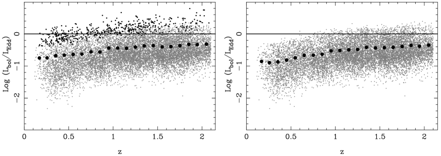
Figure 2: Panel A shows bolometric luminosity as a fraction of the Eddington limit versus redshift for the full sample. The grey symbols are broad-line quasars (FWHM$\,\geq 2000$ km s^-1) and the black symbols are narrow-line objects (FWHM$<2000$ km s^-1). The mean values of $L_{bol}/L_{Edd}$ within $\Delta z=0.1$ bins are shown as filled circles. The solid horizontal line marks the Eddington limit. Panel B is identical to panel A except that only the broad-line quasars have been plotted.

The mean black-hole mass can be seen to increase as a function of redshift, rising from $\simeq 10^{8}\hbox{$\rm\thinspace M_{\odot}$}$ at $z\simeq 0.2$ to $\simeq 10^{9}\hbox{$\rm\thinspace M_{\odot}$}$ at $z\simeq 2.0$. However, this is entirely as expected due to a combination of the effective flux-limit of the sample and the rôle of the quasar continuum luminosity within the virial mass estimator. In the event that the mean FWHM remains approximately constant with redshift, the mean virial black-hole mass estimate is required to increase as $<\lambda L_{\lambda}>^{0.6}$ by construction (Eqn A6 & Eqn A7). The increase in mean black-hole mass with redshift seen in Fig 1 is entirely consistent with this effect.

3.2 Evidence for a limiting black-hole mass

Amongst the sample of local galaxies for which the central black-hole mass has been measured via gas or stellar dynamics, the most massive black holes which have been found to date are in M87 (Ford et al. 1994) and Cyg A (Tadhunter et al. 2003), both with $M_{bh}\simeq 3\times 10^{9}\hbox{$\rm\thinspace M_{\odot}$}$.

Given the relatively small cosmological volume from which this sample of local galaxies is drawn, it is of interest to investigate whether $\simeq~{}3\times~{}10^{9}~{}\hbox{$\rm\thinspace M_{\odot}$}$ represents a genuine limiting mass. Furthermore, the $M_{bh}-\sigma$ and $M_{bh}-L_{bulge}$ correlations, defined by the local galaxies with dynamical black-hole mass measurements, make definite predictions for what the maximum black-hole mass is likely to be. For example, the distribution of stellar-velocity dispersions for early-type galaxies from the SDSS (Bernardi et al. 2003; Seth et al. 2003) show that velocity dispersions of $\stackrel{{\scriptstyle>}}{{{\scriptstyle\sim}}}$ 400 km s^-1 are exceptionally rare among the local galaxy population. Combined with the latest determination of the $M_{bh}-\sigma$ relation (Tremaine et al. 2002), this implies a limiting black-hole mass of $\simeq 2\times 10^{9}\hbox{$\rm\thinspace M_{\odot}$}$, in excellent agreement with the largest black-hole masses measured to date. Consequently, if the virial black-hole mass estimator predicts that a large population of luminous quasars at high redshift harbour black holes with masses $\geq 10^{10}\hbox{$\rm\thinspace M_{\odot}$}$, the implied velocity dispersions of $\sigma\simeq 600$ km s^-1 would be in direct conflict with the known properties of early-type galaxies.

This issue was recently addressed by Netzer (2003), who compiled virial black-hole mass estimates (based on $H\beta$ and Civ emission-line widths) for a heterogeneous sample of 724 quasars in the redshift interval $0<z<3.5$. The results of this study indicated that a significant number of luminous ($\lambda L_{1350}\geq 10^{46.5}$ergs s^-1) quasars are powered by black holes with masses $\mbox{{\raisebox{-1.72218pt}{$\stackrel{{\scriptstyle>}}{{{\scriptstyle\sim}}}$}}}10^{10}\hbox{$\rm\thinspace M_{\odot}$}$. Consequently, Netzer (2003) concluded that either the virial mass estimator (principally the $R_{BLR}-\lambda L_{\lambda}$ correlation) was invalid at $z\,\mbox{{\raisebox{-1.72218pt}{$\stackrel{{\scriptstyle>}}{{{\scriptstyle\sim}}}$}}}\,2$ or, alternatively, that the relationship between black-hole and bulge mass has a different form at high redshift, presumably because the quasar hosts are still in the process of forming.

However, the new results presented here for the SDSS quasars do not appear to support this conclusion. It can be seen from Fig 1 that the upper envelope of black-hole masses for the SDSS quasars is fully consistent with a maximum of $\simeq 3\times 10^{9}\hbox{$\rm\thinspace M_{\odot}$}$, with a negligible number of quasars exceeding this limit at $z\leq 1.5$. At the high-redshift end of the sample ($1.5<z<2.1$) there are only a small number of quasars with virial black-hole mass estimates $\geq 3\times 10^{9}\hbox{$\rm\thinspace M_{\odot}$}$, less than 5% of the SDSS quasars with $z\geq 1.5$, and only two objects are found to have virial black-hole mass estimates in excess of $10^{10}\hbox{$\rm\thinspace M_{\odot}$}$. When the level of scatter associated with the virial mass estimator ($\simeq 0.4$ dex) is taken into account, it is clear that there is no conflict between the SDSS quasar black-hole masses and either the locally observed maximum black-hole mass or, perhaps more significantly, the maximum black-hole mass predicted from combining the stellar-velocity dispersion distribution of early-type galaxies (Bernardi et al. 2003) with the $M_{bh}-\sigma$ relation.

The reason for the discrepancy between the new results presented here and those of Netzer (2003), hereafter N03, is not entirely clear. The distribution of black-hole mass as a function of redshift determined by N03 shows an upper limit consistent with $M_{bh}\simeq 10^{10}\hbox{$\rm\thinspace M_{\odot}$}$, with a small number of objects with estimated masses exceeding this limit. In contrast, the results for the SDSS quasars presented in Fig 1 are consistent with a limit of $\simeq 3\times 10^{9}\hbox{$\rm\thinspace M_{\odot}$}$, a difference of 0.5 dex. The discrepancy cannot be due to the use of different calibrations of the $R_{BLR}-\lambda L_{\lambda}$ correlation. If fact, if our virial mass estimator is adjusted to the same $R_{BLR}-\lambda L_{\lambda}$ slope ($\lambda L_{\lambda}^{0.58}$) and the same geometric normalization (N03 adopt $f=\sqrt{3}/2$, we adopt $f=1$, see Eqn A1) our black-hole mass estimates for the most luminous SDSS quasars are actually reduced by $\simeq 0.2$ dex. Presumably the cause of the discrepancy must therefore lie either in the different methods used to determine the quasar continuum luminosities, or N03’s use of Civ as a proxy for $H\beta$ instead of the MgII FWHM measurements adopted here. In this context we note that Vestergaard (2004) recently found evidence for a similar limiting black-hole mass to that found here, using a smaller sample of $2\,\mbox{{\raisebox{-1.72218pt}{$\stackrel{{\scriptstyle<}}{{{\scriptstyle\sim}}}$}}}\,z\,\mbox{{\raisebox{-1.72218pt}{$\stackrel{{\scriptstyle<}}{{{\scriptstyle\sim}}}$}}}\,4$ quasars and the Civ-based virial mass estimator.

In conclusion, based on the $H\beta$ and MgII virial black-hole mass estimates for $>12000$ SDSS quasars presented here, we find no evidence that $z\leq 2$ quasars harbour central black-holes with masses in excess of the maximum of $\simeq 3\times 10^{9}\hbox{$\rm\thinspace M_{\odot}$}$ observed in the local Universe. This consistency between the most massive black-holes at $z\simeq 2$ and the most massive black-holes at $z\simeq 0$ is important given that it is known from low-redshift studies that the host galaxies of these $z\simeq 2$ quasars must be, or at least evolve into, massive early-type galaxies (Dunlop et al. 2003; McLure & Dunlop 2002; McLeod & McLeod 2001). Reassuringly, the black-hole mass distribution of the SDSS quasars presented here is entirely consistent with their host galaxies having similar properties to those of low-redshift early-types; i.e. $\sigma\,\mbox{{\raisebox{-1.72218pt}{$\stackrel{{\scriptstyle<}}{{{\scriptstyle\sim}}}$}}}\,400$ km s^-1 and $L\,\mbox{{\raisebox{-1.72218pt}{$\stackrel{{\scriptstyle<}}{{{\scriptstyle\sim}}}$}}}\,10\,L^{\star}$.

3.3 Quasar accretion rates

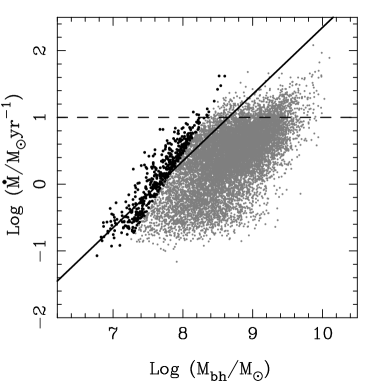
Figure 3: The distribution of the full SDSS sample on the accretion rate $-$ black-hole mass plane. The grey symbols are broad-line quasars (FWHM$\,\geq 2000$ km s^-1) and the black symbols are narrow-line objects (FWHM$<2000$ km s^-1). The solid line shows the location of the Eddington limit ($L_{bol}=L_{Edd}$), while the dashed line highlights an accretion rate of ten solar masses per year, below which 94% of the sample lie.

In panel A of Fig 2 we plot the distribution of quasar Eddington ratios ($L_{bol}/L_{Edd}$) as a function of redshift for the full sample (narrow + broad-line objects). The mean $L_{bol}/L_{Edd}$ values within $\Delta z=0.1$ bins are shown as the filled circles, with the solid horizontal line highlighting the Eddington limit ($L_{bol}/L_{Edd}=1$). Panel B is identical to panel A except that only the broad-line objects are plotted. Several features of the distribution of the SDSS quasars on the $L_{bol}/L_{Edd}-z$ plane are worthy of individual comment and are discussed in turn below.

In common with the distribution of black-hole masses, it can be seen that the mean Eddington ratio of the SDSS quasars increases with redshift, rising from $L_{bol}\simeq 0.15L_{Edd}$ at $z\simeq 0.2$ to $L_{bol}\simeq 0.5L_{Edd}$ at $z\simeq 2.0$ (details of how bolometric luminosities have been estimated from the quasar continuum luminosities are provided in the Appendix). However, due to the fact that the Eddington luminosity is directly proportional to the estimated black-hole mass, the mean Eddington ratio is required to scale as $L_{bol}/L_{Edd}\propto L_{bol}^{\sim 0.4}$ in the event that the mean FWHM is approximately constant with redshift. The increase in the mean Eddington ratio with redshift seen in Fig 2 is entirely consistent with this expectation.

The distribution of Eddington ratios displayed by the SDSS quasars clearly shows that assuming that all luminous quasars are accreting at their Eddington limit is a poor approximation. This result is important because it is often assumed that optically luminous quasars are accreting at their Eddington limit within models of quasar evolution. In fact, our results show that a constant accretion rate of $\simeq 0.3\rightarrow 0.4L_{Edd}$ is a much better approximation than using the Eddington luminosity.

In panel A of Fig 2 it can be seen that the majority of the narrow-line objects (black symbols) are estimated to be accreting at super-Eddington rates. This result is in agreement with numerous studies of low-redshift narrow-line Seyfert 1 galaxies (NLS1) which, in the most widely accepted model, are thought to be examples of low black-hole mass/high accretion rate AGN. However, it is also important to remember that the narrow-line portion of the SDSS quasar sample is likely to be an admixture of genuine narrow-line objects (i.e. low black-hole mass/high accretion rate) and intrinsically broad-line quasars which appear as narrow-line objects simply because they are viewed close to pole-on. Indeed, as discussed in the appendix, if there is any significant disk-component to the FWHM of the broad emission lines then some level of contamination by pole-on sources is inevitable. Within this context it is noteworthy that we do not see any trend for an increase in the numbers of narrow-line objects with redshift, as might be expected under the hypothesis that NLS1s are the low-redshift analogs of the early evolutionary stages of luminous broad-line quasars (eg. Mathur 2000). On the contrary, the fraction of narrow-line objects in our SDSS sample decreases from $\simeq 10\%$ at $z\simeq 0.2$ to only $\simeq 1\%$ at $z\simeq 2$ (see Fig 1). In fact, this trend is at least qualitatively consistent with the predictions of a simplified model of the BLR which depends on both orientation and luminosity. Firstly, if it is assumed that all quasars are intrinsically broad-line objects, and that the BLR has a flattened geometry, then narrow-line objects are simply those which are viewed close to pole-on ($\leq 15^{\circ}$). In a flux-limited sample the proportional of narrow-line objects is then predicted to fall with redshift if the opening angle of the obscuring torus is dependent on the AGN luminosity; i.e $\theta\propto L^{0.5}$ (the so-called “receding torus” model e.g. Simpson 1998). In this simplified scheme the redshift evolution of the narrow-line fraction seen in Fig 1 is roughly consistent with a receding torus model with a half-opening angle of $\simeq 45^{\circ}$ at the low-redshift/luminosity end of the SDSS sample, rising to $\simeq 80^{\circ}$ at the high-redshift/luminosity end.

It can be seen from panel B of Fig 2 that at redshifts $1<z<2$ the upper envelope of the Eddington ratios for the broad-line quasars is virtually flat at $L_{bol}/L_{Edd}\simeq 1$. Indeed, the fact that we do not see significant numbers of quasars which are accreting at greater than the Eddington limit, with virtually none accreting at $\geq 2L_{Edd}$, can be taken as strong evidence that the Eddington limit is a physically meaningful upper limit to the accretion rate in broad-line quasars, at least at $z\,\mbox{{\raisebox{-1.72218pt}{$\stackrel{{\scriptstyle<}}{{{\scriptstyle\sim}}}$}}}\,2\,$.

In Fig 3 we show the distribution of the SDSS quasars on the accretion rate $-$ black-hole mass plane, where the accretion rates have been calculated assuming a canonical mass-to-energy conversion efficiency of $\epsilon=0.1$. The solid line in Fig 3 shows the location of the Eddington limit ($L_{bol}=L_{Edd}$), while the dashed line highlights an accretion rate of ten solar masses per year. It can immediately be seen from Fig 3 that the vast majority (94%) of the SDSS quasars are accreting material at rates of $\mbox{\,$\rm M_{\odot}$}~{}<~{}\hbox{$\dot{M}$}~{}<~{}10\mbox{\,$\rm M_{\odot}$}$ per year. However, perhaps the most striking feature of Fig 3 is the near total lack of quasars with black-hole masses of $M_{bh}>10^{9}\hbox{$\rm\thinspace M_{\odot}$}$ and accretion rates close to the Eddington limit. This feature must be regarded as significant because it is extremely unlikely that large numbers of such objects are missing from the SDSS quasar sample. We note here that this situation is at least qualitatively consistent with models of black-hole growth in which the exponential, Eddington-limited, growth of the black-hole is terminated by a physical limit to the amount of material which can be supplied for accretion (eg. Archibald et al. 2002; Granato et al. 2003, 2001). In models of this type, following the end of the exponential-growth phase the black hole is free to remain active as a luminous quasar for $\simeq 10^{8}$ years, accreting below the Eddington limit, without leading to the production of large numbers of black holes with masses $>10^{10}\hbox{$\rm\thinspace M_{\odot}$}$ which are not observed locally. This type of scenario is also consistent with the results shown in Fig 1 & Fig 2, and is discussed in more detail in Section 5.

4 The local mass function of dormant black holes

Figure 4: Two independent estimates of the redshift zero dormant black-hole mass function for early-type galaxies. The solid line is a transformation of the $K-$band early-type galaxy luminosity function of Kochanek et al. (2001) using the $M_{bh}-L_{bulge}$ correlation of McLure & Dunlop (2002). The dashed line is a transformation of the SDSS early-type galaxy stellar-velocity dispersion function of Seth et al. (2003) using the Tremaine et al. (2002) fit to the $M_{bh}-\sigma$ correlation.

Following the discovery that supermassive black holes appear to be ubiquitous at the centres of massive local galaxies, it has been of interest to use this information to estimate the mass function of dormant black holes in the local Universe. From a theoretical perspective it was shown by Soltan (1982) that the local mass density of dormant black holes could be calculated from the total radiated energy of optical quasars, which in turn can be calculated from the quasar source-count distribution. Traditionally such estimates predict local black-hole mass densities a factor of a few lower (Soltan 1982; Chokshi & Turner 1992; Yu & Tremaine 2002) than those estimated from the X-ray background (eg. Fabian & Iwasawa 1999), suggesting that the dominant fraction of the quasar population is optically obscured. Given that a principal objective of quasar evolution models is to simultaneously explain the evolution of both the quasar luminosity and black-hole mass functions, it is clearly important to have a robust measurement of the form of the local mass function of dormant black holes.

Previous estimates of the local black-hole mass function in the literature have relied on either the $M_{bh}-L_{bulge}$ correlation to make the transformation from the local galaxy luminosity function (e.g. Salucci et al. 1999), or the correlation between radio luminosity and black-hole mass observed in local early-type galaxies (e.g. Franceschini et al. 1998). More recently, both Yu & Tremaine (2002) and Aller & Richstone (2002) exploited the tight $M_{bh}-\sigma$ correlation to derive an estimate of the local mass density of dormant black holes. While the Yu & Tremaine (2002) calculation was based directly on the SDSS stellar-velocity dispersion function, the Aller & Richstone (2002) calculation used the Faber-Jackson relation (Faber & Jackson 1976) to first estimate the dispersion function from the galaxy luminosity function. Despite this difference in approach, both studies found consistent results for the local black-hole mass density (early+late types) with estimates of $(2.4\pm 0.8)\times 10^{5}\hbox{$\rm\thinspace M_{\odot}$}$Mpc^-3 and $(2.9\pm 0.5)\times 10^{5}\hbox{$\rm\thinspace M_{\odot}$}$Mpc^-3 for Aller & Richstone and Yu & Tremaine respectively ($H_{0}=70$ km s^-1Mpc^-1).

In Section 5 we will proceed to estimate the activation fraction of supermassive black holes at $z\simeq 2$. This calculation requires a knowledge of the actual functional form of the local dormant black-hole mass function, information which is unavailable from the previous studies in the literature. At $z\simeq 2$ we are exclusively interested in the form of high-mass end of the local black-hole mass function, and consequently, in this section we use the $M_{bh}-\sigma$ and $M_{bh}-L_{bulge}$ relations to derive two independent estimates of the local black-hole mass function for early-type galaxies.

4.1 The velocity dispersion estimate

Seth et al. (2003) recently performed a detailed analysis of the stellar-velocity dispersion function of 9000 early-type galaxies drawn from the SDSS. As part of this analysis Seth et al. provide a fitting formula for the dispersion function, similar to a Schechter function in form, which is governed by four free parameters $(\phi_{\star},\sigma_{\star},\alpha,\beta)$. As the starting point for our calculation we adopt the best fit determined by Seth et al. to the observed dispersion function, including measurement errors, which is described by the parameter values (0.002 Mpc^-3, 88 km s^-1, 6.5, 1.8). Secondly, we then apply a change of variables to convert the velocity dispersion function into a black-hole mass function using the latest version of the $M_{bh}-\sigma$ correlation ($M_{bh}\propto\sigma^{4.02\pm 0.32}$) as derived by Tremaine et al. (2002). The final step in the process is to convolve this estimate of the black-hole mass function with a gaussian of $\sigma=0.27$ dex to account for the associated scatter of the $M_{bh}-\sigma$ relation. The estimate of the local black-hole mass function produced via this method is shown as the dashed line in Fig 4.

4.2 The bulge luminosity estimate

Our second approach involves a conversion of the local galaxy luminosity function into an estimate of the local black-hole mass function using the $M_{bh}-L_{bulge}$ correlation. This approach was previously used by Salucci et al. (1999), who derived an estimate of the local black-hole mass function via a two-step process. The first stage was the construction of the local bulge/spheroid mass function from representative optical galaxy luminosity functions, segregated by morphological type, using an appropriate mass-to-light ratio and an estimate for each morphological type of the bulge:total light ratio. The second stage was to then convert the spheroid mass function into the black-hole mass function by convolution with a log gaussian $M_{bh}/M_{bulge}$ distribution, centred on $<M_{bh}/M_{bulge}>=-2.6$ with $\sigma=0.3$ dex. The Salucci et al. (1999) study demonstrated that at the high-mass end ($M_{bh}\geq 10^{8}\hbox{$\rm\thinspace M_{\odot}$}$), the local dormant black-hole mass function should be entirely dominated by the contribution from early-type (E+S0) galaxies.

We are now in a position to re-visit this calculation using improved information on the luminosity function of early-type galaxies and the on form of the black-hole mass - bulge mass relation. For the purposes of our estimate we adopt the 2MASS early-type $K-$band luminosity function of Kochanek et al. (2001). The Kochanek et al. early-type luminosity function is conveniently segregated to included only S0 and elliptical galaxies, making it well matched to the SDSS velocity dispersion function of Seth et al. (2003). Moreover, due to the $K-$band selection, we can be confident that the galaxy luminosities trace the mass of the old stellar spheroid population, which has been shown recently to correlate with central black-hole mass with a comparable scatter to the $M_{bh}-\sigma$ correlation; i.e $\simeq 0.3$ dex (McLure & Dunlop 2002; Erwin et al. 2003; Marconi & Hunt 2003).

Specifically, we adopt the $K-$band luminosity function parameters derived by Kochanek et al. (2001) for their early-type (E+S0) sample: $\alpha=-0.92$, $\phi=0.45\times 10^{-2}h_{100}^{3}$ Mpc^-3 and $M_{K}^{\star}=-23.53+5\log h_{100}$. After conversion of the luminosity function parameters to our adopted cosmology, the value of $M_{K}^{\star}$ was further correct by $\Delta m=-0.2$ to transform from isophotal to total magnitudes (Kochanek et al. 2001). In order to make the transformation from the luminosity function to the black-hole mass function we adopt the best-fit to the $M_{bh}-L_{bulge}$ correlation from McLure & Dunlop (2002), which was determined from a sample of exclusively elliptical galaxies with reliable dynamical black-hole mass measurements. After accounting for the change in cosmology, this relation becomes:

$$\log M_{bh}=1.25(\pm 0.05)\log\frac{L_{K}}{\hbox{$\rm\thinspace L_{\odot}$}}-5.76(\pm 0.53)$$ (1)

where an average colour of $R-K=2.7$ for early-type E/S0 galaxies has been adopted (GISSEL98 models; Bruzual & Charlot 1993), and we have also assumed for this simplified calculation that the $K-$band bulge:total luminosity ratio for both elliptical and S0 galaxies is unity. Following convolution with a gaussian with $\sigma=0.3$ dex to account for the scatter around the $M_{bh}-L_{bulge}$ correlation, the final estimate of the early-type dormant black-hole mass function is shown as the solid line in Fig 4.

4.3 Integrated black-hole mass density

It can be seen from Fig 4 that the two independent estimates of the local early-type dormant black-hole mass function are in good agreement at the high-mass end ($M_{bh}\geq 10^{8}\hbox{$\rm\thinspace M_{\odot}$}$). The turn-over of the velocity-dispersion based estimate at low masses is an artifact of the SDSS velocity dispersion function, which turns over at $\sigma\,\mbox{{\raisebox{-1.72218pt}{$\stackrel{{\scriptstyle<}}{{{\scriptstyle\sim}}}$}}}\,125$ km s^-1 due to the faint magnitude limit of the SDSS early-type sample (Bernardi et al. 2003). Finally, if we integrate our estimate of the local black-hole mass function based on the $K-$band luminosity function, our estimate of the local black-hole mass density in early type galaxies is:

$$\rho_{bh}=(2.8\pm 0.4)\times 10^{5}\mbox{\,$\rm M_{\odot}$}{\rm Mpc}^{-3}$$ (2)

which, considering the potential uncertainties and simplified nature of this calculation, can be seen to be in good agreement with the values determined by both Yu & Tremaine (2002) and Aller & Richstone (2002).

The good agreement between the two estimates of the local dormant black-hole mass function found here is apparently in contrast to one of the findings of Yu & Tremaine (2002), who found that using the $M_{bh}-L_{bulge}$ relation led to a black-hole mass density estimate more than a factor of two greater than their velocity dispersion estimate. Although small differences are introduced by our different choice of $M_{bh}-L_{bulge}$ relation and galaxy luminosity function, we note here that the principal source of this apparent discrepancy is that we have adopted virtually identical levels of scatter in the $M_{bh}-\sigma$ and $M_{bh}-L_{bulge}$ relations ($\simeq 0.3$ dex). In contrast, Yu & Tremaine adopted a scatter of $0.5$ dex in the $M_{bh}-L_{bulge}$ relation, based on the fit to $B-$band data by Kormendy & Gebhardt (2001). If the Yu & Tremaine $M_{bh}-L_{bulge}$ density estimate is adjusted to reflect a scatter of $\simeq 0.3$ dex then their two density estimates become consistent, differing by less than 50%. Although the relative levels of scatter associated with the $M_{bh}-\sigma$ and $M_{bh}-L_{bulge}$ relations is currently a question of some debate, our choice of adopting a low scatter of $\simeq 0.3$ dex in the $M_{bh}-L_{bulge}$ relation is justified, especially for early-types, by the recent results of several detailed studies (McLure & Dunlop 2002; Erwin et al. 2003; Marconi & Hunt 2003).

5 Constraining the activation fraction of supermassive black holes

Figure 5: Each panel shows the distribution of absolute $B-$band magnitude for the 1069 quasars from our SDSS sample in the redshift interval $1.90~{}<~{}z~{}<~{}2.1$. The black histograms show the distribution of sub-sets of these quasars whose black-holes are more massive than the thresholds shown in the top-left corner of each panel.

Although the completeness of the SDSS Quasar Catalog II has not been fully quantified (Schneider et al. 2003), there is no obvious reason to suspect that the SDSS quasars are not at least representative of luminous optical quasars. Therefore, it is possible to use our new SDSS quasar black-hole mass estimates to study the distribution of quasar black-hole masses as a function of luminosity. Furthermore, by using the optical quasar luminosity function to calculate the number density of quasars brighter than a given absolute magnitude, it is then possible to estimate the number density of active black-holes as a function of mass. In this section we perform this calculation using our black-hole mass estimates for the SDSS quasars at $z\simeq 2$.

For the purposes of this calculation we adopt the quasar luminosity function as determined by Boyle et al. (2000) for their combined 2dF+LBQS sample of more than 6000 quasars in the redshift range $0.35<z<2.30$. The Boyle et al. luminosity function is defined in terms of absolute $B-$band magnitudes, so we initially convert the bolometric luminosity estimates for our SDSS quasars into absolute $B-$band magnitudes, using a transformation defined by $>300$ quasars common to both the SDSS and the 2dF 10K quasar catalog (Croom et al. 2001; see Appendix).

In Fig 5 we show the distribution of absolute $B-$band magnitude for 1069 SDSS quasars in the redshift interval $1.90~{}\leq~{}z~{}\leq~{}2.10$. The filled histograms in each panel show the distribution of absolute $B-$band magnitudes for three sub-sets of these objects which have black-hole masses greater than our chosen mass thresholds of $10^{8.5}\hbox{$\rm\thinspace M_{\odot}$},10^{9}\hbox{$\rm\thinspace M_{\odot}$}$  &  $10^{9.5}\hbox{$\rm\thinspace M_{\odot}$}$. The solid line at $M_{B}=-26$ shows the location of the $m_{i}(AB)=19.1$ (Schneider et al. 2003) flux limit of the main SDSS multi-colour quasar selection algorithm at $z=2.1$. Provided that at a given quasar luminosity the SDSS is not significantly biased towards including only the most massive black-holes, the ratio of the filled to un-filled histograms in Fig 5 provides a method for determining lower limits on the number densities of active black holes at $z\simeq 2$.

We perform this calculation in two steps. Firstly, for each of the three mass thresholds we calculate the fraction $f$ of quasars with black-hole masses above the threshold, in three magnitude ranges: $-25<M_{B}<-26$, $-26<M_{B}<-27$ & $-27<M_{B}<-28.3$ (switching to 0.5 magnitude bins makes little difference to the final estimate). The lower limit of $M_{B}=-25$ has been chosen to conservatively ensure that we still have sufficient numbers of quasars in the filled histograms to determine $f$ in each magnitude bin to better than 10% accuracy. Although $M_{B}=-25$ is one magnitude fainter than the SDSS quasar selection algorithm flux limit at $z\simeq 2$, we are making the explicit assumption that the ratio of the filled to un-filled histograms would remain unchanged, even in the event that the SDSS quasar selection was complete to $M_{B}=-25$. The second step in the process is to use the Boyle et al. (2000) quasar luminosity function to calculate the number density of quasars ($\rho_{act}$) in the three magnitude bins at $z=2$. For this calculation we adopt the Boyle et al. polynomial fit to the luminosity function, converting the absolute magnitude limits and number densities to our adopted cosmology. Finally, the estimated number densities of active black-holes for each of the mass thresholds is simply the sum of $f\times\rho_{act}$ over the three magnitude bins.

The estimates of the number densities of active supermassive black holes at $z\simeq 2$ using the above method are shown in panel A of Fig 6, for the three black-hole mass thresholds. Also shown are the $z\simeq 0$ cumulative black-hole mass functions based on our $M_{bh}-L_{bulge}$ and $M_{bh}-\sigma$ estimates from Section 4. This plot indicates that the fraction of present-day black holes which are in place, active, and optically unobscured at $z\simeq 2$ is $\simeq 0.005$ for $M_{bh}\geq 10^{8.5}{\rm M_{\odot}}$, $\simeq 0.02$ for $M_{bh}\geq 10^{9}{\rm M_{\odot}}$, and $\simeq 0.05$ for $M_{bh}\geq 10^{9.5}{\rm M_{\odot}}$.

How should we interpret these ratios? The actual observed number density ratio at a given mass threshold, R, must be a product of three physical ratios, namely:

$$$$R=(n_{z=2}/n_{z=0})\times(t_{Q}/t_{epoch})\times(n_{vis}/n_{obs})$$$$ (3)

where $n_{z=2}$ is the number density of black holes (above the appropriate mass threshold) already in place at $z=2$, $n_{z=0}$ is the corresponding number density at the present day, $t_{Q}$ is the net lifetime of a black hole (above the appropriate mass threshold) in the optically luminous quasar phase, $t_{epoch}$ is the total duration of the luminous quasar epoch, and the ratio $(n_{vis}/n_{obs})$ describes the effect of geometrical obscuration by dusty tori (note the effect of a completely obscured phase is different, and is implicitly taken care of by the definition of $t_{Q}$).

Figure 6: In each panel the solid and dashed lines show the cumulative local dormant black-hole mass functions as derived in Section 4 using the $M_{bh}-L_{bulge}$ and $M_{bh}-\sigma$ relations respectively. In panel A we show the estimated number densities of active supermassive black-holes at $z\simeq 2$ for three mass thresholds ($\geq 10^{8}\mbox{\,$\rm M_{\odot}$},\geq 10^{9}\mbox{\,$\rm M_{\odot}$}\,\&\geq 10^{9.5}\mbox{\,$\rm M_{\odot}$}$). In panel B these number densities have be adjusted to account for a possible relationship between mean quasar lifetime and black-hole mass (see text for discussion). In Panel C the number densities of supermassive black-holes have been boosted by a factor of two to conservatively account for geometric obscuration.

Thus, while at first sight it might appear that panel A in Fig 6 indicates that the fraction of present-day black holes already in place at $z\simeq 2$ is an increasing function of mass, this could equally well reflect a mass-dependence of either net quasar lifetime, or torus opening angle. Some interesting limiting values can, however, be deduced with reasonable confidence. For example, adopting $t_{epoch}=2$ Gyr (corresponding to the redshift range $1.5<z<3.5$, the full width half maximum of the peak in luminous quasar number density - see, e.g. Richstone et al. (1998); Osmer 2003), we can infer a lower limit on the optical quasar lifetime of the most massive black holes $M\geq 10^{9.5}{\rm M_{\odot}}$ of $t_{Q}>1\times 10^{8}$ yr if there are no type II quasars, or $t_{Q}>2\times 10^{8}$ yr if $(n_{vis}/n_{obs})\simeq 0.5$ as found at the bright end of the radio-loud quasar population. Such numbers seem very reasonable, agreeing well with, for example, the recent findings of Yu & Tremaine (2002). The fact that $t_{Q}>1\times 10^{8}$ yr differs spectacularly from, for example, the conclusion reached by Richstone et al. (1998) that $t_{Q}\simeq 1\times 10^{6}$ yr, can be traced to the fact that our inferred quasar black-hole masses are on average larger (because we have not been forced to assume Eddington limited accretion) and the fact our analysis is confined to the very high-mass end of the black-hole mass function.

In fact, as a result of their analysis, Yu & Tremaine (2002) find evidence for a mass dependence of $t_{Q}$ which can largely explain the apparent mass dependence of activity ratio shown in panel A of Fig 6. Specifically, Yu & Tremaine determined that the mean quasar lifetime should be an increasing function of black-hole mass, rising from $3\times 10^{7}$ yr at $10^{8}\hbox{$\rm\thinspace M_{\odot}$}$ to $5\times 10^{8}$ yr at $10^{9.5}\hbox{$\rm\thinspace M_{\odot}$}$. For illustrative purposes, we show in panel B of Fig 6 the effect of correcting the estimated number densities at $z\simeq 2$, using the appropriate values of $t_{Q}$ as a function of mass (from Fig. 5 of Yu & Tremaine) and again adopting $t_{epoch}=2$ Gyr. This has the effect of removing all significant mass dependence, and raises the apparent black-hole activation ratio to $\geq 0.2$ for all three mass thresholds. Applying a conservative correction of $\simeq 2$ for geometric obscuration raises this ratio to $\geq 0.4$ (see panel C of Fig 6). Given that our $z\simeq 2$ census is undoubtedly incomplete (being confined to the very luminous end of the quasar population) this lower limit is sufficiently close to unity to imply that the majority of supermassive black holes are in place by $z\simeq 2$, and to leave little, if any, room for an additional substantial population of completely obscured growing black holes at the high-mass end. This finding is in accord with the conclusions of Yu & Tremaine (2002), and Fabian (2003) that the apparently substantial obscured population of AGN required to explain the X-ray background is to be found at lower black hole masses than those probed by the present study.

Finally, we note that values of quasar lifetime ($t_{Q}$) as large as a significant fraction of a Gyr as discussed above, have often been rejected as unfeasible for the most massive black holes $M>10^{9}\hbox{$\rm\thinspace M_{\odot}$}$. This is because, if accretion is assumed to proceed at, or close to, the Eddington limit, extreme black hole masses $M>10^{10}\hbox{$\rm\thinspace M_{\odot}$}$ will then be produced in only $1\times 10^{8}$ yr, and as discussed in Section 3.2 we find no evidence for any significant population of such extreme-mass black holes within the SDSS quasar sample. However, the lack of such extreme objects can be reconciled with our inferred lower limit on quasar lifetime $t_{Q}>2\times 10^{8}$ yr by revisiting the results shown in Fig 3. Here it can be seen that continued Eddington-limited exponential growth towards $M\simeq 10^{10}\hbox{$\rm\thinspace M_{\odot}$}$ requires mass accretion rates which rapidly approach $100{\rm M_{\odot}yr^{-1}}$. In contrast, allowing for the known scatter in the calculation of bolometric luminosities (Elvis et al. 1994), Fig 3 provides good evidence that the most massive black holes are not accreting matter at a rate significantly in excess of $10{\rm M_{\odot}yr^{-1}}$. Clearly, a $10^{9}\hbox{$\rm\thinspace M_{\odot}$}$ black hole can continue to accrete matter at this rate, and produce bright quasar light for a substantial fraction of a Gyr without producing a final black-hole mass in excess of a few times $10^{9}\hbox{$\rm\thinspace M_{\odot}$}$.

In conclusion, our results imply that the majority of the most massive black-holes are in place by $z\simeq 2$ and that the most massive black holes accrete the bulk of their final mass (i.e. as they grow from $\simeq 10^{8.5}\hbox{$\rm\thinspace M_{\odot}$}$ to $\simeq 10^{9.5}\hbox{$\rm\thinspace M_{\odot}$}$) as optically luminous quasars, at a growth rate limited not by the Eddington limit but by some other physical limit on fuel supply which prevents accretion rates significantly in excess of $10{\rm M_{\odot}yr^{-1}}$. Such a physical limit on black-hole fuel supply might be imposed by accretion disc physics (e.g. the calculations of Burkert & Silk (2001) indicate that accretion disc viscosity can be expected to limit the mass consumption rate of a supermassive black-hole at the centre of a forming spheroid to $\simeq 2-20{\rm M_{\odot}yr^{-1}}$) or by the physics of galaxy formation (e.g. Archibald et al. 2002; Granato et al. 2001, 2003). In addition, one might speculate that the apparent lack of a substantial population of highly obscured supermassive black holes may be a consequence of this sub-Eddington accretion, as compared to the Eddington-limited accretion more likely to be experienced by lower mass objects (Fabian 2003).

6 Conclusions

Virial black-hole mass estimates have been calculated for a sample of 12698 quasars in the redshift interval $0.1<z<2.1$ drawn from the SDSS Quasar Catalogue II (Schneider et al. 2003). The distribution of the quasar black-hole masses as a function of redshift has been presented and compared with the masses of dormant black-holes observed in the local Universe. In addition, the quasar host-galaxy properties implied from an application of the locally observed relationship between black-hole and bulge mass have been compared with the known properties of local early-type galaxies. By combining the black-hole mass estimates with the quasar bolometric luminosities the distribution of quasar accretion rates have been investigated. Furthermore, in combination with the optical quasar luminosity function, the new SDSS black-hole mass estimates have been used to estimate the number density of active black-holes at $z\simeq 2$ as a function of mass. Finally, the activation fraction of black holes at $z\simeq 2$ has been estimated by comparing the estimated number density of active black holes with the local dormant black-hole mass function. The main conclusions of this study can be summarized as follows:

1. The virial black-hole mass estimates of the SDSS quasars are entirely consistent with an upper boundary of $\sim 3\times 10^{9}\hbox{$\rm\thinspace M_{\odot}$}$. This limit is consistent with both the most massive black-holes measured dynamically in the local Universe, and the expected black-hole mass limit based on the known properties of early-type galaxies and the locally observed correlation between bulge and black-hole mass. Consequently, using the MgII-based virial mass estimator, no evidence is found for a conflict between quasar black-hole masses in the redshift range $0.1<z<2.1$ and the contemporary, or ultimate properties of their host-galaxy population.

2. The estimated Eddington ratios of the SDSS quasars show only a small level of evolution over the redshift range $0.0<z<2.1$, rising from $L_{bol}\simeq 0.15L_{Edd}$ at $z\simeq 0.2$ to $L_{bol}\simeq 0.5L_{Edd}$ at $z\simeq 2.0$. Although the most luminous broad-line SDSS quasars are accreting at rates up to the Eddington limit by $z\simeq 1$, there does not appear to be a significant change in accretion rates in the redshift range $1<z<2$, with the most luminous broad-line SDSS quasars in the current sample still accreting within a factor of $\simeq 2$ of the Eddington limit at $z\simeq 2$. Consequently, it appears from these results that the Eddington limit is still a relevant physical boundary to the accretion rate of luminous broad-line quasars, at least at $z\,\mbox{{\raisebox{-1.72218pt}{$\stackrel{{\scriptstyle<}}{{{\scriptstyle\sim}}}$}}}\,2$.

3. Using the latest determinations of the galaxy luminosity and stellar-velocity dispersion functions, estimates of the local dormant black-hole mass function for early-type galaxies using the $M_{bh}-\sigma$ and $M_{bh}-L_{bulge}$ relations are shown to be consistent at the high-mass end ($M_{bh}>10^{8}\hbox{$\rm\thinspace M_{\odot}$}$). The agreement between the two methods is found to be dependent on the adoption of similar levels of association scatter ($\simeq 0.3$ dex) in both correlations. Our best estimate of the total mass density of dormant black holes within the local early-type galaxy population is $\rho_{bh}=(2.8\pm 0.4)\times 10^{5}\mbox{\,$\rm M_{\odot}$}{\rm Mpc}^{-3}$.

4. The activation fraction of supermassive black-holes at $z\simeq 2$ is apparently an increasing function of mass, with an activation rate of $f\simeq 0.005$ at $M_{bh}\simeq 10^{8.5}\hbox{$\rm\thinspace M_{\odot}$}$ rising to $f\simeq 0.05$ at $M_{bh}\simeq 10^{9.5}\hbox{$\rm\thinspace M_{\odot}$}$. However, it is shown that this result is consistent with theoretical work which predicts quasar lifetimes to be an increasing function of black-hole mass. Correcting for this expectation we find that the shape of the active black-hole mass function at $z\simeq 2$ is consistent with that of the local dormant black-hole mass function, with a normalization a factor of $\simeq 5$ lower. Making a conservative correction of a factor of two to account for geometric obscuration, the direct implication of this result is that the fraction of black-holes with mass $\geq 10^{8.5}\hbox{$\rm\thinspace M_{\odot}$}$ which are in place and active at $z\simeq 2$ is $\geq 0.4$.

5. A fairly robust limit on the lifetime of quasars with black-hole masses $\geq 10^{9.5}\hbox{$\rm\thinspace M_{\odot}$}$ is found to be $t_{Q}>2\times 10^{8}$ years. Black holes of this mass appear to be prevented from growing to masses $>10^{10}\hbox{$\rm\thinspace M_{\odot}$}$ by some physical mechanism, other than the Eddington limit, which prevents accretion at rates $\mbox{{\raisebox{-1.72218pt}{$\stackrel{{\scriptstyle>}}{{{\scriptstyle\sim}}}$}}}\,10\,\hbox{$\rm\thinspace M_{\odot}$}$ per year.

7 acknowledgments

RJM acknowledges the award of a PPARC PDRA. JSD acknowledges the enhanced research time provided by the award of a PPARC Senior Fellowship. The authors acknowledge Matt Jarvis for useful discussions. Funding for the Sloan Digital Sky Survey (SDSS) has been provided by the Alfred P. Sloan Foundation, the Participating Institutions, the National Aeronautics and Space Administration, the National Science Foundation, the U.S. Department of Energy, the Japanese Monbukagakusho, and the Max Planck Society. The SDSS Web site is http://www.sdss.org/. The SDSS is managed by the Astrophysical Research Consortium (ARC) for the Participating Institutions. The Participating Institutions are The University of Chicago, Fermilab, the Institute for Advanced Study, the Japan Participation Group, The Johns Hopkins University, Los Alamos National Laboratory, the Max-Planck-Institute for Astronomy (MPIA), the Max-Planck-Institute for Astrophysics (MPA), New Mexico State University, University of Pittsburgh, Princeton University, the United States Naval Observatory, and the University of Washington.

Appendix A The virial black-hole mass estimate

The assumption that certain broad-emission lines present in the spectra of Type 1 quasars trace the virialized velocity field of the broad-line region (BLR) leads to the so-called virial black-hole mass estimate:

$$M_{bh}=G^{-1}R_{BLR}V_{BLR}^{2}$$ (4)

where $R_{BLR}$ is the BLR radius and $V_{BLR}$ is the Keplerian velocity of the line-emitting gas. Recent evidence in the literature which supports the basic assumption of virialized motions in the BLR has been previously discussed in introduction. In this Appendix we describe the derivation of the final versions of the virial mass estimators, based on both the $H\beta$ and MgII emission lines, used to estimate the SDSS quasar black-hole masses. Much of this material has been discussed previously by McLure & Jarvis (2002), and the reader is referred to this paper for more details. The material is partly repeated here for completeness, and to highlight a change in the adopted calibration of the $R_{BLR}-\lambda L_{\lambda}$ relation at 3000 Å which is integral to the MgII based virial black-hole mass estimator.

A.1 Estimating the broad-line region radius

In the absence of reverberation mapping it is necessary to estimate $R_{BLR}$ via the correlation between $R_{BLR}$ and AGN continuum luminosity (Wandel, Peterson & Malkan 1999; Kaspi et al. 2000). In McLure & Jarvis (2002) the best-fitting $R_{BLR}-\lambda L_{\lambda}$ relations were derived at both 3000 Å  and 5100 Å  for the 34 AGN with reverberation mapping estimates of $R_{BLR}$ from Wandel, Peterson & Malkan (1999) and Kaspi et al. (2000). Using the BCES method of Akritas & Bershady (1996) the bisector fits at both wavelengths were as follows:

$$R_{BLR}=(25.2\pm 3.0)\left[\lambda L_{3000}/10^{37}W\right]^{(0.47\pm 0.05)}$$ (5)

$$R_{BLR}=(26.4\pm 4.4)\left[\lambda L_{5100}/10^{37}W\right]^{(0.61\pm 0.10)}$$ (6)

where $R_{BLR}$ is in units of light-days. The sample of 34 AGN with reverberation mapping estimates of $R_{BLR}$ is composed of 17 PG quasars and 17 lower-luminosity Seyfert galaxies spanning the luminosity range $10^{34}$W$<\lambda L_{\lambda}<10^{39}$W. While this luminosity range is fairly representative of the SDSS quasars analysed using the $H\beta$ emission line ($0.1<z<0.5$), it is not representative of the SDSS quasars at $z\geq 0.7$, where we have utilized the MgII emission line to estimate their black-hole masses. Simply as a result of their higher redshifts, these quasars reside exclusively in the luminosity range $10^{37}$W$<\lambda L_{\lambda}<10^{40}$W. Consequently, in order to provide as accurate an estimate of the $R_{BLR}$ for each quasar as possible, it was decided to re-fit the $R_{BLR}-\lambda L_{\lambda}$ relation at 3000 Å  using only those objects from the reverberation mapped AGN sample with $\lambda L_{\lambda}>10^{37}$W. Following McLure & Jarvis (2002) we again adopt the BCES bi-sector fit as our best estimate of the $R_{BLR}-\lambda L_{\lambda}$ relation at 3000 Å , with the following result:

$$R_{BLR}=(18.5\pm 6.6)\left[\lambda L_{3000}/10^{37}W\right]^{(0.62\pm 0.14)}$$ (7)

which is shown along with the previous $R_{BLR}-\lambda L_{3000}$ fit from McLure & Jarvis (2002) in Fig A1. It can be seen from Fig A1 that although the two fits are consistent, the new steeper $R_{BLR}-\lambda L_{3000}$ relation does provide a better fit to the reverberation mapped PG quasars of Kaspi et al. with $L_{\lambda}>10^{37}$W, which are typical of the SDSS quasars at $z\geq 0.7$. Consequently, it is the new steeper form of the $R_{BLR}-\lambda L_{3000}$ relation which is adopted throughout the analysis performed in this paper. The fit to the $R_{BLR}-\lambda L_{5100}$ relation determined by McLure & Jarvis (2002) is adopted unchanged because of the lower luminosity range occupied by the SDSS quasars at $z\leq 0.7$.

Figure 7: The $R_{BLR}-\lambda L_{3000}$ relation for the 34 AGN with reverberation mapping estimates of $R_{BLR}$ from Kaspi et al. (2000). The solid line is the best-fitting BCES bi-sector fit determined for the full sample by McLure & Jarvis (2002); Eqn A2. The dotted line shows the new steeper relation adopted in this paper, which is a fit to those objects with $\lambda L_{\lambda}>10^{37}$W.

A.2 Broad-line region geometry

In Eqn 4 the velocity of the BLR gas is taken as $V_{BLR}=$ $f\times$ FWHM, where FWHM is the full-width half maximum of your chosen broad emission line (either $H\beta$ or MgII in this case) and $f$ is a geometric factor which relates the FWHM to the intrinsic Keplerian velocity of the broad-line gas.

Due to the fact that there is currently no consensus on the geometry of the BLR in radio-quiet quasars it is conventional to set $f=\sqrt{3}/2$ , which is appropriate if the orbits of the BLR gas are randomly orientated. Perhaps the most likely alternative to randomly orientated BLR orbits is the possibility that the geometry of the BLR is flattened or disk-like in nature. In radio-loud quasars, where a rough orientation indicator is available from the radio core-to-lobe ratio, there is good evidence that broad-emission line FWHM show a orientation dependence consistent with a disk-like geometry (e.g. Browne & Wills 1986; Brotherton 1996). Given the similarity between the optical emission-line spectra of radio-loud and radio-quiet quasars, it is perhaps not unreasonable to consider the possibility that the BLR of radio-quiet quasars (which dominate the SDSS sample) are also flattened. As discussed by McLure & Dunlop (2002), in this case:

$$V_{BLR}=FWHM/(2\times\sin i)$$ (8)

where $i$ is the angle between the line-of-sight and the disk axis (i.e. $i=0^{\circ}$ is pole-on). It has been established for radio-loud quasars that the angle to the line-of-sight is consistent with being randomly distributed between $0^{\circ}<i<45^{\circ}$ (Barthel 1989; Willott et al. 2000). Assuming the same situation to be true for radio-quiet quasars, it follows that the mean line-of-sight angle will be $<i>=30^{\circ}$ (averaging over solid angle) implying that $<f>=1$. Consequently, it can be seen that $f=1$ represents a good choice of geometric factor in the case of both random or flattened BLR orbits and is adopted throughout this paper. We note that if the BLR of radio-quiet quasars is flattened, objects which are aligned closer than 15^∘ to the line-of-sight will have their black-hole masses underestimated by a factor of $>4$. However, these objects should only represent a small fraction of the SDSS sample ($\simeq 10\%$ if $i$ is randomly distributed in the range $0^{\circ}<i<45^{\circ}$) and will likely appear as narrow-line objects (FWHM$<2000$ km s^-1), which are not the principal focus of this paper. A discussion of the evidence for the flattened BLR hypothesis provided by the SDSS sample is presented in Section 3.3.

A.3 The virial black-hole mass estimators

Substituting the calibrations of the $R_{BLR}-\lambda L_{\lambda}$ relations into Eqn A1, and making the identification that $V_{BLR}$ = MgII or H$\beta$ FWHM, we arrive at the virial black-hole mass estimators. As in McLure & Jarvis (2002), these virial estimators are then compared to the black-hole masses of the reverberation mapped AGN from the Kaspi et al. sample. By requiring that on average the new virial estimators match the mass estimates derived by Kaspi et al. (2000), using the reverberation mapping values of $R_{BLR}$ and rms FWHM measurements, small off-sets of $-0.05$ dex and $-0.04$ dex are introduced to the MgII and H$\beta$ estimators respectively. Accounting for these off-sets we arrive at the final versions of the virial black-hole mass estimators adopted throughout the analysis in this paper:

$$\frac{M_{bh}}{\mbox{\,$\rm M_{\odot}$}}=3.2\left(\frac{\lambda L_{3000}}{10^{37}{\rm W}}\right)^{0.62}\left(\frac{FWHM(MgII)}{{\rm kms}^{-1}}\right)^{2}$$ (9)

$$\frac{M_{bh}}{\mbox{\,$\rm M_{\odot}$}}=4.7\left(\frac{\lambda L_{5100}}{10^{37}{\rm W}}\right)^{0.61}\left(\frac{FWHM(H\beta)}{{\rm kms}^{-1}}\right)^{2}$$ (10)

where the H$\beta$ based black-hole mass estimator is unchanged from that derived by McLure & Jarvis (2002).

A.4 Comparing the ${\bf H\beta}$ and MgII based estimators

Figure 8: The top panel shows a histogram of the log of the ratio of H$\beta$/MgII FWHM for 1136 objects in the redshift interval $0.5<z<0.8$. The mean log ratio is $-0.004\pm 0.005$, with a dispersion of 0.16 dex. The middle panel shows a histogram of the log of the ratio of $R_{BLR}$ as estimated via the $R_{BLR}-\lambda L_{\lambda}$ relation at 5100 Å  and 3000 Å  respectively. The mean log $R_{BLR}$ ratio is $0.0010\pm 0.0021$, with a dispersion of 0.07 dex. The bottom panel shows a histogram of the log of the ratio of virial black-hole mass estimate based on the $H\beta$ and MgII emission lines and the $R_{BLR}-\lambda L_{\lambda}$ relations at 5100Å  and 3000Å  respectively. The mean log ratio is $0.013\pm 0.010$ with a dispersion of 0.33 dex.

McLure & Jarvis (2002) compared the $H\beta$ and MgII based virial estimators using a sample of 150 quasars drawn from the LBQS (Forster et al. 2001) and MQS samples (Baker et al. 1999) which had spectra covering both emission lines. The result of this comparison showed that $M_{bh}(H\beta)\propto M_{bh}(MgII)^{1.00\pm 0.08}$ with a $1\sigma$ scatter in $\log M_{bh}$ of 0.41 dex. Here we can re-investigate the agreement between the two virial mass estimators more thoroughly using the 1136 SDSS quasars from our sample in the redshift range $0.5<z<0.8$ where it was possible to estimate the black-hole mass using both $H\beta$ and MgII. The results of this comparison are illustrated in Fig A2. The top panel shows the distribution of the ratio of the FWHMs of the $H\beta$ and MgII emission lines. The middle panel shows the distribution of the ratio of broad-line region radius, as estimated via the $R_{BLR}-\lambda L_{\lambda}$ correlations at 5100 Å  and 3000 Å  respectively. The distributions of the FWHM and $R_{BLR}$ ratios shown in the top and middle panels are both centred on unity, with $1\sigma$ scatters of 0.16 dex and 0.07 dex respectively. The bottom panel shows the distribution of the ratio of black-hole mass, as estimated via Eqn A7 and Eqn A6 respectively. The mean log ratio of the black-hole mass estimates is $0.013$ with a $1\sigma$ scatter of 0.33 dex. In conclusion, this comparison demonstrates that the MgII and $H\beta$ based virial mass estimators return the same mass estimates within a factor of $\simeq 2$ on average, and that statistically are entirely interchangeable. This conclusion is re-enforced by the smooth transition between the two estimators at $z\simeq 0.7$ shown in Fig 1.

Appendix B Model fitting

Figure 9: An example of the emission-line fitting process in the $H\beta$ region for an SDSS quasar at z=0.17. The upper plot shows the original spectrum shifted to the rest-frame (thin line) with the best-fitting model over-plotted as the thick line. Also shown in the upper plot is the fitted power-law quasar continuum (dotted line). The lower plot shows the original spectrum after subtraction of the best-fitting quasar continuum and iron-emission template. The thick solid line shows the best-fitting model, while the thin solid line shows the individual emission-line components which comprise the best-fitting model.

Figure 10: An example of the emission-line fitting process in the MgII region for an SDSS quasar at z=0.88. The upper plot shows the original spectrum shifted to the rest-frame (thin line) with the best-fitting model over-plotted as the thick line. Also shown in the upper plot is the fitted power-law quasar continuum (dotted line). The lower plot shows the original spectrum after subtraction of the best-fitting quasar continuum and iron-emission template. The thick solid line shows the best-fitting model, while the thin solid line shows the individual emission-line components which comprise the best-fitting model.

Due to the size of the sample of SDSS quasars analysed here, the fitting of the $H\beta$ and MgII emission lines and the determination of the continuum luminosities at 5100 Å  and 3000 Å  was undertaken in a fully automated fashion. The various stages in the emission-line modelling of both $H\beta$ and MgII are discussed below.

B.1 Continuum and iron-template fitting

In order to reliably measure the line-widths of the $H\beta$ and MgII emission lines it is necessary to subtract the surrounding iron emission. This subtraction process can often be important for fitting the $H\beta$ emission line, but is crucial for fitting the MgII emission line where the wings are usually strongly blended with the surrounding FeII emission. The approach adopted here for dealing with the iron emission is a variant on the technique developed by Boroson & Green (1992), which is based on the fitting of an iron-emission template derived from the spectrum of narrow-line Seyfert galaxy (NLS1) Izw1. As a member of the NLS1 class, Izw1 is ideal for this purpose because it displays extremely strong iron emission around both $H\beta$ and MgII with a FWHM of $\simeq 900$ km s^-1. Consequently, the strength and FWHM of an iron template based on Izw1 can be adjusted to match the iron emission of broad-line quasars where the FWHM of the iron emission is $\geq 2000$ km s^-1. The iron emission templates used in the modelling are taken from two different sources, but are both derived from spectra of Izw1. For the modelling of the $H\beta$ emission line we have used the optical FeII emission template derived by Marziani et al. (2003), which is made freely available by the authors. For the modelling of the MgII emission line we have reconstructed the FeII+FeIII emission template derived by Vestergaard & Wilkes (2001) from the data published within that paper.

The first stage in the modelling process of both the $H\beta$ and MgII emission lines is the simultaneous fitting of the underlying quasar continuum and the iron-emission template, where the quasar continuum is assumed to be a simple power-law ($f_{\nu}\propto\nu^{-\alpha}$). For both emission lines this fitting was performed in two wavelength windows, which conservatively excluded the $H\beta$ and MgII emission regions to avoid biasing the iron-emission fit with the wings of the line emission. For the $H\beta$ emission line the continuum+FeII fitting windows were 4435 Å $\rightarrow$ 4700 Å  and 5100 Å $\rightarrow$5535 Å . The equivalent regions for the MgII emission line where 2100 Å $\rightarrow$ 2675 Å  and 2925 Å $\rightarrow$3090 Å . During the fitting process the normalization and slope of the continuum were left as free parameters, as were the luminosity and FWHM of the iron template. Upon completion of this process the best-fitting continuum+iron combination was subtracted from the spectra, leaving the isolated MgII or $H\beta$+[Oiii] emission lines. The fitting of the MgII and $H\beta$ emission lines then proceeded in slightly different fashions, and are therefore described separately below.

B.2 Fitting the $H\beta$+[Oiii] emission-line complex

The $H\beta$ and [Oiii] emission lines were modelled simultaneously as a combination of four components: broad and narrow $H\beta$ plus narrow components for [Oiii] 4959 Å  and [Oiii] 5007 Å . In order to limit the degrees of freedom involved in the fitting several restrictions were invoked. Firstly, the central wavelengths of the narrow $H\beta$ component and the [Oiii] 4959 Å  component were constrained to lie at their laboratory wavelength offsets with respect to [Oiii] 5007 Å. This meant that there were only two free central wavelengths involved in the fit, that of the broad $H\beta$ component and [Oiii] 5007 Å . Secondly, the FWHM of the narrow $H\beta$ component and the two [Oiii] components were constrained to have the same value. The final restriction imposed was that the FWHM of the narrow components was constrained to be less than 2000 km s^-1.

Four different representations of the line profiles were tried for each object. Firstly, two fits were performed where all the line profiles (broad+narrow $H\beta$ and [Oiii] 4959 & 5007) were first modelled as gaussians and then as lorentzians. Secondly, two further fits were performed where the broad $H\beta$ profile was first modelled as a gaussian, with all the narrow profiles modelled as lorentzians, and then secondly with broad $H\beta$ modelled as a lorentzian with all the narrow profiles modelled as gaussians. The FWHM value used in the virial mass estimates is that of the best-fitting model profile, in terms of $\chi^{2}$, within the line-fitting region (4700 Å $\rightarrow$ 5100 Å ).

B.3 Fitting the MgII emission line

The first stage of the modelling of the MgII emission line involved the fitting of a two-component, broad+narrow profile. This proceeded in similar fashion to the modelling of the $H\beta$ emission line, with both the narrow and broad components first represented as either gaussians or lorentzians. In addition, two further model fits were tried for each object, the first comprising a gaussian broad component and a lorentzian narrow component, and the second a lorentzian broad component and a gaussian narrow component. During this stage of the modelling the central wavelength, FWHM and flux of both the narrow and broad components were treated as free parameters. The only restriction invoked was that the narrow component had a FWHM $\leq 2000$ km s^-1. Both the narrow and broad components were modelled as doublets separated by their laboratory wavelength difference, and all of the emission-line models were fitted within the wavelength range 2700 Å $\rightarrow$ 2900 Å .

Unlike the $H\beta$ emission line, which often displays a clear point of inflection between the narrow and broad components, with MgII it is often unclear whether a significant, separate narrow component is present. To account for this, the MgII emission line of each quasar was also modelled as a single broad lorentzian or gaussian doublet. For the purposes of the virial mass estimates the FWHM of the broad component of the best-fitting two-component model profile was adopted as the best FWHM estimate for each quasar, provided that two criteria were satisfied. Firstly, the $\Delta\chi^{2}$ between the best-fitting two-component and best-fitting single-component models was required to be significant at the $3\sigma$-level, i.e. the extra degrees of freedom in the two-component model had to be justified statistically. Secondly, the equivalent width (EW) of the broad component was required to be greater than two-thirds of the total MgII EW, ensuring that the FWHM of the broad component was only adopted if it constituted the dominant fraction of the line flux. If either of these two criteria were not satisfied the FWHM of the best-fitting single-component model profile was adopted. The typical uncertainty in the fitted FWHM values for both the H$\beta$ and MgII emission lines is $\pm 15\%$.

Appendix C Luminosity calibration

Figure 11: The calibration (solid line) between absolute $B-$band magnitude and estimated bolometric luminosity, based on N=372 quasars common to both the SDSS Quasar Catalog II and the 2dF 10K quasar catalogs. The two dashed lines delineate the $1\sigma=0.14$ scatter around the best-fit. The outlying object shown as a filled circle is suspected of having an incorrect magnitude in the 2dF 10K quasar catalogue (see text for discussion).

For the purposes of the analysis carried out within the paper it was necessary to provide a consistent estimate of the quasar bolometric luminosities, based on the continuum close to either the $H\beta$ or MgII emission lines. Furthermore, in order to perform the estimate of the quasar activation rates in Section 5, it was necessary to provide a calibration between the quasar bolometric luminosities estimated via the spectra modelling, and the absolute $B-$band magnitudes used in the Boyle et al. (2000) determination of the 2dF+LBQS quasar luminosity function. Both of these calibration issues are discussed below.

C.1 Estimating the bolometric luminosity

The bolometric luminosities of each of the SDSS quasars are estimated from their monochromatic $\lambda L_{\lambda}$ luminosity at either 5100 Å  or 3000 Å , depending on their redshift. The appropriate bolometric correction factors have been estimated by extrapolating from the bolometric correction at 2500 Å  determined by Elvis et al. (1994), employing their median quasar SED. Taking into account the recent re-evaluation of the average 2500 Å$\rightarrow$ 2 keV X-ray slope (Elvis, Risaliti & Zamorani 2002) we estimate the bolometric correction factors to be 5.9 and 11.3 at 3000 Å  and 5100 Å respectively.

Due to the fact that the SDSS sample of quasars analysed here includes 1136 objects in the redshift range $0.5<z<0.8$, whose spectra cover both 3000 Å  and 5100 Å , we have an opportunity to verify that our choice of bolometric correction factors lead to consistent bolometric luminosity estimates at both wavelengths. Using correction factors of 5.9 and 11.3 we find that the mean log ratio of bolometric luminosity estimates is : $<\log(L_{bol}(5100)/L_{bol}(3000))>=0.062\pm 0.003$. This result is inconsistent with the expected ratio of unity, and is equivalent to the 5100 Å  based bolometric luminosity estimate being $15\%$ greater on average. Consequently, we chose to revise downward the 5100 Å  bolometric correction factor to 9.8, which ensures a mean ratio of unity for the 1136 SDSS quasars whose spectra cover both 5100 Å  and 3000 Å , with a $1\sigma$ scatter of less than $30\%$.

C.2 The ${\bf M_{B}}$ - bolometric luminosity calibration

The calibration between absolute $B-$band magnitude and the bolometric luminosities derived from the fits to the flux calibrated SDSS spectra was done using a sample of 372 objects common to the 2dF 10K quasar catalogue (Croom et al. 2001) and the new SDSS Quasar Catalogue II (Schneider et al. 2003). The absolute $B-$band magnitudes for each quasar have been calculated from the apparent $B_{j}$ magnitudes listed in the 2dF 10K quasar catalog, using the K-corrections and quasar colours from Cristiani & Vio (1990) for consistency with Boyle et al. (2000). The best-fitting relation to the correlation between bolometric luminosity and absolute $B-$band magnitude is:

$$M_{B}=-2.66(\pm 0.05)\log\left[L_{bol}/W\right]+79.36(\pm 1.98)$$ (11)

which is shown in Fig C1. The $1\sigma$ scatter at a fixed absolute magnitude is 0.14 dex, as highlighted by the dashed lines. Three of the 372 objects were found to be large outliers and were excluded from the fitting process. The most extreme outlier (shown as the filled circle in Fig C1) is the $z=1.296$ quasar SDSS J133855.04-010229.9 (2QZ J133855.0-010230). In this case, the source of the discrepancy appears to be an erroneous $B_{j}$ magnitude listing in the 2dF 10K catalogue. The $B_{j}$ magnitude for this quasar is listed as $B_{j}=20.82$. However, the SDSS photometry for this object finds a $g-$band magnitude of 18.42 with a $g-r$ colour of 0.18. Even accounting for the switch between AB/Vega magnitudes and galactic extinction, it is clear that the SDSS and 2dF photometry for this object are inconsistent, whereas the SDSS PSF magnitude and flux calibrated spectra are consistent.

References

- [1] Akritas M.G., Bershady M.A., 1996, ApJ, 470, 706
- [2] Aller M.C., Richstone D., 2002, AJ, 124, 3035
- [3] Archibald E.N., Dunlop J.S., Jimenez R., Friaca A.C.S., McLure R.J., Hughes D.H., 2002, MNRAS, 336, 353
- [4] Baker J.C., Hunstead R.W., Kapahi V.K., Subrahmanya C.R., 1999, ApJS, 122, 29
- [5] Barthel P.D., 1989, ApJ, 336, 606
- [6] Barth A., Martini P., Nelson C.H., Ho L.C., 2003, ApJ, 549, L95
- [7] Bernardi M., et al., 2003, AJ, 125, 1849
- [8] Boroson T.A., Green R.F., 1992, ApJS, 80,109
- [9] Boyle B.J., Shanks T., Croom S.M., Smith R.J., Miller L., Loaring N., Heymans C., 2000, MNRAS, 317, 1014
- [10] Brotherton M.S., ApJS, 1996, 102, 1
- [11] Bruzual G.A., Charlot S., 1993, ApJ, 405, 538
- [12] Burkert A., Silk J., 2001, ApJ, 554, L151
- [13] Chokshi A., Turner E.L., 1992, MNRAS, 259, 421
- [14] Cristiani S., Vio R., 1990, A&A, 227, 385
- [15] Corbett E.A., Croom S.M., Boyle B.J., Netzer H., Miller L., Outram P.J., Shanks T., Smith R.J., Rhook K., 2003, MNRAS, 343, 705
- [16] Croom S.M., Smith R.J., Boyle B.J., Shanks T., Loaring N.S., Miller L., Lewis I.J., 2001, MNRAS, 322, L29
- [17] Dunlop J.S., McLure R.J., Kukula M.J., Baum S.A., O’Dea C.P., Hughes D.H., 2003, MNRAS, 340, 1095
- [18] Elvis M., Wilkes B.J., McDowell J.C., Green R.F., Bechtold J., Willner S.P., Oey M.S., Polomski E., Cutri R., 1994, ApJS, 95, 1
- [19] Elvis M., Risaliti G., Zamorani G., 2002, ApJ, 565, L107
- [20] Erwin P., et al., 2003, Carnegie Observatories Astrophysics Series, Vol. 1: Coevolution of Black Holes and Galaxies, L. Ho Ed.
- [21] Faber S.M., Jackson R.E., 1976, ApJ, 204, 668
- [22] Fabian A.C., 1999, MNRAS, 308, L39
- [23] Fabian A.C., Iwasawa K., 1999, MNRAS, 303, L34
- [24] Fabian A.C., 2003, Carnegie Observatories Astrophysics Series, Vol. 1: Coevolution of Black Holes and Galaxies, L. Ho Ed.
- [25] Ferrarese L., Merritt D., 2000, ApJ, 539, L9
- [26] Ferrarese L., Pogge R.W., Peterson B.M., Merritt D., Wandel A., Joseph C.L., 2001, ApJ, 555, L79
- [27] Floyd D.J.E., Kukula M.J., Dunlop J.S., McLure R.J., Miller L., Percival W.J., Baum S.A., O’Dea C.P., 2003, MNRAS, submitted, astro-ph/0308436
- [28] Ford H.C., et al., 1994, ApJ, 435, L27
- [29] Forster K., Green P.J., Aldcroft T.L., Vestergaard M., Foltz C.B., Hewett P.C., 2001, ApJS, 134, 35
- [30] Franceschini A., Vercellone S., Fabian A.C., 1998, MNRAS, 297, 817
- [31] Gebhardt K., et al., 2000a, ApJ, 539, L13
- [32] Gebhardt K., et al., 2000b, ApJ, 543, L5
- [33] Granato G.L., Silva L., Monaco P., Panuzzo P., Salucci P., De Zotti G., Danese L., 2001, MNRAS, 324, 757
- [34] Granato G.L., De Zotti G., Silva L., Bressan A., Danese L., 2003, ApJ, in press, astro-ph/0307202
- [35] Green R.F., Nelson C.H., Boroson T.A., 2003, Carnegie Observatories Astrophysics Series, Vol. 1: Coevolution of Black Holes and Galaxies, L. Ho Ed.
- [36] Kaspi S., Smith P.S., Netzer H., Maoz D., Jannuzi B.T., Giveon U., 2000, ApJ, 533, 631
- [37] Kochanek C.S., Pahre M.A., Falco E.E., Huchra J.P., Mader J., Jarrett T.H., Chester T., Cutri R., Schneider S.E., 2001, ApJ, 560, 566
- [38] Kormendy J., Richstone D., 1992, ApJ, 393, 559
- [39] Kormendy J., Gebhardt K., 2001, 20th Texas Symposium on relativistic astrophysics, C. Wheeler, H. Martel Ed., p363
- [40] Krolik J.H., 2001, ApJ, 551, 72
- [41] Lacy M., Laurent-Muehleisen S.A., Ridgway S.E., Becker R.H., White R.L., 2001, ApJ, 551, L17
- [42] Laor A., 1998, ApJ, 505, L83
- [43] Laor A., 2000, ApJ, 543, L111
- [44] Laor A., 2001, ApJ, 553, 677
- [45] Loeb A., Peebles P.J.E., 2003, ApJ, 589, L29
- [46] Magorrian J., et al., 1998, AJ, 115, 2285
- [47] Marconi A., Hunt L.K., 2003, ApJ, 589, L21
- [48] Marziani P., Sulentic J.W., Zamanov R., Calvani M., Dultzin-Hacyan D., Bachev R., Zwitter T., 2003, ApJS, 145, 199
- [49] Mathur S., 2000, MNRAS, 314, L17
- [50] McLeod K.K., McLeod B.A., 2001, ApJ, 546, 782
- [51] McLure R.J., Dunlop J.S., 2001, MNRAS, 327, 199
- [52] McLure R.J., Dunlop J.S., 2002, MNRAS, 331, 795
- [53] McLure R.J., Jarvis M.J., 2002, MNRAS, 337, 109
- [54] Nelson C.H., Green R.F., Bower G.A., Gebhardt K., Weistrop D., 2003, Carnegie Observatories Astrophysics Series, Vol. 1: Coevolution of Black Holes and Galaxies, L. Ho Ed.
- [55] Netzer H., 2003, ApJ, 583, L5
- [56] Osmer P.S, 2003, Carnegie Observatories Astrophysics Series, Vol. 1: Coevolution of Black Holes and Galaxies, L. Ho Ed.
- [57] Peterson B.M., Wandel A., 2000, ApJ, 540, L13
- [58] Richstone D., et al., 1998, Nature, 395, 14
- [59] Salucci P., Szuszkiewicz E., Monaco P., Danese L., 1999, MNRAS, 307, 637
- [60] Schneider D.P., et al., 2003, AJ, 126, 2579
- [61] Sheth R.K., et al., 2003, ApJ, 594, 225
- [62] Silk J., Rees M.J., 1998, A&A, 331, L1
- [63] Simpson C., 1998, MNRAS, 297, L39
- [64] Soltan A., 1982, MNRAS, 200, 115
- [65] Tadhunter C., Marconi A., Axon D., Wills K., Robinson T.G., Jackson N., 2003, MNRAS, 342, 861
- [66] Tremaine S., et al., 2002, ApJ, 574, 740
- [67] Vestergaard M., Wilkes B.J., 2001, ApJS, 134, 1
- [68] Vestergaard M., 2002, ApJ, 571, 733
- [69] Vestergaard M., 2004, ApJ, 601, 676
- [70] Wandel A., 1999, ApJ, 519, L39
- [71] Wandel A., Peterson B.M., Malkan M.A., 1999, ApJ, 526, 579
- [72] Willott C.J., Rawlings S., Blundell K.M., Lacy M., 2000, MNRAS, 316, 449
- [73] Willott C.J., McLure R.J., Jarvis M.J., ApJ, 587, L15
- [74] Wills B.J., Browne I.W.A., 1986, ApJ, 302, 56
- [75] Yu Q., Tremaine S., 2002, MNRAS, 335, 965