Chemical enrichment of the intra–cluster and intergalactic medium in a hierarchical galaxy formation model

Abstract

We use a combination of high resolution $N$–body simulations and semi–analytic techniques to follow the formation, the evolution and the chemical enrichment of galaxies in a $\Lambda$CDM Universe. We model the transport of metals between the stars, the cold gas in galaxies, the hot gas in dark matter haloes, and the intergalactic gas outside virialized haloes. We have compared three different feedback schemes. The ‘retention’ model assumes that material reheated by supernova explosions is able to leave the galaxy, but not the dark matter halo. The ‘ejection’ model assumes that this material leaves the halo and is then re–incorporated when structure collapses on larger scales. The ‘wind’ model uses prescriptions that are motivated by observations of local starburst galaxies. We require that our models reproduce the cluster galaxy luminosity function measured from the $2$dF survey, the relations between stellar mass, gas mass and metallicity inferred from new SDSS data, and the observed amount of metals in the ICM. With suitable adjustment of the free parameters in the model, a reasonable fit to the observational results at redshift zero can be obtained for all three feedback schemes. All three predict that the chemical enrichment of the ICM occurs at high redshift: $60$–$80$ per cent of the metals currently in the ICM were ejected at redshifts larger than $1$, $35$–$60$ per cent at redshifts larger than $2$ and $20$–$45$ per cent at redshifts larger than $3$. Massive galaxies are important contributors to the chemical pollution: about half of the metals today present in the ICM were ejected by galaxies with baryonic masses larger than $10^{10}\,h^{-1}\,{\rm M}_{\odot}$. The observed decline in baryon fraction from rich clusters to galaxy groups is reproduced only in an ‘extreme’ ejection scheme, where material ejected from dark matter haloes is re–incorporated on a timescale comparable to the age of the Universe. Finally, we explore how the metal abundance in the intergalactic medium as a function of redshift can constraint how and when galaxies ejected their metals.

1 Introduction

$N$–body simulations have shown that the baryon fraction in a rich cluster does not change appreciably during its evolution (White et al.,, 1993). Clusters of galaxies can thus be considered as closed systems, retaining all information about their past star formation and metal production histories (Renzini,, 1997). This suggests that direct observations of elemental abundances in the intra–cluster medium (ICM) can constrain the history of star formation in clusters, the efficiency with which gas was converted into stars, the relative importance of different types of supernovae, and the mechanisms responsible for the ejection and the transport of metals.

The last decade has witnessed the accumulation of a large amount of data on the chemical composition of the intra–cluster gas (Mushotzky et al.,, 1996; De Grandi & Molendi,, 2001; Ettori et al.,, 2002). X–ray satellites have provided a wealth of information about the abundances of many different elements. These studies have shown that the intra–cluster gas cannot be entirely of primordial origin – a significant fraction of this gas must have been processed in the cluster galaxies and then transported from the galaxies into the ICM.

The total amount of iron dispersed in the ICM is of the same order of magnitude as the mass of iron locked in the galaxies (Renzini et al.,, 1993). Observational data suggest that the mean metallicity of the ICM is about $0.2$–$0.3$ solar both for nearby (Edge & Stewart,, 1991) and for distant clusters (Mushotzky & Loewenstein,, 1997).

Various physical mechanisms can provide viable explanations for the transfer of metals from the galaxies into the ICM, for example ejection of enriched material from mergers of proto–galactic fragments (Gnedin,, 1998); tidal/ram pressure stripping (Gunn & Gott,, 1972; Fukumoto & Ikeuchi,, 1996; Mori & Burkert,, 2000); galactic outflows (Larson & Dinerstein,, 1975; Gibson & Matteucci,, 1997; Wiebe, Shustov & Tutukov, 1999). The actual contribution from each of these mechanisms is still a matter of debate. Observational data suggest that metals are most effectively transferred into the ICM by internal mechanisms rather than external forces. Renzini, (1997) has argued that ram pressure cannot play a dominant role, because this process would operate more efficiently in high velocity dispersion clusters. A correlation between the richness of the cluster and its metal content is not supported by observations.

In recent years, supernova–driven outflows have received increasing attention as the most plausible explanation for the presence of metals in the ICM. It was originally suggested by Larson, (1974) and Larson & Dinerstein, (1975) that the fraction of mass and hence of metals driven from a galaxy increases with decreasing galactic mass, because lower mass galaxies have shallower potential wells. This naturally establishes a metallicity–mass relationship that is in qualitative agreement with the observations. It also predicts the chemical pollution of the ICM as a side–effect of the outflow.

This outflow scenario is not without its problems, however. It has been shown in a number of papers (David, Forman & Jones, 1991; Matteucci & Gibson,, 1995; Gibson & Matteucci,, 1997; Moretti, Portinari & Chiosi, 2003) that if a standard IMF and chemical yield is assumed, it is very difficult to account for the total amount of metals observed in rich clusters. Some authors have suggested that cluster ellipticals may form with a non–standard ‘top–heavy’ IMF. This would alleviate the metal budget problems and also explain the ‘tilt’ of the fundamental plane, i.e. the increase in galaxy mass–to–light ratio with increasing luminosity (Zepf & Silk,, 1996; Chiosi et al.,, 1998; Padmanabhan et al.,, 2003). From a theoretical point of view, a skewness of the IMF towards more massive stars at higher redshift might be expected from simple arguments related to the Jeans scale and to the scale of magnetic support against gravitational collapse (Larson,, 1998). On the other hand, many authors have argued that there is very little real observational evidence that the IMF does vary, at least between different regions of our own Galaxy (Hernandez & Ferrara,, 2001; Massey,, 1998; Kroupa & Boily,, 2002). In this analysis, we will simply sweep the IMF issue under the carpet by treating the chemical yield as one of the parameters in our model.

Many interesting clues about metal enrichment at high redshift have been found by studying Lyman break galaxies (LBGs). Detailed studies at both optical and infrared wavelengths have shown that at redshifts $\sim 3$ , the metallicity of LBGs is relatively high (in the range $0.1$–$0.5$ Z_⊙) (Pettini et al.,, 2000, 2001). Studies of the spectral energy distribution of these objects have shown, somewhat surprisingly, that $20$ per cent of these galaxies have been forming stars for more than $1$ Gyr (Shapley et al.,, 2001). This pushes the onset of star formation in these objects to redshifts in excess of $5$. Although there seems to be a general consensus that star formation activity (and hence the chemical pollution of the interstellar medium) must have started at high redshift, the question of which galaxies are responsible for this pollution is still controversial. Some theoretical studies show that elliptical galaxies must have played an important role in establishing the observed abundance of the ICM, but these studies often require, as we noted before, an initial mass function (IMF) that is skewed towards more massive stars at high redshift. Most such modelling has also not been carried out in a fully cosmological context (see, however, Kauffmann & Charlot, (1998) for an approach closer to that of this paper). Other studies (Garnett,, 2002) suggest that dwarf galaxies have been the main contributors to the chemical pollution of the inter–galactic medium (IGM).

In this paper we use a combination of high–resolution $N$–body simulations of the formation of clusters in a $\Lambda$CDM Universe and semi–analytic techniques to follow the enrichment history both of galaxies and of the ICM. We test that our model is able to reproduce observations of the number density, the stellar populations and the chemical properties of cluster galaxies, as well as the metal content of the ICM. We then study which galaxies were primarily responsible for polluting the ICM and when this occurred.

The paper is structured as follows: in Sec. 2 we describe the simulations used in this work; in Sec. 3 we summarise the semi–analytic technique we employ; while in Sec. 4 we give a detailed description of the prescriptions adopted to parametrise the physical processes included in our model. In Sec. 5 we describe how we set the free parameters of our model and we show the main observational properties that can be fit. Sec. 6 and Sec. 7 present the main results of our investigation on the chemical enrichment history of the ICM and the IGM, and investigate two observational tests that may help to distinguish between different feedback schemes. Our conclusions are presented in Sec. 8.

2 $N$–body simulations

In this study we use a collisionless simulation of a cluster of galaxies, generated using the ‘zoom’ technique (Tormen, Bouchet & White, 1997; see also Katz & White,, 1993). As a first step, a suitable target cluster is selected from a previously generated cosmological simulation. The particles in the target cluster and its immediate surroundings are traced back to their Lagrangian region and replaced with a larger number of lower mass particles. These particles are then perturbed using the same fluctuation field as in the parent simulation, but now extended to smaller scales (reflecting the increase in resolution). Outside the high-resolution region, particles of variable mass, increasing with distance, are displaced on a spherical grid whose spacing grows with distance from the high–resolution region and that extends to the box size of the parent simulation. This method allows us to concentrate the computational effort on the cluster of interest and, at the same time, to maintain a faithful representation of the large–scale density and velocity of the parent simulation. In the following, we will refer to haloes that include low–resolution particles as ‘contaminated’ haloes. We will exclude these haloes in the analysis.

The cluster simulation used in this work was carried out by Barbara Lanzoni as part of her PhD thesis and is described in Lanzoni et al., (2003) and De Lucia et al., (2003). We also use a re–simulation of a ‘typical’ region of the Universe, carried out by Felix Stoehr as part of his PhD thesis. This used the same re–simulation technique as the cluster simulation. In both, the fraction of haloes contaminated by the presence of low–resolution particles is $\sim 3$ per cent, all near the boundary of the high resolution region.

The parent simulation employed is, in both cases, the Very Large Simulation (VLS) carried out by the Virgo Consortium (Jenkins et al.,, 2001; see also Yoshida, Sheth & Diaferio, 2001). The simulation was performed using a parallel P3M code (Macfarland et al.,, 1998) and followed $512^{3}$ particles with a particle mass of $7\times 10^{10}\,h^{-1}\,{\rm M}_{\odot}$ in a comoving box of size $479\,h^{-1}$Mpc on a side. The parent cosmological simulation is characterised by the following parameters: $\Omega_{0}=0.3$, $\Omega_{\Lambda}=0.7$, spectral shape $\Gamma=0.21$, $h=0.7$ (we adopt the convention $H_{0}=100\,h\,{\rm km}\,{\rm s}^{-1}\,{\rm Mpc}^{-1}$) and spectral normalisation $\sigma_{8}=0.9$.

The numerical parameters of the simulations used in this work are summarised in Table 1.

Table 1: Numerical parameters for the simulations used. Both the simulations were carried out assuming a $\Lambda$CDM cosmology with cosmological parameters $\Omega_{0}=0.3$, $\Omega_{\Lambda}=0.7$, $\Gamma=0.21$, $\sigma_{8}=0.9$, and $h=0.7$. In the table, we give the particle mass $m_{\rm p}$ in the high resolution region, the starting redshift $z_{\rm start}$ of the simulation, and the gravitational softening $\epsilon$ in the high–resolution region.

Name	Description	$m_{\rm p}$ [$h^{-1}$M⊙]	$z_{\rm start}$	$\epsilon$ [$h^{-1}$kpc]
g$1$	$10^{15}\,h^{-1}{\rm M}_{\odot}$ cluster	$2.0\times 10^{9}$	60	5.0
M$2$	field simulation	$9.5\times 10^{8}$	70	3.0

3 Tracking Galaxies in $N$–body Simulations

The prescriptions adopted for the different physical processes included in our model are described in more detail in the next section. In this section we summarise how the semi–analytic model is grafted onto the high resolution $N$–body simulation. The techniques we employ in this work are similar to those used by Springel et al., (2001).

In standard semi–analytic models, all galaxies are located within dark matter haloes. Haloes are usually identified in a simulation using a standard friends–of–friends (FOF) algorithm with a linking length of $0.2$ in units of the mean particle separation. The novelty of the analysis technique developed by Springel et al., is that substructure is also tracked within each halo. This means that the dark matter halo within which a galaxy forms, is still followed even after it is accreted by a larger object. The algorithm used to identify subhaloes (SUBFIND) is described in detail by Springel et al., (2001). The algorithm decomposes a given halo into a set of disjoint and self–bound subhaloes, identified as locally overdense regions in the density field of the background halo. De Lucia et al., (2003) have presented an extensive analysis of the properties of the subhalo population present in a large sample of haloes with a range of different masses. As in De Lucia et al., (2003), we consider all substructures detected by the SUBFIND algorithm with at least $10$ self-bound particles, to be genuine subhaloes.

An important change due to the inclusion of subhaloes, is a new nomenclature for the different kinds of galaxies present in the simulation. The FOF group hosts the ‘central galaxy’; this galaxy is located at the position of the most bound particle in the halo. This galaxy is fed by gas cooling from the surrounding hot halo medium. All other galaxies attached to subhaloes are called ‘halo galaxies’. These galaxies were previously central galaxies of another halo, which then merged to form the larger object. Because the core of the parent halo is still intact, the positions and velocities of these halo galaxies can be accurately determined. Note that gas is no longer able to cool onto halo galaxies.

Dark matter subhaloes lose mass and are eventually destroyed as a result of tidal stripping effects. A galaxy that is no longer identified with a subhalo is called a satellite. The position of the satellite is tracked using the position of the most bound particle of the subhalo before it was disrupted. Note that if two or more subhaloes merge, the halo galaxy of the smaller subhalo will become a ‘satellite’ of the remnant subhalo.

Springel et al., (2001) show that the inclusion of subhaloes results in a significant improvement in the cluster luminosity function over previous semi–analytic schemes, and in a morphology–radius relationship that is in remarkably good agreement with the observational data. This improvement is mainly attributed to a more realistic estimate of the merger rate: in the standard scheme too many bright galaxies merge with the central galaxy on short time–scales. This produces first–ranked galaxies that are too bright when compared with observational data. It also depletes the cluster luminosity function around the ‘knee’ at the characteristic luminosity.

4 The physical processes governing galaxy evolution

Our treatment of the physical processes driving galaxy evolution is similar to the one adopted in Kauffmann et al., (1999) and Springel et al., (2001). Many prescriptions have been modified in order to properly take into account the exchange of metals between the different phases. We also include metallicity–dependent cooling rates and luminosities. The details of our implementation are described below. The reader is referred to previous papers for more general information on semi–analytic techniques (White & Frenk,, 1991; Kauffmann, White & Guiderdoni, 1993; Baugh, Cole & Frenk, 1996; Kauffmann et al.,, 1999; Somerville & Primack,, 1999; Cole et al.,, 2000).

4.1 Gas cooling

Gas cooling is treated as in Kauffmann et al., (1999) and Springel et al., (2001). It is assumed that the hot gas within dark matter haloes initially follows the dark matter distribution. The cooling radius is defined as the radius for which the local cooling time is equal to age of the Universe at that epoch.

At early times and for low–mass haloes, the cooling radius can be larger than the virial radius. It is then assumed that the hot gas condenses out on a halo dynamical time. If the cooling radius lies within the virial radius, the gas is assumed to cool quasi–statically and the cooling rate is modelled by a simple inflow equation.

Note that the cooling rates are strongly dependent on the temperature of the gas and on its metallicity. We model these dependences using the collisional ionisation cooling curves of Sutherland & Dopita, (1993). At high ($\geq 10^{8}$ K) temperatures, the cooling is dominated by the bremsstrahlung continuum. At lower temperatures line cooling from heavy elements dominates (mainly iron in the $10^{6}$–$10^{7}$ K regime, with oxygen significant at lower temperatures). The net effect of using metallicity–dependent cooling rates is an overall increase of the brightness of galaxies, because cooling is more efficient. This effect is strongest in low mass haloes.

As noted since the work of White & Frenk, (1991), these prescriptions produce central cluster galaxies that are too massive and too luminous to be consistent with observations. This is a manifestation of the ‘cooling flow’ problem, the fact that the central gas in clusters does not appear to be cooling despite the short estimated cooling time. As in previous models (Kauffmann et al.,, 1999; Springel et al.,, 2001) we fix this problem ad hoc by assuming that the gas does not cool in haloes with $V_{\rm vir}>V_{\rm cut}$. In our model $V_{\rm cut}=350\,{\rm km}\,{\rm s}^{-1}$.

Note that following Springel et al., (2001), we define the virial radius $R_{\rm vir}$ of a FOF-halo as the radius of the sphere centred on its most-bound particle which has an overdensity $200$ with respect to the critical density. We take the enclosed mass $M_{\rm vir}=100H^{2}R^{3}_{\rm vir}/G$ as the virial mass, and we define the virial velocity as $V^{2}_{\rm vir}=GM_{\rm vir}/R_{\rm vir}$. The mass of a subhalo, on the other hand, is defined in terms of the total number of particles it contains. The virial velocity of a subhalo is fixed at the velocity that it had just before infall.

Although our cooling model is extremely simplified, it has been shown that it produces results that are in good agreement with more detailed $N$–body $+$ hydrodynamical simulations that adopt the same physics (Yoshida et al.,, 2002; Helly et al.,, 2003).

4.2 Star formation

The star formation ‘recipes’ that are implemented in semi–analytic models are always subject to considerable uncertainty. In Kauffmann et al., (1999) and Springel et al., (2001) it is assumed that star formation occurs with a rate given by:

$$\psi=\alpha M_{\rm cold}/t_{\rm dyn}$$ (1)

where $M_{\rm cold}$ and $t_{\rm dyn}=R_{\rm vir}/10V_{\rm vir}$ are the cold gas mass and the dynamical time of the galaxy respectively, and $\alpha$ represents the efficiency of the conversion of gas into stars.

Previous semi–analytic models have assumed that the efficiency parameter $\alpha$ is a constant, independent of galaxy mass and redshift. There are observational indications, however, that low mass galaxies convert gas into stars less efficiently than high mass galaxies (Kauffmann et al.,, 2003). An effect in this direction is also expected in detailed models of the effects of supernovae feedback on the interstellar medium (McKee & Ostriker,, 1977; Efstathiou,, 2000). More importantly, perhaps, the above prescription leads to gas fractions that are essentially independent of the mass of the galaxy. In practice, we know that gas fractions increase from $\sim 0.1$ for luminous spirals like our own Milky Way, to more than $0.8$ for low–mass irregular galaxies (Boissier et al.,, 2001).

In this work, we assume that $\alpha$ depends on the circular velocity of the parent galaxy as follows:

$$\alpha=\alpha_{0}\cdot\left(\frac{V_{\rm vir}}{220\,{\rm km}\,{\rm s}^{-1}}\right)^{n}$$

and we treat $\alpha_{0}$ and $n$ as free parameters. Note also that $R_{\rm vir}$ decreases with redshift for a galaxy halo with fixed circular velocity. This means that a galaxy of circular velocity $V_{c}$ will be smaller at higher redshifts and as a result, the star formation efficiency will be higher.

4.3 Feedback

Previous work (Kauffmann & Charlot,, 1998; Somerville & Primack,, 1999; Cole et al.,, 2000) has shown that feedback processes are required to fit the faint end slope of the luminosity function and to fit the observed slope of the colour–magnitude relation of elliptical galaxies. The theoretical and observational understanding of how the feedback process operates is far from complete.

In many models it has been assumed that the feedback energy released in the star formation process is able to reheat some of the cold gas. The amount of reheated mass is computed using energy conservation arguments and is given by:

$$\Delta M_{\rm reheated}=\frac{4}{3}\epsilon\frac{\eta_{\rm SN}E_{\rm SN}}{V^{2}_{\rm vir}}\Delta M_{\rm star}$$ (2)

where $\eta_{\rm SN}$ is the number of supernovae expected per solar mass of stars formed ($6.3\times 10^{-3}{\rm M}^{-1}_{\odot}$ assuming a universal Salpeter, (1955) IMF) and $E_{\rm SN}$ is the energy released by each supernova ($\simeq 10^{51}$ erg). The dimensionless parameter $\epsilon$ quantifies the efficiency of the process and is treated as a free parameter. Note that changing the IMF would also change the amount of energy available for reheating the gas.

One major uncertainty is whether the reheated gas leaves the halo. This will depend on a number of factors, including the velocity to which the gas is accelerated, the amount of intervening gas, the fraction of energy lost by radiative processes, and the depth of the potential well of the halo.

On the observational side, evidence in support of the existence of outflows from galaxies has grown rapidly in the last years (Heckman et al.,, 1995; Marlowe et al.,, 1995; Martin,, 1996). In many cases, the observed gas velocities exceed the escape velocity of the parent galaxies; this material will then escape from the galaxies and will be injected into the intergalactic medium (IGM). Observations of galactic–scale outflows of gas in active star–forming galaxies (Lehnert & Heckman,, 1996; Dahlem, Weaver & Heckman, 1998; Heckman et al.,, 2000; Heckman,, 2002) suggest that outflows of multiphase material are ubiquitous in galaxies in which the global star–formation rate per unit area exceeds roughly $10^{-1}{\rm M}_{\odot}\,{\rm yr}^{-1}\,{\rm kpc}^{-2}$. Different methods to estimate the outflow rate suggest that it is comparable to the star formation rate. The estimated outflow speeds vary in the range $400$–$800\,{\rm km}\,{\rm s}^{-1}$ and are independent of the galaxy circular velocity. These observational results indicate that the outflows preferentially occur in smaller galaxies. This provides a natural explanation for the observed relation between galaxy luminosity and metallicity.

An accurate implementation of the feedback process is beyond the capabilities of present numerical codes. As a result, published simulation results offer little indication of appropriate recipes for treating galactic winds. In this paper we experiment with three different simplified prescriptions for feedback and study whether they lead to different observational signatures:

• in the retention model, we use the prescriptions adopted by Kauffmann & Charlot, (1998) and assume that the reheated material, computed according to Eq. 2, is shock heated to the virial temperature of the dark halo and is put directly in the hot phase, where it is then once more available for cooling.

• In the ejection model, we assume that the material reheated by supernovae explosions in central galaxies always leaves the halo, but can be later re–incorporated. The time–scale to re–incorporate the gas is related to the dynamical time–scale of the halo by the following equation:

  $$\Delta M_{\rm back}=\gamma\cdot M_{\rm ejected}\cdot\frac{V_{\rm vir}}{R_{\rm vir}}\cdot\Delta t$$ (3)

  where $\Delta M_{\rm back}$ is the amount of gas that is re–incorporated in the time–interval $\Delta t$; $M_{\rm ejected}$ is the amount of material in the ejected component; $R_{\rm vir}$ and $V_{\rm vir}$ are the virial radius and the virial velocity of the halo at the time the re–incorporation occurs; $\gamma$ is a free parameter that controls how rapidly the ejected material is re–incorporated. Note that the material ejected in this way is not available for cooling until it is re–incorporated in the hot component.

  For all the other galaxies (halo and satellite galaxies), we assume that the material reheated to the virial temperature of the subhalo is then kinematically stripped and added to the hot component of the main halo.

• In the wind model, we adopt prescriptions that are motivated by the observational results. We assume that only central galaxies residing in haloes with a virial velocity less that $V_{\rm crit}$ can eject outside the halo. The outflow rates from these galaxies are assumed to be proportional to their star formation rates, namely:

  $$\dot{M}_{\rm w}=c\cdot\psi$$ (4)

  Observational studies give values for $c$ in the range $1$–$5$ (Martin,, 1999) while values in the range $100$–$300$ ${\rm km}\,{\rm s}^{-1}$ are reasonable for $V_{\rm crit}$ (Heckman,, 2002). We treat $V_{\rm crit}$ and $c$ as free parameters. We also assume that the ejected material is re–incorporated as in the ejection scheme. If the conditions for an outflow are not satisfied, the reheated material (computed according to Eq. 2) is treated in the same way as in the retention model. The wind model is thus intermediate between the retention and the ejection schemes. Satellite galaxies are treated as in the ejection scheme.

4.4 Galaxy mergers

In hierarchical models of galaxy formation, galaxies and their associated dark matter haloes form through merging and accretion.

In our high resolution simulations, mergers between subhaloes are followed explicitly. Once a galaxy is stripped of its dark halo, merging timescales are estimated using a simple dynamical friction formula: (Binney & Tremaine,, 1987)

$$T_{\rm friction}=\frac{1}{2}\frac{f(\epsilon)}{C}\frac{V_{\rm vir}R_{\rm vir}^{2}}{GM_{\rm sat}{\rm ln}\Lambda}$$

Navarro, Frenk & White (1995) show that this analytic estimate is a good fit to the results of numerical simulations. The formula applies to satellites of mass $M_{\rm sat}$ orbiting at a radius $R_{\rm vir}$ in a halo of virial velocity $V_{\rm vir}$. $f(\epsilon)$ expresses the dependence of the decay on the eccentricity of the orbit and is well approximated by $f(\epsilon)\sim\epsilon^{0.78}$ (Lacey & Cole,, 1993); $C$ is a constant $\sim 0.43$ and ${\rm ln}\Lambda$ is the Coulomb logarithm. We adopt the average value $<f(\epsilon)>\sim 0.5$, computed by Tormen, (1997), and approximate the Coulomb logarithm with ${\rm ln}\Lambda=(1+M_{\rm vir}/M_{\rm sat})$. For the satellite galaxy mass we use the value of $M_{\rm vir}$ corresponding at the last time the galaxy was a central galaxy (either of a halo or of a subhalo).

When a small satellite merges with the central galaxy, its stellar mass and cold mass are simply transferred to the central galaxy and the photometric properties are updated accordingly. In particular we transfer the stellar mass of the merged galaxy to the bulge of the central galaxy and update the photometric properties of this galaxy. If the mass ratio between the stellar component of the merging galaxies is larger than $0.3$, we assume that the merger completely destroys the disk of the central galaxy producing a spheroidal component. In addition we assume that the merger consumes all the gas left in the two merging galaxies in a single burst. The stars formed in this burst are also added to the bulge. Note that since the galaxy is fed by a cooling flow, it can grow a new disk later on.

4.5 Spectro–photometric evolution

The photometric properties of our model galaxies are calculated using the models of Bruzual & Charlot, (1993), which include the effect of metallicity on the predicted luminosities and colours of a galaxy. The stellar population synthesis models are used to generate look–up tables of the luminosity of a single burst of fixed mass, as a function of the age of the stellar population and as a function of its metallicity. When updating the photometric properties of our model galaxies, we interpolate between these tables using a linear interpolation in $t$ and ${\rm log}\,Z$. It is assumed that stars form with the same metallicity as the cold gas. We have adopted a Salpeter, (1955) IMF with upper and lower mass cut–offs of $100$ and $0.1\,{\rm M}_{\odot}$.

Charlot, Worthey & Bressan (1996) have demonstrated that for a given IMF and star formation history, the broad–band colours produced by different stellar population codes differ by only a few tenths of a magnitude. The most important sources of uncertainty in our model predictions are thus the IMF (which affects the luminosity quite strongly) and the associated yield (which influences the colours).

4.6 Dust extinction

Attenuation of starlight by dust affects the colours of galaxies. The properties of dust are dependent on a number of factors such as the star formation rate, that regulates the rate of creation, heating and destruction of dust grains and the distribution of dust and metals within gas clouds. For a single galaxy, all these factors can be taken into account, and it is then possible to model the effect of dust on the galaxy’s spectrum. However, the level of detail that is required goes far beyond the capabilities of our present code. We therefore adopt a dust model that is based on the macroscopic properties of galaxies, i.e. luminosity and inclination.

This model has been used in previous work (Kauffmann et al.,, 1999; Somerville & Primack,, 1999) and is based on the observational results by Wang & Heckman, (1996), who studied the correlation between the face–on optical depth of dust in galactic discs and the total luminosity of the galaxy. Wang & Heckman, (1996) find that this can be expressed as:

$$\tau_{\rm B}=\tau_{{\rm B},*}\left(\frac{L_{\rm B}}{L_{{\rm B},*}}\right)^{\beta}$$

where $L_{\rm B}$ is the intrinsic (unextincted) blue luminosity and $L_{{\rm B},*}$ is the fiducial observed blue luminosity of a Schechter $L_{*}$ galaxy $(M_{*}({\rm B})=-19.6+5{\rm log}h)$. Wang & Heckman, (1996) find that a relation with $\tau_{{\rm B},*}=0.8\pm 0.3$ and $\beta\sim 0.5$ fit their data very well.

We use $\tau_{{\rm B},*}=0.8$, $\beta=0.5$ and relate the B–band optical depth to the other bands using the extinction curve of Cardelli, Clayton & Mathis (1989). We also assign a random inclination to each galaxy and apply the dust correction only to its disc component (i.e. we assume that the bulge is not affected by dust) using a ‘slab’ geometry:

$$A_{\lambda}=-2.5{\rm log}\frac{1-e^{-\tau_{\lambda}sec\theta}}{\tau_{\lambda}sec\theta}$$

where $\theta$ is the angle of inclination to the line of sight. All the magnitudes and the colours plotted in this paper include the effects of dust extinction, unless stated otherwise.

4.7 Metal routes

We assume that a yield Y of heavy elements is produced per solar mass of gas converted into stars. All the metals are instantaneously returned to the cold phase (note that this means that we are assuming a mixing efficiency of $100$ per cent). We also assume that a fraction (R) of the mass in stars is returned to the cold gas.

Metals are then exchanged between the different gas phases depending on the feedback model (see Sec. 4.3). In the retention model, the metals contained in the reheated gas are put in the hot component and can subsequently cool to further enrich the cold phase. In the ejection and wind schemes, the metals can be ejected outside the halo. The ejected metals are re–incorporated into the hot halo gas on a halo dynamical time (see Eq. 3). In the wind scheme, metals are only ejected for haloes with $V_{\rm vir}<V_{\rm crit}$. In more massive systems, the metals contained in the reheated gas are mixed with the hot component of the main halo. Some simulations (Mac Low & Ferrara,, 1999) suggest that low–mass galaxies may lose essentially all their metals, but it is difficult for these galaxies to ‘blow–away’ their interstellar medium. For simplicity, we do not consider schemes in which metals are selectively ejected from galaxies.

When a satellite galaxy merges, its stars, cold gas and metals are simply added to those of the central galaxy. If a major merger occurs, all the gas is consumed in a starburst and the metals are ejected into the hot phase in the retention scheme and into the ejected phase in the other two schemes (in the wind scheme ejection occurs only in galaxies that reside in haloes with $V_{\rm vir}>V_{\rm crit}$).

In Fig. 1 we sketch the routes whereby mass and metals are exchanged in the model. We now write down the equations that describe the evolution of the mass of the four reservoirs shown in Fig. 1. All central galaxies have $4$ different components: stars, cold gas, hot gas and an ‘ejected’ component. The equations describing these $4$ components (in the absence of accretion of external matter) are:
 
$\dot{M}_{\rm stars}=(1-{\rm R})\cdot\psi$
 
$\dot{M}_{\rm hot}=-\dot{M}_{\rm cool}+\dot{M}_{\rm back}+\sum_{{\rm sat}}\dot{M}_{\rm reheated}$
 
$\dot{M}_{\rm cold}=+\dot{M}_{\rm cool}-(1-{\rm R})\cdot\psi-\dot{M}_{\rm out}$
 
$\dot{M}_{\rm ejected}=+\dot{M}_{\rm out}-\dot{M}_{\rm back}$
 
where $\dot{M}_{\rm out}$ is the rate at which the cold gas is ejected outside the halo and is given by Eq. 2 for the ejection scheme and Eq. 4 for the wind scheme; $\psi$ is the star formation rate given by Eq. 1; $\dot{M}_{\rm cool}$ is the cooling rate; $\dot{M}_{\rm back}$ is the rate at which gas is reincorporated from the ejected material (Eq. 3); $\sum_{\rm sat}\dot{M}_{\rm reheated}$ is the sum of all material that is reheated by the satellite galaxies in the halo.

Satellite galaxies have no hot gas or ejected components and $\dot{M}_{\rm cool}=0$. The equations for the satellite galaxies are:
 
$\dot{M}_{\rm stars}=(1-{\rm R})\cdot\psi$
 
$\dot{M}_{\rm cold}=+\dot{M}_{\rm cool}-(1-{\rm R})\cdot\psi-\dot{M}_{\rm reheated}$
 
where $\dot{M}_{\rm reheated}$ is computed using Eq. 2.

From the above equations, one can easily obtain the corresponding equations for the evolution of the metal content of each reservoir of material. For central galaxies, the equations are:
 
$\dot{M}^{Z}_{\rm stars}=+(1-{\rm R})\cdot\psi\cdot Z_{\rm cold}$
 
$\dot{M}^{Z}_{\rm hot}=-\dot{M}_{\rm cool}\cdot Z_{\rm hot}+\dot{M}_{\rm back}\cdot Z_{\rm ejected}+\sum_{{\rm sat}}[\dot{M}_{\rm reheated}\cdot Z_{\rm cold}]$
 
$\dot{M}^{Z}_{\rm cold}=+\dot{M}_{\rm cool}\cdot Z_{\rm hot}-(1-{\rm R})\cdot\psi\cdot Z_{\rm cold}+{\rm Y}\cdot\psi-\dot{M}_{\rm out}\cdot Z_{\rm cold}$
 
$\dot{M}^{Z}_{\rm ejected}=+\dot{M}_{\rm out}\cdot Z_{\rm cold}-\dot{M}_{\rm back}\cdot Z_{\rm ejected}$
 
where $Z_{\rm cold}=M^{Z}_{\rm cold}/M_{\rm cold}$, $Z_{\rm ejected}=M^{Z}_{\rm ejected}/M_{\rm ejected}$ and $Z_{\rm hot}=M^{Z}_{\rm hot}/M_{\rm hot}$ represent the metallicities in the cold gas phase, in the ejected component and in the hot gas phase respectively.

Note that the above equations assume that material is being ejected outside haloes. In our ‘retention’ scheme, no material leaves the halo and the applicable equations are obtained by neglecting the equation for $\dot{M}_{\rm ejected}$ and substituting $\dot{M}_{\rm back}$ and $\dot{M}_{\rm out}$ with $\dot{M}_{\rm reheated}$ (given by Eq. 2).

Figure 1: A schematic representation of how mass is exchanged between the different phases considered in our models in the absence of accretion from outside. Each arrow is accompanied by a name indicating the physical process driving the mass exchange. Metals follow the same routes as the mass.

The practical implementation of the prescriptions is described in detail in Springel et al., (2001). We have stored $100$ outputs of the simulation spaced in equal logarithmic intervals in redshifts from $z=20$ to $z=0$. For each new snapshot, we estimate the merger timescales of satellite galaxies that have entered a given halo. The ‘merger clock’ for the other satellites is updated and a galaxy merges with the central object when this time has elapsed. The merger clock is reset if the halo containing the satellites merges with a larger system.

The total amount of hot gas available for cooling in each halo is given by:

$$M_{\rm hot}=f_{\rm b}M_{\rm vir}-\sum_{i}[M_{\rm star}^{(i)}+M_{\rm cold}^{(i)}+M_{\rm ejected}^{(i)}]$$ (5)

where the sum extends over all the galaxies in the halo and $f_{\rm b}$ is the baryon fraction of the Universe. In this work we use the value $f_{\rm b}=0.15$ as suggested by the CMB experiment WMAP (Spergel et al.,, 2003). When going from one snapshot to the next, three things may happen:

• a new halo may form. In this case its hot gas mass is initialised to the value $f_{\rm b}M_{\rm vir}$;

• the virial mass of the halo may increase because of accretion of ‘diffuse’ material. In this case the accreted baryons are effectively added to the hot component using Eq. 5;

• two haloes can merge. In this case both the ejected component and the hot component of the lower mass halo are added to the hot component of the remnant halo. The ejected component of the remnant halo remains outside the halo but is reduced by a factor given by Eq. 3.

The cooling rate is assumed to be constant between two successive simulation outputs. The differential equations given above are solved using smaller time–steps ($50$ between each pair of simulation snapshots).

4.8 Model normalisation and influence of the parameters

As in previous work (Kauffmann & Charlot,, 1998; Somerville & Primack,, 1999), the free parameters of the model are tuned in order to reproduce the observed properties of our Galaxy (see Table 3). We also check that we get the right normalisation and slope for the Tully–Fisher relation.

Note that the main parameters controlling the physical evolution of our model galaxies are:

• the parameters determining the star formation efficiency: $\alpha_{0}$ and $n$;

• the parameters determining the feedback efficiency: $\epsilon$ in the ejection model, and $c$ and $V_{\rm crit}$ in the wind model;

• the amount of metals produced per solar mass of cold gas converted into stars: Y;

• the gas fraction returned by evolved stars: R.

• the parameter $\gamma$ that determines how long it takes for the ejected gas to be re–incorporated.

The value of the parameter R can be directly estimated from stellar evolution theory for a given choice of IMF. Population synthesis models show that this recycled fraction is roughly independent of metallicity and lies in the range $0.2$–$0.45$ (Cole et al.,, 2000). Note that this value can be larger for top–heavy IMFs.

Note that there are only a few free parameters in our model. The influence of the different parameters on the observed properties of galaxies can be summarised as follows:

• the yield Y controls the total amount of metals in the stars and gas. Note that the cooling rates in lower mass haloes are strongly dependent on the metallicity. Increasing the yield results in an overall increase of the luminosities of our galaxies and a tilt in the Tully–Fisher relation towards a shallower slope.

• The star formation efficiency $\alpha_{0}$ has only a weak influence on the zero–point of the Tully–Fisher relation, but it has an important influence on the gas fraction of galaxies.

• The parameter $n$, that parametrises the dependence of star formation efficiency on the circular velocity of the galaxy, has a strong effect on the dependence of the gas fraction on the mass or circular velocity of the galaxy. It has negligible effect on all the other observational properties.

• The feedback efficiency has a strong influence both on the zero–point and the slope of the Tully–Fisher relation. An increase in feedback efficiency results in a decrease in the luminosities of galaxies and a tilt in the Tully–Fisher towards a steeper slope.

• The gas fraction returned by evolved stars $R$ has only a marginal influence on the gas metallicity and on the luminosities of the galaxies in our model.

• The parameter $\gamma$ controls how long it takes for the ejected gas to be re–incorporated back into a dark matter halo. We have experimented with $\gamma$ values in the range $0.1$–$1$. If $\gamma=0.1$, the re–incorporation time is of order the Hubble time. If $\gamma$ is large, the ejection model simply reverts back to the retention scheme. Note that if we decrease $\gamma$, gas and metals remain outside dark matter haloes longer and cooling rates are reduced. As a result, the feedback efficiency in our preferred model is smaller. In the next section, we will show results for $\gamma=0.1$, which should be considered an ‘extreme’ ejection scheme, where gas and metals remain outside the halo for a time comparable to the age of the Universe. In Sec. 7, we will explore in more detail what happens if the re–incorporation timescale is reduced.

Table 2: Free parameters values adopted for the three models.

	$\alpha_{0}$	$n$	$\epsilon$	Y	R	$c$	$V_{\rm crit}$
retention	$0.09$	$2.2$	$0.45$	$0.045$	$0.35$	–	–
ejection	$0.08$	$2.2$	$0.15$	$0.040$	$0.35$	–	–
wind	$0.10$	$2.5$	$0.35$	$0.040$	$0.35$	$5$	$150$

A through exploration of parameter space results in the parameters listed in Table 2. The requirement that our models agree with a wide range of observational data (see Sec. 5) allows only slight changes around the values listed in Table 2.

Note that in all three models, we have to assume a value for the yield that is larger than the conventional value. This is consistent with other analyses, which have shown that the observed metallicity of the ICM cannot be explained using a standard IMF with a standard value of the yield (Gibson & Matteucci,, 1997; Gibson, Loewenstein & Mushotzky, 1997). A recent review of the problem can be found in Moretti et al. (2003). In this work, we will leave aside this problem. Note also that we will not attempt to distinguish between the heavy elements produced by SNII and SNIa. It is known that the latter are the most important contributors for Fe, while the former mainly contribute $\alpha$ elements. SNII and SNIa events are characterised by different time–scales, so that there is a lag between the ejection of these elements into the interstellar medium. This will be studied in more detail in a future paper (Cora et al., in preparation). We will also not attempt to explore what would happen if the various free parameters listed in Table 2 were to depend on redshift. A redshift dependence of the star formation efficiency, for example, may be required to explain the evolution in the number density of luminous quasars (Kauffmann & Haehnelt,, 2000) and to reproduce the observed properties of Lyman break galaxies at redshift $\sim 3$ (Somerville, Primack & Faber, 2001).

Note that the only parameter that changes significantly between the three different models is the feedback efficiency and that for the retention and wind schemes, we are obliged to adopt an uncomfortably high value. The value adopted for the parameter $c$ also lies on the upper end of the allowed range. Efficient feedback is required in order to counteract the high cooling rates and prevent overly luminous galaxies from forming at the present day. If the ejected material is kept outside the haloes for substantial periods, then the need for high feedback efficiencies is not as great. Note that a high value of the feedback efficiency is also required in the wind model. This is because most of the galaxies in the simulation box rapidly fall below the conditions required for a ‘wind’, given the relatively low values adopted for $V_{\rm crit}$. Efficient feedback is then again required in order to avoid the formation of overly luminous galaxies.

5 Comparison with local observations

In this section, we present model results for some of the basic observed properties of galaxies, both in and out of clusters. As explained in Sec. 4.8, the free parameters of our model are mainly tuned in order to reproduce the observed properties of the Milky–Way and the correct normalisation of the Tully–Fisher relation . An extensive exploration of parameter space seems to indicate that the range of acceptable parameters for each model is small.

We select as ‘Milky–Way type’ galaxies all the objects in the simulation with circular velocities in the range $200$–$240\,{\rm km}\,{\rm s}^{-1}$ and with bulge–to–disk ratios consistent with Sb/Sc type galaxies (Simien & de Vaucouleurs,, 1986). More specifically we select all galaxies with $1.5<\Delta M<2.6$ ($\Delta M=M_{\rm bulge}-M_{\rm total}$). Note that in our model we assume that the circular velocity of a galaxy is $\sim 25$ per cent larger than the circular velocity of its halo. This is motivated by detailed models (Mo, Mao & White, 1998) for the structure of disk galaxies embedded in cold dark matter haloes with the universal NFW profile (Navarro, Frenk & White, 1997). These models show that the rotation velocity measured at twice the scale length of the disk is $20$–$30$ per cent larger than the virial velocity of the halo.

In our three models we find $11$, $13$ and $11$ Milky–Way type galaxies (for the retention, ejection and wind model respectively) that reside in uncontaminated haloes. For these galaxies we obtain the stellar masses, gas masses, star formation rates and metallicities listed in Table 3. These values are very close to what is observed for our own Galaxy, which has a stellar mass $\sim 10^{11}\,{\rm M}_{\odot}$ and a total mass of cold gas in the range $6.5\cdot 10^{9}$–$5.1\cdot 10^{10}\,{\rm M}_{\odot}$ (Kauffmann et al.,, 1999; Somerville & Primack,, 1999). Rocha-Pinto et al., (2000a, b) give an estimate for the mean SFR in the Milky Way’s disc over the last few Gyr of the order of $1$–$3\,{\rm M}_{\odot}\,{\rm yr}^{-1}$. This is somewhat lower than the values we find for our model galaxies. The Galaxy has a B–band and I–band absolute magnitude of $\sim-20.5$ and $\sim-22.1$ respectively, and a V–light weighted mean metallicity of $\sim 0.7$ solar (Kauffmann & Charlot,, 1998; Somerville & Primack,, 1999). All these observed values are in reasonably good agreement with the values listed in Table 3.

Table 3: Properties of Milky–Way type galaxy in our simulation. The masses are in units of $h^{-1}\,{\rm M}_{\odot}$ and the SFR is in units of ${\rm M}_{\odot}\,yr^{-1}$.

	$M_{\rm gas}$	$M_{\rm star}$	SFR	$Z_{\rm stars}/Z_{\odot}$	$M_{B}-5log(h)$	$M_{V}-5log(h)$	$M_{I}-5log(h)$
retention	$8.03\cdot 10^{9}$	$4.67\cdot 10^{10}$	$4.57$	$0.80$	$-20.49$	$-21.07$	$-22.08$
ejection	$7.53\cdot 10^{9}$	$4.94\cdot 10^{10}$	$3.76$	$0.82$	$-20.42$	$-21.03$	$-22.07$
wind	$8.83\cdot 10^{9}$	$6.00\cdot 10^{10}$	$5.25$	$0.87$	$-20.70$	$-21.27$	$-22.30$

In Fig. 2 we show cluster luminosity functions in the b_J–band for each of our three schemes. We find cluster luminosity functions which are in a reasonably good agreement with the composite luminosity function for cluster galaxies obtained by De Propris et al., (2003). A fit to a Schechter, (1976) function gives a characteristic magnitude of $M_{b_{\rm J}}^{*}=-21.47$ and a faint–end power law slope of $\alpha=-1.22$ for the retention model. Note that resolution effects artificially flatten the luminosity function at magnitudes $\gtrsim-15$ (the fit to a Schechter function is performed on the magnitude interval from $-16$ to $-22$). For the ejection and wind schemes the results are similar. The cluster galaxies are slightly more luminous and the faint–end slope is somewhat steeper.

Figure 2: Luminosity function in the b_J–band for model galaxies in the retention, ejection and wind scheme. The points represent the composite luminosity function by De Propris et al., (2003). The solid line is for the retention model, the dashed line for the ejection model and the dotted line for the wind model.

Fig. 3 shows that our model galaxies correctly reproduce the slope of the observed colour–magnitude relation for cluster ellipticals. The solid line is the fit to data for Coma cluster from Bower, Lucey & Ellis (1992). The points are model galaxies with an early type morphology ($\Delta M<0.2$) for our three different schemes. Our results confirm the conclusion that the colour–magnitude is mainly driven by metallicity effects (Kodama et al.,, 1998; Kauffmann & Charlot,, 1998). Note that the scatter of the model galaxies is larger than the observational value: for all three model we find a scatter of $\sim 0.07$, while the value measured by Bower et al. (1992) is $0.048$.

In Fig. 4 we show the Tully–Fisher relation obtained for our model galaxies. We have plotted central galaxies that are in haloes outside the main cluster and that are not contaminated by low resolution particles. We apply a morphological cut that selects Sb/Sc–type galaxies ($1.5<\Delta M<2.6$) and we select all galaxies brighter than $-18$ in the I–band. These morphological and magnitude cuts correspond approximately to the ones defining the sample used by Giovanelli et al., (1997). The mean observational relation is shown by a solid line in the figure, and the scatter about the relation is indicated by the dashed lines. The relation of Giovanelli et al. is already corrected for internal extinction. We therefore do not correct our I–band magnitudes for dust extinction in this plot.

Note that the Tully–Fisher relations in our simulations have extremely small scatter. There are probably many sources of additional scatter that we do not account for – for example photometric errors and scatter in the relation between halo circular velocity and observed line–widths. The slope of our predicted TF relation is also somewhat steeper than the observations for the retention and ejection models (for clarity only model galaxies from the ejection scheme are plotted as filled circles in the figure; galaxies in the retention scheme exhibit a relation that is very similar). We obtain the best fit to the observed Tully–Fisher relation for our wind model (shown as empty circles). This is because in this scheme the ejected mass is systematically smaller than in the ejection scheme for low mass galaxies. The slope of the Tully–Fisher relation is strongly dependent on the adopted feedback prescriptions and could in principle be used to test different feedback models if we had better control of the systematic effects in converting from theoretical to observed quantities.

Figure 3: Colour–magnitude relation for early type galaxies in the simulations compared with the observational relation obtained for Coma cluster ellipticals by Bower et al. (1992). Filled circles are for the retention model, empty circles for the ejection model and crosses for the wind model.

Figure 4: Tully–Fisher relation for our model galaxies compared with the observational result by Giovanelli et al., (1997). The scatter in the observational sample is shown with dashed lines while the thick solid line shows the ‘best fit’ relation given by Giovanelli et al. The filled circles represent model galaxies in the ejection model while the empty circles are used the model galaxies from the wind model.

In Fig. 5 we compare the relation between metallicity and stellar mass for our simulated galaxies with the stellar mass–metallicity relation derived from new data from the Sloan Digital Sky Survey (Tremonti et al., in preparation). Measuring the metallicities of stars in a galaxy is difficult, because most stellar absorption lines in the spectrum of a galaxy are sensitive to both the age of the stellar population and its metallicity. The metallicity of the gas in a galaxy can be measured using strong emission lines such as [OII], [OIII], [NII], [SII] and H$\beta$, but up to now, the available samples have been small. Tremonti et al. have measured gas–phase metallicities for $\sim 50,000$ emission–line galaxies in the SDSS and the median relation from their analysis is plotted as a solid line in Fig. 5. Note that the stellar masses for the SDSS galaxies are measured by Tremonti et al. using the same method as in Kauffmann et al., (2003). The dashed lines represent the scatter in the observed relation. The dots in the figure represent simulated galaxies in the retention model. We have only selected galaxies that reside in uncontaminated haloes outside the main cluster and that have gas fractions of at least $10$ per cent. All of these galaxies are star–forming and should thus be representative of an emission line–selected sample. We obtain very similar relations for our two other schemes. This can be seen from the solid symbols in the plot, which indicate the median in bins that each contain $\sim 400$ model galaxies. Note that for the retention and the ejection scheme, the model metallicities are sistematically lower than the observed values, although within $1\sigma$ from the median observed relation. However recent work suggests that strong line methods (as used in Tremonti et al.) may systematically overestimate oxygen abundances by as much as $0.2$–$0.5$ dex (Kennicutt, Bresolin & Garnett, 2003). Given the uncertainties in both the stellar mass and the metallicity measurements, the agreement between our models and the observational results is remarkably good.

In Fig. 6 we compare the metallicity versus rotational velocity measurements published by Garnett, (2002) to the results obtained for our models. For simplicity, we only show results from the retention model. The other two schemes give very similar answers. Again we have selected only galaxies that reside in uncontaminated haloes outside the main cluster and that have gas fractions of at least $10$ per cent. The vertical dashed line in the figure shows a velocity of $120\,{\rm km}\,{\rm s}^{-1}$. According to the analysis of Garnett, this marks a threshold below which there is a stronger dependence of metallicity on the potential well depth of the galaxy. Note, however, that the plot shown by Garnett is in linear units in $V_{\rm rot}$ and that the ‘turnover’ in the mass–metallicity relation is much more convincing in the data of Tremonti et al. As can be seen, our models fit the metallicity–rotational velocity data as well. This is not surprising, given that we obtain a reasonably good fit to the observed Tully–Fisher relation.

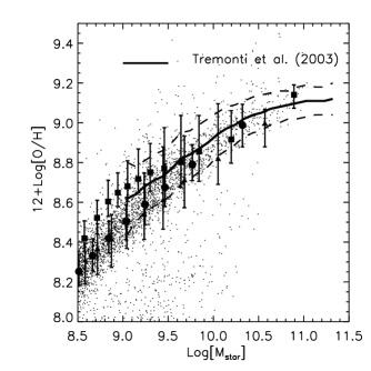
Figure 5: Metallicity–mass relation for our model galaxies (shown as points). The thick solid line represents the median relation between stellar mass and metallicity obtained for a sample of $50,000$ galaxies in the SDSS (Tremonti et al., in preparation). The dashed lines indicate the scatter in the observed relation. The solid symbols represent the median obtained from our models in bins containing $\sim 400$ galaxies each. Filled circles are for the retention model, filled triangles are for the ejection model and filled squares are for the wind model. The error bars mark the $20{\rm th}$ and $80{\rm th}$ percentiles of the distribution.

Figure 6: Relation between metallicity and rotational velocity for our model galaxies (shown as points). The filled squares represent the observational data from Garnett, (2002). The vertical dashed line in the panel corresponds to a velocity $120\,{\rm km}\,{\rm s}^{-1}$ (the turn–over velocity claimed by Garnett).

In Fig. 7 we show a comparison between the gas fraction of galaxies in our models and the gas fractions computed by Garnett, (2002). The same sample of objects as in Fig. 6 is plotted, both for the models and for the observations. Again our model agrees well with the observational data.

Figure 7: Gas fraction as function of the B–band luminosity for our model galaxies (shown as points). Filled squares are the gas fractions computed by Garnett, (2002) for the same sample of data shown in Fig. 6. Results are shown for the retention model, but are very similar for the other two schemes.

6 Chemical enrichment of the ICM

In our simulated cluster, the metallicity in the hot gas component is $\simeq 0.26$–$0.30~{}Z_{\odot}$ which is in good agreement with X–ray measurements (Renzini et al.,, 1993).

As pointed out by Renzini et al., simple metal abundances in the ICM depend not only on the total amount of metals produced in stars, but also on how much dilution there has been from pristine gas. A quantity that is not dependent on this effect or on the total mass in dark matter in the cluster is the so–called iron mass–to–light ratio (IMLR), defined as the ratio between the mass of iron in the ICM and the total B-band luminosity of cluster galaxies.

Our simulated cluster has a total mass of $1.14\cdot 10^{15}\,h^{-1}\,{\rm M}_{\odot}$ and a total luminosity in the B band of $\sim 10^{13}\,L_{\odot}$. Assuming a solar iron mass fraction from Grevesse, Noels & Sauval (1996), we find IMLR $=0.015-0.020\,{\rm M}_{\odot}\,L^{-1}_{\odot}$ for our three models, in agreement with the range given by Renzini et al., (1993).

Table 4 lists the total mass–to–light ratios of our cluster in the V and B–bands. The results are given for the three different feedback schemes. Note that the observational determination of a cluster mass–to–light ratio is not an easy task. Both the mass and the luminosity estimates are affected by uncertainties. Estimates based on the virial mass estimator give $\Upsilon_{\rm V}\sim 175$–$252$ (Carlberg et al.,, 1996; Girardi et al.,, 2000) while B–band mass–to–light ratios are in the range $200$–$400\,h^{-1}\,\Upsilon_{\odot}$ (Kent & Gunn,, 1982; Girardi et al.,, 2002). It has been argued that the virial mass estimator can give spurious results if substructure is present in the cluster or if the volume sampled does not extend out to the virial radius. In general, estimates based on masses derived from X–ray data tend to give lower values.

Table 4: Mass–to–light ratios in the V and in the B–band for our three models. The units are in $h\,\Upsilon_{\odot}$.

	$\Upsilon_{\rm B}$	$\Upsilon_{\rm V}$
retention	$290$	$230$
ejection	$250$	$200$
wind	$240$	$190$

The good agreement between the model predictions and the observational results indicates that our simulation may provide a reasonable description of the circulation of metals between the different baryonic components in the Universe. We now use our models to generate a set of predictions for when the metals in the ICM were ejected and for which galaxies were primarily responsible for the chemical pollution.

Recall that we assume that metals are recycled instantaneously and that the chemical pollution of the ICM happens through two routes:

• in the retention scheme the reheated mass (along with its metals) is ejected directly into the hot component. In this model, the enrichment of the ICM occurs at the same time as the star formation.

• In the ejection scheme the reheated material (along with its metals) stays for some time outside the halo and is later re–incorporated into the hot component. This means that there is a delay in the enrichment of the ICM in this scheme.

• The wind scheme sits somewhere in between the retention and ejection models. Metals are ejected out of the halo by galaxies that satisfy the outflow conditions. Otherwise, the metals are ejected directly into the hot gas.

The instantaneous recycling assumption means that the epoch of the production of the bulk of metals in the ICM coincides with the epoch of the production of the bulk of stars. In Fig. 8 we show the average star formation rate (SFR) of galaxies that end–up in the cluster region and the average star formation rate for galaxies that end–up in the field (the field is defined as consisting of all haloes outside the main cluster that are not contaminated by low resolution particles).

The SFRs in the two regions are normalised to the total amount of stars formed. The figure shows that star formation in the cluster is peaked at high redshift ($\sim 5$) and drops rapidly after redshift $3$. The peak of the SFR in the field occurs at lower redshift ($\sim 3$). The decline in star formation from the peak to the present day is also very much shallower in the field.

Integrating the SFR history of the cluster, we find that $\sim 85$ per cent of the stars in the cluster formed at redshift larger than $2$ and $\sim 70$ per cent at redshift larger than $3$. The corresponding values in the field are $60$ per cent and $40$ per cent. The results are similar in all the three models.

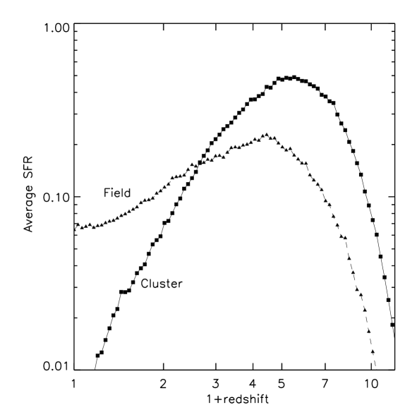
Figure 8: Average star formation rate as function of redshift in the cluster (solid line with filled squares) and in the field (dashed line with filled triangles).

As explained in Sec. 1, there is no general consensus on which galaxies were responsible for enriching the ICM. Several theoretical studies have proposed that mass loss from elliptical galaxies is an effective mechanism for explaining the observed amount of metals in the ICM. Some of these studies require an IMF that is skewed towards more massive stars at high redshift (Matteucci & Vettolani,, 1988; Gibson & Matteucci,, 1997; Moretti et al., 2003). Kauffmann & Charlot, (1998) used semi–analytic models to model the enrichment of the ICM and found that a significant fraction of metals come from galaxies with circular velocities less than $125\,{\rm km}\,{\rm s}^{-1}$. There have also been a number of more recent attempts to address this question in using hydrodynamic simulations (Aguirre et al.,, 2001; Springel & Hernquist,, 2003).

In a recent observational study, Garnett, (2002) has analysed the dependence of the so–called ‘effective yield’ on circular velocity for a sample of irregular and spiral galaxies (the data are compared to our model galaxies in Fig. 6), concluding, as Larson, (1974) had earlier, that galaxies with $V_{\rm rot}\leq 100-150\,{\rm km}\,{\rm s}^{-1}$ lose a large fraction of their SN ejecta, while galaxies above this limit retain most of their metals. As we have noted previously, this observational sample is limited both in number and in dynamic range.

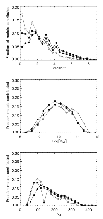
Figure 9: Fraction of metals, today present in the ICM, as a function of the redshift they were first incorporated into the intra–cluster gas (upper panel), as a function of the total mass of the ejecting galaxy (middle panel) and as a function of the virial velocity of the parent substructure (lower panel). Filled circles are used for retention model, empty circles are used for ejection model and filled squares are used for wind model.

Our model predictions are given in Fig. 9. The top panel shows the fraction of metals in the cluster at present day as a function of redshift they were first incorporated into the ICM. The other two panels show the fraction of metals as a function of the baryonic mass (middle) and the circular velocity (bottom) of the ejecting galaxies.

The expected delay in the chemical enrichment of the ICM is evident if one compares the ejection and wind models with the retention model in the top panel of the figure. Note that a similar delay is also seen in the metallicity of the hot component although it is very small because the reduction in total accreted ICM almost balances that in accreted metals. Over the redshift range $0$–$2$ the difference between the metallicity of the hot component in the retention and ejection schemes is only $1.5$ per cent solar. As expected, the behaviour of the wind model is intermediate between the ejection and retention schemes. We find that $60$–$80$ per cent of the metals are incorporated into the ICM at redshifts larger than $1$, $35$–$60$ per cent at redshifts larger than $2$ and $20$–$45$ per cent at redshifts larger than $3$ (we obtain lower values for the ejection scheme, higher values for the retention scheme and intermediate values for the wind model).

The middle panel shows that $43$–$52$ per cent of the metals are ejected by galaxies with total baryonic mass less than $1\times 10^{10}\,h^{-1}{\rm M}_{\odot}$. The distribution of the masses of the ejecting galaxies is approximatively independent of the feedback scheme. Although low mass galaxies dominate the luminosity function in terms of number, they do not dominate the contribution in mass. Approximately half of the contribution to the chemical pollution of the ICM is from galaxies with baryonic masses larger than $1\times 10^{10}\,h^{-1}{\rm M}_{\odot}$.

In our model, the star formation and feedback processes depend on the virial velocity of the parent substructure. In the bottom panel, we show the metal fraction as a function of the virial velocity of the ejecting galaxies. We find that $80$–$88$ per cent of the metals were ejected by galaxies with virial velocities less than $250\,{\rm km}\,{\rm s}^{-1}$. The ‘dip’ visible for the wind model in this panel corresponds to the sharp value of $V_{\rm crit}$ we adopt for this feedback scheme. Note that the results we find from this analysis are very similar to the results found by Kauffmann & Charlot, (1998), even though the modelling details are different.

7 Observational tests for different feedback schemes

Our analysis has shown that properties of galaxies at low redshifts are rather insensitive to the adopted feedback scheme after our free parameters have been adjusted to obtain a suitable overall normalisation.

The observational tests that would clearly distinguish between the different models are those that are sensitive to the amount of gas or metals that have been ejected outside dark matter haloes.

X–ray observations directly constrain the amount of hot gas in massive virialized haloes. The gas fraction tends to decrease as the X–ray temperature of the system goes down. David, Jones & Forman (1995) estimated that the gas–to–total mass fraction decreases by a factor $\sim 2$–$3$ from rich clusters to groups. In elliptical galaxies, the hot gas fraction is ten times lower than in rich clusters. These results were confirmed by Sanderson et al., (2003) in recent study of $66$ clusters and groups with X–ray data. One caveat is that the hot gas in groups is detected to a much smaller fraction of the virial radius than in rich clusters, so it is not clear whether current estimates accurately reflect global gas fractions (Loewenstein,, 2000). Another argument for why the gas fraction must decrease in galaxy groups comes from constraints from the soft X–ray background. If galaxy groups had the same gas fractions as clusters, the observed X–ray background at $0.25$ keV would exceed the observed upper limit by an order of magnitude (Pen,, 1999; Wu, Fabian & Nulsen, 2001).

Figure 10: Fraction of hot gas as a function of $M_{200}$. Solid circles represent the median and the error bars mark the $20{\rm th}$ and $80{\rm th}$ percentiles of the distributions.

In Fig. 10 we plot the gas fraction, i.e. $M_{\rm hot}/(M_{\rm hot}+M_{\rm vir})$, as a function of virial mass for all the haloes in our simulation. The mass of the hot gas is computed using Eq. 5. The results are shown for the case of a short re–incorporation timescale ($\gamma=0.3$) in the left column and for a long re–incorporation timescale ($\gamma=0.1$) in the right column. In this figure we plot results for the M2 simulation (see Table 1). Note that when we change $\gamma$, we also have to adjust the feedback efficiency $\epsilon$ so that the model has the same overall normalisation in terms of the total mass in stars formed (for $\gamma=0.3$, we assume $\epsilon=0.2$). We find that the gas fraction remains approximately constant for haloes with masses comparable to those of clusters, but drops sharply below masses of $10^{13}M_{\odot}$. As expected, the drop is more pronounced for the model with a long re-incorporation timescale.

The trends for the wind scheme are similar to those for the ejection scheme, but as can be seen, the ‘break’ towards lower gas fractions occurs at lower halo masses, because no material is ejected for haloes with circular velocities larger than $V_{\rm crit}$. In the ejection scheme, material is ejected for haloes up to a circular velocity of $350\,{\rm km}\,{\rm s}^{-1}$. Above this value, cooling flows shut down and no stars form in the central galaxies. Galaxies continue, however, to fall into the cluster. When a satellite galaxy is accreted, we have assumed that its ejected component is re–incorporated into the hot ICM. It is this infall of satellites that causes the gas fractions to saturate in all schemes at halo masses larger than a few times $10^{13}M_{\odot}$.

The ejection model with a long re–incorporation timescale is perhaps closest to satisfying current observational constraints. It reproduces the factor $2$–$3$ drop in gas fraction between rich clusters and groups. By the time one reaches haloes of $10^{12}M_{\odot}$, the gas fractions have decreased to a few percent. This may help explain why there has so far been a failure to detect any diffuse X-ray emission from haloes around late-type spiral galaxies (Benson et al.,, 2000; Kuntz et al.,, 2003). Note that in the retention model, we have assumed that the material reheated by supernovae explosions never leaves the halo. This translates into a hot gas fraction that is almost constant as a function of $M_{200}$. This model is therefore not consistent with the observed decrease in baryon fraction from rich clusters to galaxy groups.

Another possible way of constraining our different feedback schemes is to study what fraction of the metals reside in the diffuse intergalactic medium, well away from galaxies and their associated haloes. We now study how metals are partitioned among stars, cold gas, hot halo gas and the ‘ejected component’ and we show how this evolves as a function of redshift.

We plot the evolution of the metal content in the different components for our three different feedback schemes. For the ejection scheme we show results for two different re-incorporation timescales. The metal mass in each phase is normalised to the total mass of metals in the simulation at redshift zero. This is simply the yield Y multiplied by the total mass in stars formed by $z=0$. Note that in the retention scheme, all the reheated gas is put into the halo and there is no ejected component.

Fig. 11 shows the evolution of the metallicity for an average ‘field’ region of the Universe (our simulation M2). In contrast, Fig. 12 shows results for our cluster. In this plot we only consider the metals ejected from galaxies that reside within the virial radius of the cluster at the present day. We also normalise to the total mass of metals inside this radius, rather than the total mass of metals in the whole box. Because very little material is ejected from massive clusters in any of our feedback schemes, the ejected component always falls to zero by $z=0$ in Fig. 12.

Let us first consider the field simulation (Fig. 11). In the retention scheme, more than $70$ per cent of the metals are contained in the hot gas. About $20$–$30$ per cent of the metals are locked into stars and around $10$ per cent of the metals are in cold gas in galaxies. In the ejection scheme, a large fraction of the metals reside outside dark matter haloes. This is particularly true for the ‘slow’ re-incorporation scheme, where the amounts of metals in stars, in hot gas and in the ejected component are almost equal at $z=0$. For the ‘fast’ re-incorporation model, the metals in the hot gas still dominate the budget at low redshifts.

In the wind scheme, the amount of metals outside virialized haloes is considerably lower. There are a factor $2$ more metals in the hot gas than there are in stars at $z=0$.

Figure 11: Evolution of the metal content of different phases for the three different models used in this paper and for a typical ‘field’ region. In each panel the solid line represents the evolution of the metal content in the stars, the dashed line the cold gas, the dashed–dotted line the hot gas and the long–dashed line the ejected component (not present in the retention model). The metal content in each phase is normalised to the total mass of metals produced from all the galaxies considered.

At higher redshifts, the relative fraction of metals contained in cold galactic gas and in the ejected component increases. This is because galaxies are less massive and reside in dark matter haloes with lower circular velocities. As a result, they have higher gas fractions (see Sec. 4.2) and are able to eject metals more efficiently. In the ejection scheme, the material that is reheated by supernovae is always ejected from the halo, irrespective of the circular velocity of the system. In this scheme, metals in the ejected component (i.e. in diffuse intergalactic medium) dominate at redshifts greater than 2 in the case of fast re-incorporation and at all redshifts in the case of slow re-incorporation. In the wind scheme, material is only ejected if the circular velocity of the halo lies below some critical threshold. In this scheme, there are always more metals associated with dark matter haloes than there are in the ejected component.

Turning now to the cluster (Fig. 12), we see that the ejected component is negligible in all three schemes. The amount of metals outside dark matter haloes never exceeds the amount of metals locked up in stars up to redshift $\sim 3$. This is because dark matter haloes collapse earlier and merge together more rapidly in the overdense regions of the Universe that are destined to form a rich cluster. Although metals may be ejected, they are quickly re–incorporated as the next level of the hierarchy collapses. Note that the metals in the cold gas also fall sharply to zero at low redshifts. This is because galaxies that are accreted onto the cluster lose their supply of new gas. Stars continue to form and the cluster galaxies simply run out of cold gas.

Comparison of Fig. 11 with Fig. 12 suggests that cosmic variance effects will turn out to be important when trying to constrain different feedback schemes using estimates of the metallicity of the intergalactic medium deduced from, for example, CIV absorption systems in the spectra of quasars (e.g. Schaye et al.,, 2003). Nevertheless, the strong differences between our different feedback schemes suggest that these kinds of measurements will eventually tell us a great deal about how galaxies ejected their metals over the history of the Universe.

Figure 12: Same as in Fig. 11 but for the galaxies within the virial radius of our cluster simulation. Different lines have the same meaning as in Fig. 11.

Figure 13: Evolution of the different phases for the slow ejection scheme. The left panel shows the results for the galaxies within the virial radius of our cluster simulation, while the right panel shows the results for a typical ‘field’ region.

Finally, in Fig. 13 we show the evolution of the different phases for the slow ejection scheme, that can be considered as our ‘favourite’ model. In the left panel we plot the evolution in mass of the different phases for all the galaxies within the virial radius in our cluster simulation. In agreement with what is shown in Fig. 8, the stellar component grows very slowly after redshift $\sim 3$, when most of the stars in the cluster have already been formed. The cold gas and the ejected mass decrease as galaxies are accreted onto the cluster and stripped of their supply of new gas. The hot gas mass increases because of the accretion of ‘diffuse material’. In the right panel we plot the evolution of the mass density in each reservoir for our field simulation. Note that here the evolution in the stellar mass density is more rapid than in the field.

8 Discussion and Conclusions

We have presented a semi–analytic model that follows the formation, evolution and chemical enrichment of galaxies in a hierarchical merger model. Galaxies in our model are not closed boxes. They eject metals and we track the exchange of metals between the stars, the cold galactic gas, the hot halo gas and an ejected component, which we identify as the diffuse intergalactic medium (IGM).

We have explored three different schemes for implementing feedback processes in our models:

• in the retention model, we assume that material reheated by supernovae explosions is ejected into the hot halo gas.

• In the ejection model, we assume that this material is ejected outside the halo. It is later re–incorporated after a time that is of order the dynamical time of the halo.

• In the wind model, we assume that galaxies eject material until they reside in haloes with $V_{\rm vir}>V_{\rm crit}$. Ejected material is also re–incorporated on the dynamical time–scale of the halo. The amount of gas that is ejected is proportional to the mass of stars formed.

In all cases we can adjust the parameters to obtain reasonably good agreement between our model predictions and observational results at low redshift. The wind scheme is perhaps the most successful, allowing us to obtain remarkably good agreement with both the cluster luminosity function and the slope and zero–point of the Tully–Fisher relation. All our models reproduce a metallicity mass relation that is in striking agreement with the latest observational results from the SDSS. By construction, we also reproduce the observed trend of increasing gas fraction for smaller galaxies. The good agreement between models and the observational results suggests that we are doing a reasonable job of tracking the circulation of metals between the different baryonic components of the cluster.

We find that the chemical enrichment of the ICM occurs at high redshift: $60$–$80$ per cent of the metals are ejected into the ICM at redshifts larger than $1$, $35$–$60$ per cent at redshifts larger than $2$ and $20$–$45$ per cent at redshifts larger than $3$. About half of the metals are ejected by galaxies with baryonic masses less than $1\times 10^{10}\,h^{-1}{\rm M}_{\odot}$. The predicted distribution of the masses of the ejecting galaxies is very similar for all $3$ feedback schemes. Although small galaxies dominate the luminosity function in terms of number, they do not represent the dominant contribution to the total stellar mass in the cluster. Approximately the same contribution to the chemical pollution of the ICM is from galaxies with baryonic masses larger than $1\times 10^{10}\,h^{-1}{\rm M}_{\odot}$.

Finally, we show that although most observations at redshift zero do not strongly distinguish between our different feedback schemes, the observed dependence of the baryon fraction on halo virial mass does place strong constraints on exactly how galaxies ejected their metals. Our results suggest that gas and its associated metals must be ejected very efficiently from galaxies and their associated dark matter haloes. Once the material leaves the halo, it must remain in the diffuse intergalactic medium for a time that is comparable to the age of the Universe.

Future studies of the evolution of the metallicity of the intergalactic medium should also be able to clarify the mechanisms by which such wind material is mixed into the environment of galaxies.

References

- Aguirre et al., (2001) Aguirre A., Hernquist L., Schaye J., Weinberg D. H., Katz N., Gardner J., 2001, ApJ, 560, 599
- Baugh et al. (1996) Baugh C. M., Cole S., Frenk C. S., 1996, MNRAS, 283, 1361
- Benson et al., (2000) Benson A. J., Bower R. G., Frenk C. S., White S. D. M., 2000, MNRAS, 314, 557
- Binney & Tremaine, (1987) Binney J., Tremaine S., 1987, Galactic Dynamics, Princeton Univ. Press, Princeton
- Boissier et al., (2001) Boissier S., Boselli A., Prantzos N., Gavazzi G., 2001, MNRAS, 321, 733
- Bower et al. (1992) Bower R. G., Lucey J. R., Ellis R. S., 1992, MNRAS, 254, 589
- Bruzual & Charlot, (1993) Bruzual G., Charlot S., 1993, ApJ, 405, 538
- Cardelli et al. (1989) Cardelli J. A., Clayton G. C., Mathis J. S., 1989, 345, 245
- Carlberg et al., (1996) Carlberg R. G., Yee H. K. C., Ellingson E., Abraham R., Gravel P., Morris S., Pritchet C. J., 1996, ApJ, 462, 32
- Charlot et al. (1996) Charlot S., Worthey G., Bressan A., 1996, ApJ, 457, 625
- Chiosi et al., (1998) Chiosi C., Bressan A., Portinari L., Tantalo R., 1998, A&A, 339, 355
- Cole et al., (2000) Cole S., Lacey C. G., Baugh C. M., Frenk C. S., 2000, MNRAS, 319, 168
- Dahlem et al. (1998) Dahlem M., Weaver K., Heckman T. M., 1998, ApJS, 118, 401
- David et al. (1991) David L. P., Forman W., Jones C., 1991, ApJ, 380, 39
- David et al. (1995) David L. P., Jones C., Forman W., 1995, ApJ, 445, 578
- De Grandi & Molendi, (2001) De Grandi S., Molendi S., 2001, ApJ, 551, 153
- De Lucia et al., (2003) De Lucia G., Kauffmann G., Springel V., White S. D. M., Lanzoni B., Stoehr F., Tormen G., Yoshida N., 2003, MNRAS in press, preprint, astro-ph/0306205
- De Propris et al., (2003) De Propris R., Colless M., Driver S. P., Couch W., Peacock J. A., Baldry I. K., Baugh C. M., Bland-Hawthorn J., Bridges T., Cannon R., Cole S., Collins C., Cross N., Dalton G. B., Efstathiou G., Ellis R. S., Frenk C. S., Glazebrook K., Hawkins E., Jackson C., Lahav O., Lewis I., Lumsden S., Maddox S., Madgwick D. S., Norberg P., Percival W., Peterson B., Sutherland W., Taylor K., 2003, MNRAS, 342, 725
- Edge & Stewart, (1991) Edge A. C., Stewart G. C., 1991, MNRAS, 252, 414
- Efstathiou, (2000) Efstathiou G., 2000, MNRAS, 317, 697
- Ettori et al., (2002) Ettori S., Fabian A. C., Allen S. W., Johnstone M. N., 2002, MNRAS, 331, 635
- Fukumoto & Ikeuchi, (1996) Fukumoto J., Ikeuchi S., 1996, PASJ, 48, 1
- Garnett, (2002) Garnett D. R., 2002, ApJ, 581, 1019
- Gibson & Matteucci, (1997) Gibson B. K., Matteucci F., 1997, ApJ, 475, 47
- Gibson et al. (1997) Gibson B. K., Loewenstein M., Mushotzky R. F., 1997, MNRAS, 290, 623
- Giovanelli et al., (1997) Giovanelli R., Haynes M. P., Da Costa L. N., Freudling W., Salzer J. J., Wegner G., 1997, ApJ, 477, 1
- Girardi et al., (2000) Girardi M., Borgani S., Giuricin G., Mardirossian F., Mezzetti M., 2000, ApJ, 530, 62
- Girardi et al., (2002) Girardi M., Manzato P., Mezzetti M., Giuricin G., Limboz F., 2002, 569, 720
- Gnedin, (1998) Gnedin N. Y., 1998, MNRAS, 294, 407
- Grevesse et al. (1996) Grevesse N., Noels A., Sauval A. J., 1996, in ASP Conf. Series 99, ‘Standard Abundances’,117
- Gunn & Gott, (1972) Gunn J. E., Gott J. R., 1972, ApJ, 176, 1
- Heckman, (2002) Heckman T. M., 2002, in ASP Conf. Series 254, ‘Extragalactic Gas at Low Redshift’, 292
- Heckman et al., (1995) Heckman T. M., Dahlem M., Lehnert M. D., Fabbiano G., Gilmore D., Waller H., 1995, ApJ, 448, 98
- Heckman et al., (2000) Heckman T. M., Lehnert M., Strickland D., Armus L., 2000, ApJS, 129, 493
- Helly et al., (2003) Helly J. C., Cole S., Frenk C. S., Baugh C. M., Benson A., Lacey C., Pearce F. R., 2003, MNRAS, 338, 913
- Hernandez & Ferrara, (2001) Hernandez X., Ferrara A., 2001, MNRAS, 324, 484
- Jenkins et al., (2001) Jenkins A., Frenk C. S., White S. D. M., Colberg J. M., Cole S., Evrard A. E., Couchman H. M. P., Yoshida N., 2001, MNRAS, 321, 372
- see also Katz & White, (1993) Katz N., White S. D. M., 1993, ApJ, 412, 455
- Kauffmann & Charlot, (1998) Kauffmann G., Charlot S., 1998, MNRAS, 294, 705
- Kauffmann & Haehnelt, (2000) Kauffmann G., Haehnelt M., 2000, MNRAS, 311, 576
- Kauffmann et al. (1993) Kauffmann G., White S. D. M., Guiderdoni B., 1993, MNRAS, 264, 201
- Kauffmann et al., (1999) Kauffmann G., Colberg J. M., Diaferio A., White S. D. M., 1999, MNRAS, 303, 188
- Kauffmann et al., (2003) Kauffmann G., Heckman T. M., White S. D. M., Charlot S., Tremonti C., Peng E. W., Seibert M., Brinkmann J., Nichol R. C., SubbaRao M., York D., 2003, MNRAS, 341, 54
- Kennicutt et al. (2003) Kennicutt R. C., Jr., Bresolin F., Garnett D. R., 2003, ApJ, 591, 801
- Kent & Gunn, (1982) Kent S. M., Gunn J. E., 1982, AJ, 87, 945
- Kodama et al., (1998) Kodama T., Arimoto N., Barger A. J., Aragón-Salamanca A., A&A, 334, 99
- Kroupa & Boily, (2002) Kroupa P., Boily C. M., 2002, MNRAS, 336, 1188
- Kuntz et al., (2003) Kuntz K. D., Snowden S. L., Pence W. D., Mukai, K., 2003, ApJ, 588, 264
- Lacey & Cole, (1993) Lacey C., Cole S., 1993, MNRAS, 262, 627
- Lanzoni et al., (2003) Lanzoni B., Ciotti L., Cappi A., Tormen G., Zamorani G., 2003, ApJ in press, preprint astro-ph/0307141
- Larson, (1974) Larson R. B., 1974, MNRAS, 169, 229
- Larson, (1998) Larson R. B., 1998, MNRAS, 301, 569
- Larson & Dinerstein, (1975) Larson R. B., Dinerstein H. L., 1975, PASP, 87, 911
- Lehnert & Heckman, (1996) Lehnert M., Heckman T. M., 1996, ApJ, 462, 651
- Loewenstein, (2000) Loewenstein M, 2000, ApJ, 532, 17
- Macfarland et al., (1998) Macfarland T., Couchman H. M. P., Pearce F. R., Pichlmeier J., 1998, New Astronomy, 3, 687
- Mac Low & Ferrara, (1999) Mac Low M., Ferrara A., 1999, ApJ, 513, 142
- Marlowe et al., (1995) Marlowe A. T., Heckman T. M., Wyse R. F. G., Schommer R., 1995, ApJ, 438, 563
- Martin, (1996) Martin C. L., 1996, ApJ, 465, 680
- Martin, (1999) Martin C. L., 1999, ApJ, 513, 156
- Matteucci & Gibson, (1995) Matteucci F., Gibson B. K., 1995, A&A, 304, 11
- Matteucci & Vettolani, (1988) Matteucci F., Vettolani G., 1988, A&A, 202, 21
- Massey, (1998) Massey P., 1998, in Asp Conf. Series 142, ‘The Stellar Initial Mass Function’, 17
- McKee & Ostriker, (1977) McKee C. F., Ostriker J. P., 1977, ApJ, 218, 148
- Mo et al. (1998) Mo H. J., Mao S., White S. D. M., 1998, MNRAS, 295, 319
- Moretti et al. (2003) Moretti A., Portinari L., Chiosi C., 2003, A&A, 408, 431
- Mori & Burkert, (2000) Mori M., Burkert A., 2000, ApJ, 538, 559
- Mushotzky & Loewenstein, (1997) Mushotzky R. F., Loewenstein M., 1997, ApJ, 481, L63
- Mushotzky et al., (1996) Mushotzky R. F., Loewenstein M., Arnaud K., Tamura T., Fukazawa Y., Matsushita K., Kikuchi K., Hatsukade I., 1996, ApJ, 466, 686
- Navarro et al. (1995) Navarro J. F., Frenk C. S., White S. D. M., 1995, MNRAS, 275, 56
- Navarro et al. (1997) Navarro J. F., Frenk C. S., White S. D. M., 1997, ApJ, 490, 493
- Padmanabhan et al., (2003) Padmanabhan N., Seljak U., Strauss M. A., Blanton M. R., Kauffmann G., Schlegel D. J., Tremonti C., Bahcall N., Bernardi B., Brinkmann J., Fukugita M., Ivezić Z., preprint, astro-ph/0307082
- Pen, (1999) Pen U., 1999, ApJ, 510, 1
- Pettini et al., (2000) Pettini M., Steidel C. C., Adelberger K. L., Dickinson M., Giavalisco M., 2000, ApJ, 528, 96
- Pettini et al., (2001) Pettini M., Shapley A. E., Steidel C. C., Cuby J. G., Dickinson M., Moorwood A. F. M., Adelberger K. L., Giavalisco M., 2001, ApJ, 554, 981
- Renzini, (1997) Renzini A., 1997, ApJ, 488, 35
- Renzini et al., (1993) Renzini A., Ciotti L., Dercole A., Pellegrini S., 1993, ApJ, 419, 52
- Rocha-Pinto et al., (2000a) Rocha-Pinto H. J., Scalo J., Maciel W. J., Flynn C., 2000a, A&A, 358, 869
- Rocha-Pinto et al., (2000b) Rocha-Pinto H. J., Scalo J., Maciel W. J., Flynn C., 2000b, ApJ, 531, L115
- Salpeter, (1955) Salpeter E. E., 1955, ApJ, 121, 161
- Sanderson et al., (2003) Sanderson A. J. R., Ponman T. J., Finoguenov A., Lloyd–Davies E. J., Markevitch M., 2003, MNRAS, 340, 989
- e.g. Schaye et al., (2003) Schaye J., Aguirre A., Kim T., Theuns T., Rauch M., Sargent W. L. W., 2003, ApJ, 596, 768
- Schechter, (1976) Schechter P., 1976, ApJ, 203, 297
- Shapley et al., (2001) Shapley A. E., Steidel C. C., Adelberger K. L., Dickinson M., Giavalisco M., Pettini M., 2001, ApJ, 562, 95
- Simien & de Vaucouleurs, (1986) Simien F., de Vaucouleurs G., 1986, ApJ, 302, 564
- Somerville & Primack, (1999) Somerville R. S., Primack J. R., 1999, MNRAS, 310, 1087
- Somerville et al. (2001) Somerville R. S., Primack J. R., Faber S. M., 2001, MNRAS, 320, 504
- Spergel et al., (2003) Spergel D. N., Verde L., Peiris H. V., Komatsu E., Nolta M. R., Bennett C. L., Halpern M., Hinshaw G., Jarosik N., Kogut A., Limon M., Meyer S. S., Page L., Tucker G. S., Weiland J. L., Wollack E., Wright E. L., ApJS, 148, 175
- Springel & Hernquist, (2003) Springel V., Hernquist L., 2003, MNRAS, 339, 289
- Springel et al., (2001) Springel V., White S. D. M., Tormen G., Kauffmann G., 2001, MNRAS, 328, 726
- Sutherland & Dopita, (1993) Sutherland R. S., Dopita M. A., 1993, ApJS, 88, 253
- Tormen, (1997) Tormen G., 1997, MNRAS, 290, 411
- Tormen et al. (1997) Tormen G., Bouchet F. R., White S. D. M. 1997, MNRAS, 286, 865
- Wang & Heckman, (1996) Wang B., Heckman T. M., 1996, ApJ, 457, 645
- White & Frenk, (1991) White S. D. M., Frenk C. S., 1991, ApJ, 379, 52
- White et al., (1993) White S. D. M., Navarro J. F., Evrard A. E., Frenk C. S., 1993, Nature, 366, 429
- Wiebe et al. (1999) Wiebe D. S., Shustov B. M., Tutukov A. V., 1999, AA, 345, 93
- Wu et al. (2001) Wu K. K. S., Fabian A. C., Nulsen P. E. J., 2001, MNRAS, 324, 95
- Yoshida et al. (2001) Yoshida N., Sheth R. K., Diaferio A. 2001, MNRAS, 328, 669
- Yoshida et al., (2002) Yoshida N., Sthoehr F., Springel V., White S. D. M., 2002, MNRAS, 335, 762
- Zepf & Silk, (1996) Zepf S. E., Silk J., 1996, ApJ, 466, 114