Polarization & light curve variability: the “patchy-shell” model

Abstract

Recent advances in early detection and detailed monitoring of gamma-ray burst (GRB) afterglows have revealed variability in some afterglow light curves. One of the leading models for this behavior is the patchy shell model. This model attributes the variability to random angular fluctuations in the relativistic jet energy. These non axisymmetric fluctuations should also impose variations in the degree and angle of polarization that are correlated to the light curve variability. In this letter we present a solution of the light curve and polarization resulting from a given spectrum of energy fluctuations. We compare light curves produced using this solution with the variable light curve of GRB 021004, and we show that the main features in both the light curve and the polarization fluctuations are very well reproduced by this model. We use our results to draw constraints on the characteristics of the energy fluctuations that might have been present in GRB 021004.

1 Introduction

Within the Fireball model for gamma-ray bursts (GRB s) (Piran 2000, Mészáros 2002), the emission process in the optical and X-ray bands during the afterglow (AG) is most likely an optically thin, slow cooling synchrotron. Under the simplifying assumptions of spherical or scale free axial symmetry, this model predicts a smooth, broken power-law light curve. Until recently most all of the observed AGs exhibited a light curve conforming to the above predictions of the model. However, recently several observed AGs (mainly GRB 021004 and GRB 030329) showed variable light curves that can be interpreted as fluctuations superimposed on a power law decay. These two AGs were recorded with especially good resolution and accuracy, and they were detected very shortly after the GRB. Thus it is not clear to what extent the compatibility of earlier AG observations with a broken power-law indicates an intrinsic agreement (as opposed to sparse sampling).

Fluctuating light curves were predicted by various models. The most plausible models suggest variations in the blast wave’s energy or in the external density. These variations can be (locally) spherically symmetric as in the energy fluctuated refreshed shocks model (Rees & Mészáros 1998, Kumar & Piran 2000a, Sari & Mészáros 2000), or they can be aspherical variations of the energy (as in the patchy-shell model; Kumar & Piran 2000b) or the external density (Wang & Loeb 2000, Lazzati et al. 2002, Nakar et al. 2003). Motivated by the clear evidence for deviations from axisymmetry in at least one burst (GRB 021004) we focus our attention on the aspherical models. In this letter, we investigate the patchy-shell model.

In the patchy-shell model the energy per solid angle of the blast wave displays angular variations. These energy variations induce fluctuations in the AG light curve. Because of the non axisymmetric nature of the energy variations they also impose variations in the degree and angle of polarization that are correlated to the light curve variability (Granot & Königel 2003). We calculate the light curve and the polarization resulting from a given spectrum of energy fluctuations. We show that generally the variability time scale $\Delta T$ behaves as $\Delta T\sim T$, and the amplitude envelope decays as $T^{-3/8}$, where $T$ is the time in the observer frame. We also find a correlation and time delay between light-curve variations in different spectral bands. Current observations restrict the amplitude of energy fluctuations to be less than a factor of $10$ (otherwise we would not expect the observed narrow distribution of $\gamma$-ray emission energy; Frail et al. 2001). We show here that such energy variations are consistent with the observations, namely that they can produce both variable and smooth light curves, depending on the observer location. Piran (2001) even argues that such fluctuations may solve the puzzle of why the energy emitted in $\gamma$-rays seems larger than the kinetic energy that remains in the blast-wave, whereas the opposite is expected.

GRB 021004 has all the properties expected from a non spherically symmetric burst: Its AG displays steep decays on time scales that cannot be obtained in a spherically symmetric model (Nakar & Piran 2003) and its polarization shows rapid fluctuations in the polarization angle and degree (Rol et al. 2003). These fluctuations cannot be explained by any of the current models, providing further indication that the radiation source is non axisymmetric (Lazzati et al. 2003). These fluctuations in the polarization were even predicted by Granot & Königel (2003) (based on the variable light curve and the expected axisymmetry break) prior to the observational report. We demonstrate that the patchy-shell model is capable of explaining the light-curve and polarization (amplitude and angle) of GRB 021004 and we determine the properties of the angular energy distribution that can account for the observed behavior.

In §2 we calculate the light curve and polarization from a patchy shell. In §3 we find an energy profile that reproduces the observed light curve and polarization of GRB 021004. We draw our conclusions in §4.

2 The light curve and polarization calculation

We calculate the observed light curve, degree of polarization and polarization angle, resulting from a synchrotron emission of an adiabatic blast wave with angular fluctuations in the energy, $E=E(R,\theta,\phi)$, where $E$ is the energy per solid angle . We assume that the energy of both the electrons and the magnetic field are in constant equipartition with the total internal energy of the shocked fluid and we take the circum-burst medium density as a constant (interstellar medium). Based on the thin shell nature of the Blandford & Mckee (1976) solution ($R/\Delta R\approx 16{\gamma}^{2}$, where $\gamma$ is the Lorentz factor of the freshly shocked fluid), we approximate the radiating region to be only the instantaneous shock front.

In interstellar medium (ISM), an adiabatic blast wave propagates at a Lorentz factor $\Gamma\propto R^{-3/2}$ ($\Gamma=\sqrt{2}\gamma$). Since $\theta_{s}$, the angular size of regions at radius $R$ causally connected by sound waves that propagate at $\beta_{s}=1/\sqrt{3}$ (in the fluid rest frame) grows as $d\theta_{s}=\beta_{s}dR/(\Gamma R)$, we obtain:

$$\theta_{s}(R)=\frac{2\beta_{s}}{3}\frac{1}{\Gamma}\approx\frac{1}{4\gamma}.$$ (1)

As long as the typical angular size of the energy fluctuations, $\theta_{fl}$, is larger than $\theta_{s}$, the energy profile is “frozen” in time ($E=E(\theta,\phi)$). Moreover, Kumar and Granot (2003) have shown that the actual transversal velocities of the fluid may be much smaller than the speed of sound. Consequently, the “frozen shell” approximation may remain valid even when $\theta_{s}\gtrsim\theta_{fl}$. Following these arguments, we carry out our calculation using the “frozen shell” approximation, which facilitates our calculation considerably, as we can treat each element of solid angle as part of a homogeneous sphere.

Under the above approximations, the contribution to the flux per unit of observer frequency $\nu$ from an element of solid angle $d\Omega$ at radius $R$ is given by (Sari 1998):

$$dF_{\nu}(R,\theta,\phi)\propto L^{\prime}_{\nu\gamma(1-\beta\cos\theta)}[\gamma(1-\beta Cos\theta)]^{-3}d\Omega,$$ (2)

where $L^{\prime}_{\nu^{\prime}}(R)$ is the luminosity of the solid angle element in the fluid rest frame. Calculating $L^{\prime}_{\nu^{\prime}}$ following the procedure of Sari, Piran and Narayan (1998) for the slow cooling regime we obtain:

$$dF_{\nu}(T,\theta,\phi)\propto\left(\frac{1+y}{\gamma}\right)^{-(3+\alpha)}d\Omega\left\{\begin{array}[]{c}E^{\frac{3}{4}}T^{\frac{3}{4}}(y+1/8)^{-\frac{3}{4}}\;\ \ \ \ \ \ \ \ \ \ \ \ \nu<\nu_{m}\\ E^{\frac{11+3p}{16}}T^{\frac{15-9p}{16}}(y+1/8)^{\frac{9p-15}{16}}\;\ \ \ \ \ \ \ \nu_{m}<\nu<\nu_{c}\\ E^{\frac{6+3p}{16}}T^{\frac{14-9p}{16}}(y+1/8)^{\frac{9p-14}{16}}\;\ \ \nu_{c}<\nu\end{array}\right.,$$ (3)

where $\alpha$, the spectral power law index, is equal to $-1/3,(p-1)/2$ and $p/2$ in each segment respectively. We have used here the definition $y\equiv(\gamma\theta)^{2}$ and $\theta\ll 1$. We also use the adibacity of the blast wave ($E\propto R^{3}\gamma^{2}$) that yields (Sari 1998) $R\propto(ET/(y+1/8))^{1/4}$ for any solid angle element. The angular dependence is implicit in $E$ and $y$ through the expression:

$$\gamma=3.6(1+8y)^{3/8}(E/10^{52})^{1/8}n^{-1/8}T_{d}^{-3/8}.$$ (4)

Now, the total observed flux, $F(T)$, is easily calculated by integration over the solid angle.

Having obtained the flux contribution per solid angle element we are able to calculate the linear polarization ($V=0$) as well. The total stokes parameters are simply the average of the local stokes parameters weighted by the flux :

$$\frac{\left\{\begin{array}[]{c}Q\\ U\\ \end{array}\right\}}{I\Pi_{synch}}=\frac{\int dF_{\nu}\Pi(y)\left\{\begin{array}[]{c}\cos(2\theta_{p})\\ \sin(2\theta_{p})\\ \end{array}\right\}}{\int dF_{\nu}},$$ (5)

where $\Pi_{synch}$ is the polarization of synchrotron emission in the fluid frame at the relevant power-law segment (Granot 2003, for $\nu_{m}<\nu<\nu_{c}$ it is $(p+1)/(p+7/3)$), $\theta_{p}$ is the polarization angle and $\Pi$ is the observed local polarization relative to $\Pi_{synch}$. Note that the integration over $dF$ is actually an integration over $d\Omega$. $\Pi$ and $\theta_{p}$ at each element depend on two factors: (i) The Lorentz boost of a photon emitted from that element and reaching the observer, which depends on $y$ (note that $y$ depends on $T$ and $E$, and thus on $\theta$ & $\phi$ (Eq.(4)), and (ii) the magnetic field configuration - random or uniform. A Random $B$ is described by the level of anisotropy, $b\equiv 2\langle B_{\parallel}^{2}\rangle/\langle B_{\perp}^{2}\rangle$ (Granot & Königel 2003), where $B_{\parallel}$ is a random component in the plane of the shock and $B_{\perp}$ is the component parallel to the propagation of the fluid. In this case $\Pi(y)/\Pi_{synch}\approx 2y(b-1)/((1+y)^{2}+2y(b-1))$ (Gruzinov 1999, Sari 1999, Granot 2003) and $\theta_{p}$ is radial [tangential] for $b<1$ [$b>1$]. In Uniform $B$, $\Pi=1$ is constant and $\theta_{p}$ is given in Granot & Königel (2003).

Although we are concerned with angular fluctuations, it is illuminating to consider first the spherically symmetric case. In this case the contribution to the observed flux at a given observer time is concentrated within a ring centered on the line of sight (Naturally all observed quantities here are independent of $\phi$). The flux under these conditions is given by a self similar function of $\theta$, $\xi(\theta)\equiv dF_{\nu}/d\theta$, when $\theta$ is measured in units of $(T^{3}nm_{p}c^{5}/E)^{1/8}$ and its height is normalized. Fig. (1) depicts $\xi$ for the three different spectral power law segments. $\xi$ is localized with FWHM of 0.5[1]$\theta_{max}$ for $\nu>\nu_{m}[\nu<\nu_{m}]$, where $\theta_{max}$ is the angle of maximum $\xi$. $\xi$ depends weakly (as $E^{1/8}$) on the energy, so in the case of a non-spherical energy distribution, as long as the energy variations are not large the shape of the observed ring is only mildly distorted. This analysis enables us to derive a constraint on the time scale of fluctuations in the light curve. A significant fluctuation can occur only after the ring is displaced such that it covers an essentially new region. As the FWHM is of the order of $\theta_{max}$, and with the power law dependence of $\theta_{max}$ on $T$, this takes place on time scales of the order of $T$. Thus, the time scale $\Delta T$ for fluctuations in a light curve produced by a patchy shell obeys the simple rule $\Delta T\gtrsim T$. One can understand this result in terms of angular and radial times. Although the angular time of a spot may be $<T$, its radial time, which is determined by the time over which the ring crosses a spot, is of the order of $T$. Naturally, no fluctuations are expected as long as $\theta_{fl}>\theta_{max}$. Hence, $\Delta T\sim max\{T,0.025[0.05](E/10^{52})^{1/3}n^{-1/3}(\theta_{fl}/0.03)^{8/3}\rm days\}$ for $\nu>\nu_{m}[\nu<\nu_{m}]$. Also, in case $\theta_{fl}$ is much smaller than $\theta_{max}$ (at late times, in case the frozen shell approximation still holds) we would expect to see small time scale fluctuations, which “survive” the smoothing effect, superimposed on the main features. However these fluctuations turn out to be so weak as to be completely hidden under the larger scale structures.

A few other properties that can be drawn from the behavior of $\xi$ (see Fig. 1) are: (i) The value of the Lorentz factor at $\theta_{max}$, $\gamma_{max}\equiv\gamma(\theta_{max})$, which can be regarded as the characteristic Lorentz factor at time $T$ for $\nu>\nu_{m}[\nu<\nu_{m}]$ is:

$$\gamma_{max}=7.7[5](E/10^{52})^{1/8}n^{-1/8}T_{d}^{-3/8}.$$ (6)

(ii) The relation $\gamma_{max}\theta_{max}=0.9[0.45]$ for $\nu>\nu_{m}[\nu<\nu_{m}]$ is constant, owing to the self-similarity of $\xi$. (iii) The overall amplitude of the fluctuations decreases as the square root of the number of observed spots and is $\propto\theta_{fl}/\theta_{max}\propto T^{-3/8}$ (Nakar et al. 2003). (iv) The fluctuations at the three power law segments $\nu_{m}<\nu<\nu_{c}$, $\nu_{c}<\nu$ and $\nu<\nu_{m}$ are correlated, but the first two are simultaneous while the fluctuations in the third segment are delayed relative to them by approximately $\Delta T$.

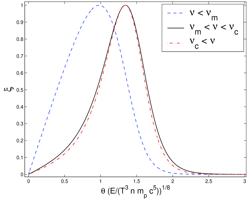
Figure 1: The function $\xi(\theta)$ for the three spectral power law segments. In this figure $p=2.2$, but $\xi$ is almost insensitive to $p$ in the range $2<p<3$.

3 GRB 021004

The AG of GRB 021004 was observed on October 4’th 2002 at a redshift of 2.32. The early optical detection (Fox et al. 2002), $T\sim 0.005\rm days$, enabled a detailed observation of this afterglow from a very early stage. This unusual afterglow shows clear deviations from a smooth temporal power law decay. A first bump is observed at $T\sim 0.05\rm days$, this bump is followed by a very steep decay. Another smaller bump is observed at $T\sim 0.8\rm days$ and a possible third one at $T\sim 3\rm days$. A steepening that may be a jet break is observed at $T\sim 4-7\rm days$. During the first two days the optical spectrum is rather constant (Pandey et al. 2003). Later, during the third bump and the start of the break, the AG shows color variations (Matheson et al 2003, Bersier et al 2003). This peculiar AG shows rapid polarization fluctuations as well (both in degree and angle). Between 0.3-0.8 days the polarization shows a fast drop and rise combined with a rotation of $60^{o}$ (Rol et al 2003, Covino et al. 2002a; Wang et al. 2003). These fluctuations are correlated to the light curve’s fluctuations: at 0.3 days the light curve is at the steep decay after the first bump while after 0.6 days it is at the rise of the second bump. Another measurement after $\sim 4\rm days$ shows another drop in the polarization level and a rotation of $30^{o}$ (Covino et al. 2002b). While the last measurement is taken at the beginning of the jet break and might be the result of a jet seen off axis (Gruzinov 1999; Ghisellini & Lazzati 1999; Sari 1999; Rossi et al. 2002), the earlier measurements are taken long before the jet break time and cannot be attributed to any of these models. These models are unable to explain the observed rotation (Lazzati et al 2003). The existence of rapidly varying polarization at such early stages indicates that the axisymmetry of the flow is broken in a non-regular manner on small angular scales. Here (fig 2) we show that the patchy shell model can produce a variable light curve and polarization and especially the angle rotation.

Several different mechanisms were suggested to explain this light curve (Lazzati et al. 2002; Nakar et al. 2003; Holland et al. 2003; Pandey et al. 2002, Bersier et al. 2003; Schaefer et al. 2003; Heyl & Perna 2003; Li & Chevalier 2003,Kobayashi, S. & Zhang 2002). Nakar & Piran (2003) have shown that as a result of angular effects none of the suggested spherical symmetric mechanisms can produce the steep decay ($\sim t^{-1.5}$) observed after the first bump. This implied lack of spherical symmetry is strongly supported by the polarization observations. Here we consider a symmetry break by a patchy shell. Within this model the most natural magnetic field configuration that produces correlated fluctuations in the light curve and the polarization is the random field (see §2).

We have applied the solution presented in Eqs. 3 & 4 in a search for a reasonable angular energy distribution that simultaneously produces the observed optical (R-band) light curve and polarization. We expect such a distribution to have a single characteristic angular scale $\theta_{fl}=\pi/k_{max}$ and a contrast on the order of a few, as was argued above. A random set of components was selected in two dimensional Fourier space, with a cutoff at $k_{max}$ and a power law spectral envelope $k^{s}$. The logarithmic contrast $c$ was defined such that $r.m.s.(log_{c}(E/E_{0}))=1$, where $E_{0}$ is the typical energy. We compare our results to the observed light curve during the first two days. We assume that during this time the optical band is between $\nu_{m}$ and $\nu_{c}$. The color changes during the third bump and the following jet break prevent us from applying our solution to later times.

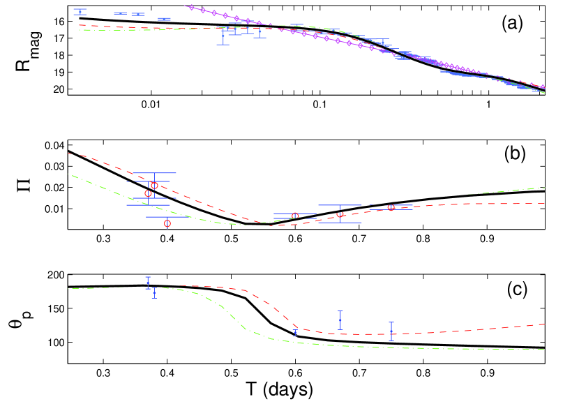
Figure 2: The light curve (upper panel), polarization level (middle panel) and angle (lower panel) obtained from three different random energy distributions vs. the observations of GRB 021004 ( light curve: Fox et al. 2003, Uemura et al. 2003, Pandey et al. 2003, Holland et al. 2003, Bersier et al. 2003; polarization (after ISM correction: Rol et al 2003, Covino et al. 2002a; Wang et al. 2003). The straight line (marked with diamonds) in the upper panel is a light curve obtained from an energy distribution randomly generated using the same parameters. The same AG may appear either as a smooth or fluctuating power-law to different observers.

Our strategy in trying to find a match between the model and the observed light curve was to scan the $\{k_{max},c,s\}$ parameter space and try to find the most suitable set of parameters. According to $X$ and $\gamma$ ray observations we have used throughout $p=2.2$ and $E_{0}=6\cdot 10^{52}$ergs. For each such set we produced $\sim 100$ synthetic light curves. Each point in this parameter space produces light curves with characteristic time and amplitude scales. An agreement to the scales observed in GRB 021004 was apparent in a relatively small neighborhood of parameters, namely $\theta_{fl}\approx 0.017\rm rad$ (the wave length of the fluctuations is $\approx 0.035\rm rad$ and $k_{max}\approx 185\rm rad^{-1}$), sharp spectrum, $s>2$, and a contrast of $2.5<c<5$. These results are similar to the one obtained by Nakar et al. 2003 with a much simpler model. We then visually selected from the light curves in this neighborhood (covering $\sim$ 1000 simulated lightcurves) three of those best fitting the observed light curve, which are displayed in fig. 2. Very reassuringly, those three energy profiles produce also a good fit to the observed polarization (see fig. 2b). In agreement with the observations, the polarization angle rotates by $45^{o}-80^{o}$ between 0.3-0.7 days (fig 2c). When fitting the polarization $b$, the anisotropy parameter, is a free parameter. We find that in order obtain the observed level of polarization $b\approx 0.5-0.8[1.25-2]$ if the magnetic field is mainly planar [parallel]. This $b$ decreases the level of polarization by a factor of $3-7$ compared to the maximal polarization obtained with $b=\infty$, and this result is consistent with the low observed value of polarization usually seen near the time of the jet break ($<3\%$) compared to the expected value of $10-20\%$ (Sari 1999, Ghisellini & Lazzati 1999). The obtained value of $k_{max}$ justifies our “frozen shell” approximation. After two observer days $\Gamma\approx 10$, hence $\theta_{fl}\gtrsim\theta_{s}\approx 1/40$ at all time ($T<2\rm days)$.

4 Conclusion

Of the various models suggested to deal with fluctuations in GRB AGs, we have dealt here with the ”patchy shell” model. The variability in this model results from the angular inhomogeneity of energy in a shock-wave expanding into the circum-burst medium. The time scale of these fluctuations is constrained to grow linearly with time, namely $\Delta T\sim T$, regardless of the angular scale of energy fluctuations in the shell. There is also an amplitude decay, inherent in the smoothing effect, which $\propto T^{-3/8}$. Another feature of this model is a variable degree and direction of polarization resulting from the azimuthal variation of the energy. The degree of polarization can reach an order of tens of percents in the case of very anisotropic magnetic fields.

As time progresses in the observer frame, radiation arrives from larger $\theta$’s. Changes in the flux and polarization occur when a group of fluctuations with a certain averaged orientation is replaced by a new group with a different averaged orientation because of this change in the observed region. Therefore the transition from one peak to the next in the light curve will characteristically be accompanied by a rotation of polarization, with a drop in polarization degree when the two groups contribute equally to the flux. This drop will be less pronounced the closer the polarization angle before and after the transition is. Thus, the polarization variations are correlated to the flux variations and occur on similar time scales. Note, however, that a large rotation can take place on much shorter time scales.

The light curve and polarization of GRB 021004 are in agreement with these general properties. Furthermore, we calculated a number of light and polarization curves from a set of randomly generated energy profiles and found recurring agreement between some of them and the observed data. This model, however, fails to explain the very short ($\sim 1h$) time scale variations that might have been observed at $T\sim 1\rm day$ (Bersier et al. 2003), at least as long as the frozen shell approximation holds, and there are no radial variations in the energy.

An important prediction arising from the self similar flux profile is a logarithmic time lag between light curve and polarization variations below and above $\nu_{m}$. A more accurate analysis of this problem, which we are currently carrying out, can be made by taking into account the finite thickness and the hydrodynamic profile of the radiating area and performing a three dimensional integration of the flux originating from different radii.

We would like to thank Re’em Sari and Davide Lazzati for helpful discussions. We especially thank Tsvi Piran for insightful remarks. The research of EN was partially supported by the Horowitz foundation and by the generosity of the Dan David prize by the Dan David scholarship 2003.

References

- (1) Bersier, D. et al., 2003, ApJL, 584, L43
- (2) Blandford, R. D., & Mckee, C. F., 1976, The physics of Fluids 19, 1130
- (3) Covino, S. et al., 2003a, GCN circ. 1595
- (4) Covino, S. et al., 2003b, GCN circ. 1622
- (5) Fox et al., 2003 Nature, 422, 284
- (6) Frail, D. A., et al., 2001, ApJL, 562 L55
- (7) Ghisellini, G. & Lazzati, D., 1999, MNRAS., 309 L7
- (8) Granot & Königel, 2003, ApJL 594, L83
- (9) Granot, J., 2003, 2003, ApJ, 596, L17
- (10) Gruzinov, A., 1999, ApJL, 525 L29
- (11) Heyl, J. & Perna, R., 2003, ApJL, 586, L13
- (12) Holland, S. et al., 2003, AJ, 125, 2291
- (13) Kobayashi, S. & Zhang, B., 2002, ApJL, 582, L7
- (14) Kumar, P., & Piran, T., 2000a ApJ, 532, 286
- (15) Kumar, P.,& Piran, T., 2000b, ApJ, 535, 152
- (16) Kumar, P. & Granot, ., 2003, ApJ, 591, 1075
- (17) Li, Z. & Chevalier, R. A., 2003, ApJL, 589, L69
- (18) Lazzati, D., Rossi, E., Covino, S., Ghisellini, G., & Malesani D., 2002, AA, 396, L5
- (19) Lazzati, D. et al., 2003, A&A, 410, 823
- (20) Matheson, T. et al., ApJL, 2003, 582, L5
- (21) Mészáros, P. 2002, ARA&A, 40, 137
- (22) Nakar, E. , Piran, T, & Granot, J., 2003, New Astronomy, 8, 495
- (23) Nakar E., & Piran T., 2003, ApJ, 598, 400
- (24) Nakar, E., Piran, T. & Waxman, E. 2003, JCAP, 10, 05
- (25) Pandey, S. B. et al. 2002, BASI, 31, 19
- (26) Piran, T. 2000, Phys. Rep. 333, 529.
- (27) Piran, T. 2001, astro-ph/0111314
- (28) Rees, M. J.& Mészáros, P., 1998, ApJL, 496, L1
- (29) Rol, E. et al. 2003, A&A, 405, L23
- (30) Rossi, E., Lazzati, D., Salmonson, J. D. & Ghisellini G., 2002, astro-ph/0211020
- (31) Sari, R., 1998, ApJL, 494L, 49
- (32) Sari, R., Piran, T., & Narayan, R., 1998, ApJL, 497, L17
- (33) Sari, R., 1999, ApJ 542 L43
- (34) Sari, R. & Mészáros, P., 2000, ApJL, 535, L33
- (35) Schaefer, B. et al., 2003, ApJ, 588, 387
- (36) Uemura, M., Kato, T., Ishioka, R. & Yamaoka, H., PASJ, 55, L31
- (37) Wang, X. & Loeb, A., 2000, ApJ, 535, 788
- (38) Wang, L., Baade, D., Hoeflich, P. & Wheeler, J. C., 2003, Submitted to ApJ, (astro-ph/0301266)