Phase analysis of the 1-year WMAP data and its application for the CMB foreground separation

Abstract

We present a new method based on phase analysis for the Galaxy and foreground component separation from the cosmic microwave background (CMB) signal. This method is based on a prevailing assumption that the phases of the underlying CMB signal should have no or little correlation with those of the foregrounds. This method takes into consideration all the phases of each multipole mode ($\ell\leq 50$, $-\ell\leq m\leq\ell$) from the whole sky without galactic cut, masks or any dissection of the whole sky into disjoint regions. We use cross correlation of the phases to illustrate that significant correlations of the foregrounds manifest themselves in the phases of the WMAP 5 frequency bands, which are used for separation of the CMB from the signals. Our final phase-cleaned CMB map has the angular power spectrum in agreement with both the WMAP result and that from Tegmark, de Oliveira-Costa and Hamilton (TOH), the phases of our derived CMB signal, however, are slightly different from those of the WMAP Internal Linear Combination map and the TOH map.

1 Introduction

The release of the first year results from the Wilkinson Microwave Anisotropy Probe (WMAP ) opens a new epoch of the full-sky CMB investigation, particularly for the analysis of different foreground components (Bennett et al., 2003a, b, c; Hinshaw et al., 2003a, b). The analyses from different groups, apart from the WMAP results, have raised two main issues: firstly, why is the power of the quadrupole component of the CMB signal considerably suppressed? (Tegmark, de Oliveira-Costa & Hamilton, 2003; de Oliveira-Costa, Tegmark, Zaldarriaga & Hamilton, 2003; Efstathiou, 2003) Secondly, is the CMB signal Gaussian? (Komatsu et al., 2003; Chiang, Naselsky, Verkhodanov & Way, 2003; Park, 2003; Eriksen et al., 2003) The key point to these questions may lie in the area of component separation, related with the removal of the foregrounds from the all frequency maps.

The WMAP group produced an Internal Linear Combination (ILC) map (Bennett et al., 2003c) using a weighted combination of the 5 bands outside the Galactic plane. Tegmark, de Oliveira-Costa & Hamilton (2003) (hereafter TOH) perform an independent foreground analysis from the WMAP data using weighting coefficients dependent not only on the angular scales ($\ell$) but also on the Galactic latitudes.

In this paper we propose an alternative method with the assumption that the phases of the CMB signal derived from foreground cleaning should correlate as little as possible with those of the foregrounds. According to the simplest inflation theory (see for review Komatsu et al. 2003), pure CMB signals constitute a Gaussian random field, which have random and uniformly distributed phases. Because of the pronounced non-Gaussianity of the foregrounds, it therefore becomes straightforward to regard the non-Gaussianity, if detected, from the WMAP Internal Linear Combination (ILC) map, the TOH maps or any other derived maps from the WMAP data as contaminations of the foregrounds at various levels. As such, we should have significant cross-correlations between the phases of the foregrounds and the CMB signal.

We perform the phase analysis of the signals for all the K–W bands of the WMAP in order to remove the Galaxy and extragalactic foregrounds. Below we will call our derived map the Phase–Cleaned Map (PCM), and our method the PCM method. Different from other methods for component separation, our method is based significantly on the properties of phases, using each map from the WMAP K–W bands as an image without any assumptions about the statistical nature of the CMB signal. Moreover, we use the whole sky for analyses and do not apply any Galaxy plane cut-off and masks, nor do we dissect the whole sky into disjoint regions. Our work is closely related with Chiang & Coles (2000); Chiang (2001); Naselsky, Novikov & Silk (2002); Chiang, Coles & Naselsky (2002) and Chiang, Naselsky, Verkhodanov & Way (2003), from which some of the aspects of the CMB phase analysis were developed. A new element is to implement the phases of the maps from multifrequency K–W bands for reconstruction of the PCM.

The layout of this paper is as follows. In Section 2 we describe the phases of the WMAP and illustrate the cross correlations between the foreground maps provided in the WMAP website and between the 5 frequency maps. We introduce the “non-blind” PCM method in Section 3 and in Section 4 we introduce the “blind” PCM method and elaborate the 4 steps for foreground cleaning. We use a set of simulated maps, which we call the wmap simulator as the numerical test on the “blind” PCM method. We produce the PCM using the “blind” method in Section 7 and compare the PCM map and the power spectrum with those of the WMAP ILC map and the TOH foreground-cleaned map and Wiener-filtered map. We perform the Gaussianity test on these maps in Section 8 and the Conclusion and Discussions are in Section 9.

2 The phases of the CMB and foregrounds

The statistical characterization of the temperature fluctuations of CMB plus foregrounds radiation and the instrumental noise on a sphere can be expressed as a sum over spherical harmonics:

$$\Delta T(\theta,\varphi)=\sum_{\ell=0}^{\infty}\sum_{m=-\ell}^{\ell}a_{\ell m}Y_{\ell m}(\theta,\varphi),$$ (1)

where $a_{\ell m}$ are the coefficients of the expansion. Homogeneous and isotropic CMB Gaussian random fields (GRFs), as a result of the simplest inflation paradigm, possess Fourier modes whose real and imaginary parts are Gaussian and mutually independent. The statistical properties are then completely specified by its angular power spectrum $C_{\ell}^{cmb}$,

$$\langle a^{cmb}_{\ell m}(a^{cmb})^{*}_{\ell^{{}^{\prime}}m^{{}^{\prime}}}\rangle=C_{\ell}^{cmb}\;\delta_{\ell\ell^{{}^{\prime}}}\delta_{mm^{{}^{\prime}}}.$$ (2)

In other words, from the Central Limit Theorem their phases

$$\Psi^{cmb}_{\ell m}=\tan^{-1}\frac{\Im(a_{\ell m}^{cmb})}{\Re(a_{\ell m}^{cmb})}$$ (3)

are randomly and uniformly distributed at the range $[0,2\pi]$. We hereafter denote at superscript “cmb” as the pure CMB signal. For the combined signal from the CMB and foregrounds we can write down

$$a_{\ell m}=|a_{\ell m}|\exp(i\Psi_{\ell m}),$$ (4)

where $|a_{\ell m}|$ is the modulus and $\Psi_{\ell m}$ is the phase of each $a_{\ell m}$ harmonic.

The statistical properties of the foreground signals are different from those of GRFs. In the contemporary CMB experiments the measured signals have contaminations from our Galaxy as well as from other extragalactic sources at all frequency bands. For example, for the K–Ka bands of the WMAP the foreground emissivity is mainly determined by the combination of the synchrotron and free-free emissions. For higher frequency bands (Q, V and W bands) the contaminations include the free-free and dust components and some of the residues from the synchrotron radiation. Using different assumption on the properties of the foregrounds such as the frequency dependence for the amplitudes of the each kind of the foregrounds and detector noise, the predicted spectral index for the point–like sources, statistical independence of the components exclude the Galaxy contaminations or the so-called “blind” Bayesian approach, several methods have been proposed for the separation of the pure CMB signal from various foreground contaminations (Tegmark & Efstathiou, 1996; Bouchet & Gispert, 1999; Hobson et al., 1998; Stolyarov et al., 2002; Delabrouille, Patanchon & Audit, 2003; Tegmark, de Oliveira-Costa & Hamilton, 2003; Patanchon et al., 2003; Barreiro et al., 2003; Martinez-Gonzalez et al., 2003).

Our PCM method, complementary to the methods mentioned above, is based on a prevailing assumption: the phases of the “true” CMB signal should not correlate with those of the foregrounds. The advantage of this assumption is that it allows us without any special cut–offs of the Galactic plane to remove the foregrounds, in particular the Galaxy contaminations from the WMAP K–W maps. Below we use cross correlation of the phases between the WMAP bands to demonstrate pronounced cross correlations of the foreground phases for different bands, as shown in Fig 2. All the phases of the foreground components are derived from the WMAP foreground maps.

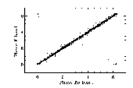
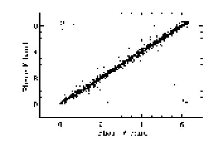
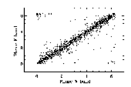
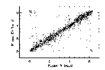
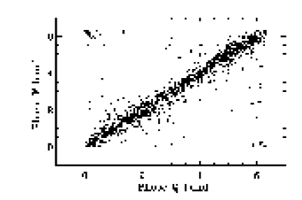
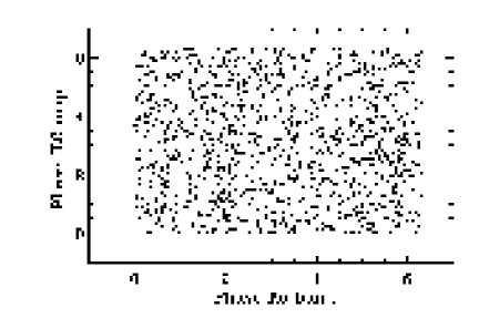
Figure 1: The cross correlations of phases between all foreground maps for the K–W bands. The phases are from all harmonic modes $\ell\leq 50$. All the foreground maps are taken from the WMAP website. Note also that on the bottom right panel we show the phases of the WMAP ILC map and the foreground map at the Ka band, which displays no correlations.

In Fig. 2 we show the phase difference between the same $\ell,m$ modes but for different K–W foreground maps, e.g. $\Psi^{{\rm Ka},f}_{\ell m}-\Psi^{{\rm K},f}_{\ell m}$ against $\Psi^{{\rm Ka},f}_{\ell m}$. One can see that the phase differences for Ka–Q band and Q–V bands are minimal, unlike, for example, for Ka–W bands. For comparison, in Fig. 3 we plot the cross correlations of phases for the total phases between the bands. As one can see from Fig. 1 and Fig. 3, all the properties of the foregrounds phases correlations manifest themselves in the cross correlation diagrams of the phases.

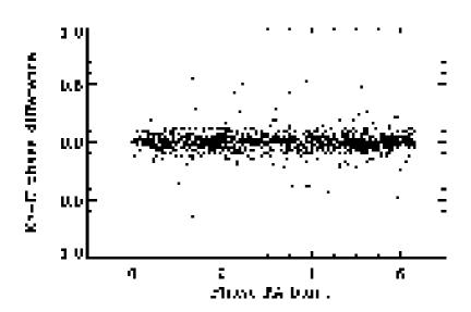
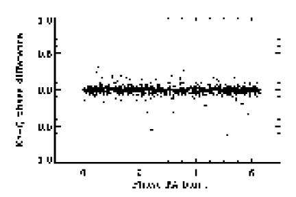
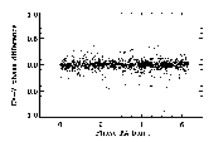
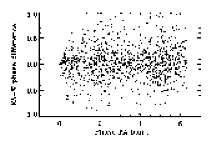
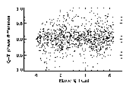
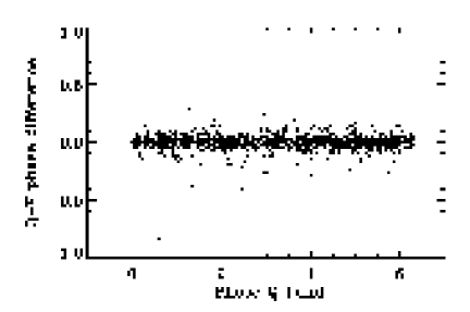
Figure 2: The phase difference at the same $\ell,m$ modes for different K–W foregrounds maps, e.g. $\Psi^{{\rm Ka},f}_{\ell m}-\Psi^{{\rm K},f}_{\ell m}$ against $\Psi^{{\rm Ka},f}_{\ell m}$ for the top left panel.

In practice, we use the Healpix package (Górski, Hivon & Wandelt, 1999) to decompose each of the WMAP K–W maps for the coefficients of spherical harmonics ${\bf a}^{(j)}$, where ${\bf a}\equiv a_{\ell m}$ and hereafter the superscript index $j=1,2,3,4,5$ correspond to the K, Ka, Q, V, W bands, respectively, after which we use the Glesp pixelization scheme (Doroshkevich et al., 2003) for the rest of data processing in order to control the accuracy of the ${\bf a}^{(j)}$ harmonics. We obtain the phases ${\bf\Psi}^{(j)}\equiv\Psi^{(j)}_{\ell m}$ from all ${\bf a}^{(j)}$ (see Eq. (2)-(4)). Each set of the ${\bf a}^{(j)}$ coefficients has the combination of different kinds of the foregrounds ${\bf a}^{(j),f}_{k}$ (convolved with the beam), the CMB signal ${\bf a}^{cmb}$ (also convolved with the beam), and the instrumental noise ${\bf n}^{(j)}$:

$${\bf a}^{(j)}=\sum_{k}{\bf a}^{(j),f}_{k}+{\bf a}^{cmb}+{\bf n}^{(j)}\equiv{\bf G}^{(j)}+{\bf a}^{cmb},$$ (5)

where $\sum_{k}{\bf a}^{(j),f}_{k}+{\bf n}^{(j)}\equiv{\bf G}^{(j)}$ is the common signal excluding the CMB at the $j$-th band. Unlike the linearity in Eq.(5), the phases of the $j$-th band are related to the phases of each kind of the foregrounds, the CMB and the instrumental noise in a non-linear manner:

$${\bf\Psi}^{(j)}=\tan^{-1}\frac{|{\bf G}^{(j)}|\sin{{\bf\Xi}^{(j)}}+|{\bf a}^{cmb}|\sin{{\bf\xi}}}{|{\bf G}^{(j)}|\cos{{\bf\Xi}^{(j)}}+|{\bf a}^{cmb}|\cos{{\bf\xi}}},$$ (6)

where ${\bf\xi}$ denotes the phases of the CMB signal and

$$|{\bf G}^{(j)}|^{2} =\sum_{k,q}\left[|{\bf a}^{(j),f}_{k}||{\bf a}^{(j),f}_{q}|\cos({\bf\Psi}^{(j),f}_{k}-{\bf\Psi}^{(j),f}_{q})\right]+$$ (7)

$$|{\bf n}^{(j)}|^{2}+2\sum_{k}|{\bf a}^{(j),f}_{k}||{\bf n}^{(j)}|\cos({\bf\Psi}^{(j),f}_{k}-{\bf\Phi}^{(j)}),$$

where ${\bf\Psi}^{(j),f}_{q}$ denotes the phases of the $q$-th foreground component at the $j$-th band and ${\bf\Phi}^{(j)}$ the phases of the noise. The phases of the common signal excluding the CMB for the $j$-th band can be written as

$${\bf\Xi}^{(j)}=\tan^{-1}\frac{\sum_{k}|{\bf a}^{(j),f}_{k}|\sin{{\bf\Psi}^{(j),f}_{k}}+|{\bf n}^{(j)}|\sin{{\bf\Phi}}^{(j)}}{\sum_{k}|{\bf a}^{(j),f}_{k}|\cos{{\bf\Psi}^{(j),f}_{k}}+|{\bf n}^{(j)}|\cos{{\bf\Phi}^{(j)}}}.$$ (8)

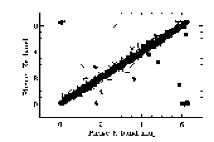
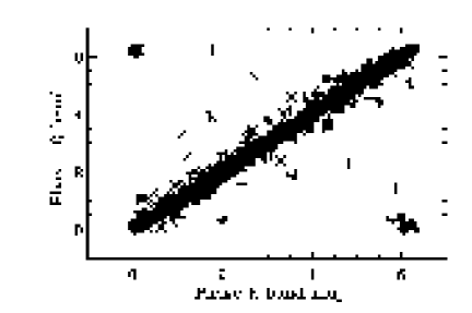
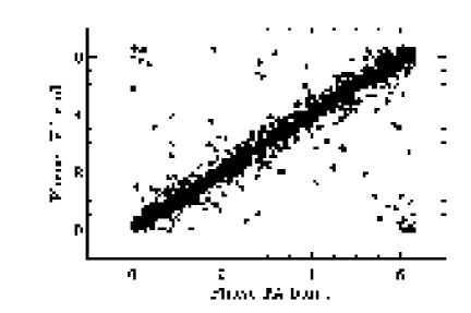
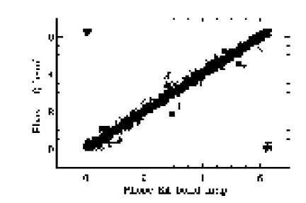
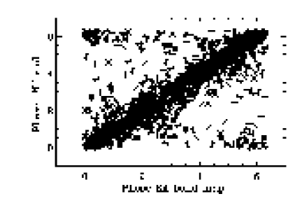
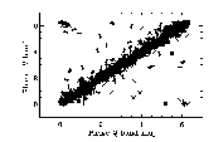
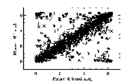
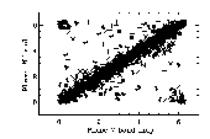
Figure 3: The cross correlations of the phases between the maps of the K–W bands.

As one can see from Eq.(7) and (8), the first term on the right hand side of Eq.(7) corresponds to the interference at the same multipoles $\ell,m$ between different foreground components, whereas the second and the third correspond to between the noise–noise and between the foreground component–noise interferences at the same frequency band, respectively. We would like to point out that these interferences can be described in terms of the auto– and cross–correlations at the same channel. However, because there is only one single realization for each frequency band these correlations are not well–established. It would be difficult to say, for example, that the instrumental noise does not correlate with the foregrounds tails by using only the 5 channels and the corresponding 5 values for each $\ell,m$ harmonic.

In our phase analysis, therefore, we use some preliminary information about the possible values of the foreground and noise amplitudes at different multipole range. That is, we discuss the properties of the signals only at the range $\ell\leq 50$, so that we can avoid the beam shape and noise properties for all the K–W bands. This multipole range is also the available range for the preliminary foreground maps on the WMAP website. Moreover, we can assume that the contribution from the instrumental noise at this range is relatively small in comparison with the synchrotron, free-free and dust emissions (except for the K band). Generally speaking, we are investigating the properties of the CMB signal at the WMAP K–W bands at the multipole range comparable with the COBE range but slightly higher. At this range the contamination of the foregrounds is the major part of the signal, including the Galactic plane.

3 The “Non-blind” Phase–Cleaned Map (PCM)

Note that we can neglect the instrumental noise and the beam shape properties when we consider multipole range $\ell\leq 50$. It is obvious that if the foreground signals are known, the pre-CMB signal can be obtained from a simple subtraction of each band map by the corresponding foreground map. We call such derived map the pre-CMB signal because we assume that the foreground signals do not have the required accuracy. As a result some residues from the foregrounds propagate to the CMB signal. In reality, all properties of the foregrounds and the pre-CMB signal come from the same combination of the K–W maps and an uncertainties of the foreground and the CMB signal estimation depend on each other. From a practical point of view, therefore, any “blind” methods would be applicable in order to find the correct phases of the CMB signal without any additional assumption about the statistical properties of the foregrounds (Tegmark & Efstathiou, 1996; Tegmark, de Oliveira-Costa & Hamilton, 2003, for example). To make the first step for finding a “blind” method for the CMB reconstruction from the phases, we consider first a “non-blind” method and will suggest a simple phase filter, the modification of which allows us to reconstruct the pre-CMB phases by a combination of the $a_{\ell m}$ coefficients of the initial CMB + foregrounds maps. This method generalizes the method from Tegmark & Efstathiou (1996), and the TOH approach, but in our case we require the minimal variance in the phases rather than in the derived map.

We use all pairs of the WMAP maps for the reconstruction of the pre-CMB maps. Below we use the pair of maps $j=1,2$ (corresponding to the maps of the WMAP K and Ka bands) as an example to derive the weighting coefficients, it can nevertheless be applied to pairs such as $j=2,3$ (Ka,Q), $2,4$ (Ka,V) and $3,4$ (Q,V). We expect to obtain the derived map $M$ from the pairs of the WMAP bands $M^{(1)}$ and $M^{(2)}$ maps, whose spherical harmonic coefficients are $a^{(1)}_{\ell m}$ and $a^{(2)}_{\ell m}$, respectively. We have

$$a^{M}_{\ell m}=\sum_{j=1}^{2}(-1)^{j+1}w^{(j)}_{\ell m}a^{(j)}_{\ell m}\equiv\sum_{j=1}^{2}(-1)^{j+1}{\bf w}^{(j)}{\bf a}^{(j)},$$ (9)

with the normalization of the filter

$$\sum_{j=1,2}(-1)^{j+1}w^{(j)}_{\ell m}={\bf I}.$$ (10)

Let us denote ${\bf w}^{(j)}=|{\bf w}^{(j)}|\exp(-i{\bf\Omega}^{(j)})$ where $|{\bf w}^{(j)}|$ and ${\bf\Omega}^{(j)}$ are the moduli and the phases of the weighting coefficients for the $j$-th band, respectively. Because of the normalization $\sum_{j}(-1)^{j+1}{\bf w}^{(j)}={\bf I}$ the moduli and phases of the filter ${\bf w}^{(j)}$ are not independent

$$|{\bf w}^{(1)}| = \frac{\sin{\bf\Omega}^{(2)}}{\sin({\bf\Omega}^{(2)}-{\bf\Omega}^{(1)})},$$

$$|{\bf w}^{(2)}| = \frac{\sin{\bf\Omega}^{(1)}}{\sin({\bf\Omega}^{(2)}-{\bf\Omega}^{(1)})},$$ (11)

and the resultant phases of the derived map $M$ are

$${\bf\Psi}^{M}=\tan^{-1}$$ (12)

$$\left(\frac{\sum_{j}(-1)^{j+1}|{\bf w}^{(j)}||{\bf G}^{(j)}|\sin({\bf\Psi}^{(j)}-{\bf\Omega}^{(j)})+|{\bf a}^{cmb}|\sin{{\bf\xi}}}{\sum_{j}(-1)^{j+1}|{\bf w}^{(j)}||{\bf G}^{(j)}|\cos({\bf\Psi}^{(j)}-{\bf\Omega}^{(j)})+|{\bf a}^{cmb}|\cos{{\bf\xi}}}\right),$$

where ${\bf G}^{(j)}$ is the common signals excluding the CMB at the $j$-th band and ${\bf\Psi}^{(j)}$ is the phases of the $j$-th band. Thus, if we prescribe that the reconstructed phase ${\bf\Psi}^{M}$ from the weighting coefficients is that of the pre-CMB signal (i.e. ${\bf\Psi}^{M}={\bf\xi}$), we reach an exact solution for the moduli and phases for the weighting coefficients

$$|{\bf w}^{(1)}| = \frac{|{\bf G}^{(2)}|}{|{\bf G}^{(1)}-{\bf G}^{(2)}|},$$

$$|{\bf w}^{(2)}| = \frac{|{\bf G}^{(1)}|}{|{\bf G}^{(1)}-{\bf G}^{(2)}|},$$

$$\sin{\bf\Omega}^{(1)} = |{\bf w}^{(2)}|\sin\Delta,$$

$$\sin{\bf\Omega}^{(2)} = |{\bf w}^{(1)}|\sin\Delta,$$ (13)

where $\Delta={\bf\Omega}^{(2)}-{\bf\Omega}^{(1)}={\bf\Psi}^{(2)}-{\bf\Psi}^{(1)}$.

Using the provided foreground maps from the WMAP database and their 5 maps for the whole signal we are able to reconstruct the pre-CMB signal using the filter Eq.(13). In Fig.3 we plot the reconstructed images of the pre-CMB signal which contain some residues. For drawing all maps we use $\ell\leq 50$ only. The top panel is a simple subtraction of the V band map by the foreground map in the V band. The middle map was obtained using the filter Eq.(13) and the pair of the WMAP Q and V maps and the their foreground maps for determination ${\bf G}^{(j)}$ and $\Delta$ in the filter Eq.(13). The bottom panel is the difference between the first two panels.

As one can see from Fig. 3 the derived pre-CMB maps look very similar, while the contaminations from the bright point-like source and diffuse residues exist notably along and perpendicular to the Galactic plane, respectively. In order to compare our derived PCM and the WMAP maps we plot the power spectrum of the 3 maps in Fig.3, using a simple pseudo-$C_{\ell}$ estimator (Hivon et al., 2002),

$$C_{\ell}=\frac{1}{2\ell+1}\sum_{m=-\ell}^{\ell}|a_{\ell m}|^{2}.$$ (14)

Note that our PCM has smaller power for the whole range of the multipoles in comparison with that derived from the V band map. The flatness of the power spectrum at $\ell>20$ clearly demonstrates the contamination of the bright point-like source residues mainly concentrated along the Galactic plane.

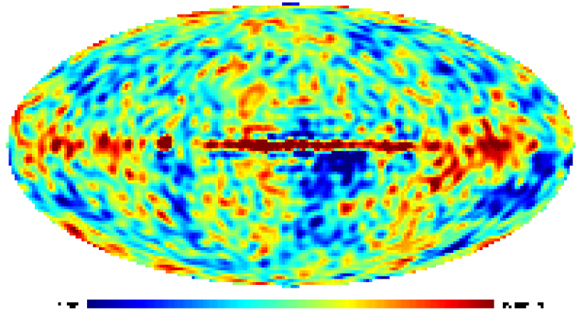
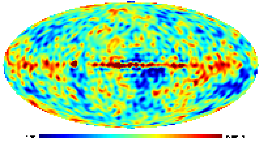
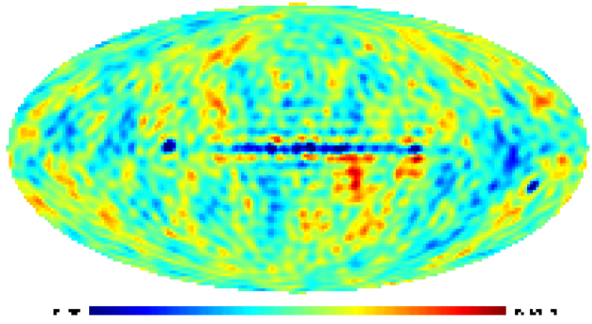
Figure 4: The maps for the derived pre-CMB signals. Top panel is the map taken from a direct subtraction of the foreground in V band by the WMAP total signal in V band. The middle panel is the cleaned-up map obtained from the “non-blind” PCM method from the WMAP Q and V bands, and the bottom the difference between the first two panels.

Figure 5: The power spectrum for the derived from the WMAP V band map (the dash dotted line), the PCM (the solid line) and the difference between the two maps (the dash line).

4 The “Blind” reconstruction of the CMB

In this section we describe the “blind” PCM method for separation of the CMB signal from the foregrounds using the K–W band signals at the harmonic range $\ell\leq 50$, avoiding again the beam convolution and the instrumental noise in Eq.(5)-(8). The main assumption is that in the different frequency bands the phases of the foregrounds do not correlate with those of the true CMB signal. The result of separation improves if there are strong correlations between the phases of the maps between the compared frequency bands (see Fig. 2).

The basic idea of the “blind” PCM method is to generalize the minimization scheme by TOH and Tegmark & Efstathiou (1996), including the minimization of the cross-correlations between derived CMB signal and foregrounds phases. This “blind” method consists the following four steps and does not need any galactic cut-offs and dissection of the whole sky into disjoint regions.

a. We firstly group the following combinations of the WMAP maps: Ka–Q, Ka–V and Q–V. They are grouped due to highly correlated phases between the bands shown in Fig. 2. We did not include the pair of the W and K bands in the separation procedure because of the reasons mentioned in Appendix B.

b. For each pair of the maps (Ka–Q, Ka–V and Q–V) we want to reach the pre-CMB map $a_{\ell m}^{M}\equiv c_{\ell m}$ derived from the pair of the bands. For Ka and Q ($j=2,3$), for example, we set $M^{(2)}\equiv a_{\ell m}^{(2)}$ and $M^{(3)}\equiv a_{\ell m}^{(3)}$ and use optimization coefficients ${{\bf\Gamma}}^{(j)}\equiv\Gamma_{\ell}^{(j)}$, similar to the TOH and Tegmark & Efstathiou (1996):

$$c_{\ell m}=\sum_{j=2}^{3}\Gamma_{\ell}^{(j)}a_{\ell m}^{(j)}\equiv\sum_{j=2}^{3}{{\bf\Gamma}}^{(j)}{\bf a}^{(j)}$$ (15)

The ${\bf\Gamma}^{(j)}$ coefficients are subject to the following constraints

$$\frac{\delta\sum_{m}|c_{\ell m}|^{2}}{\delta{\bf\Gamma}^{(j)}} = 0,$$

$$\sum_{j}{\bf\Gamma}^{(j)} = {\bf I},$$ (16)

where $\delta/\delta{\bf\Gamma}^{(j)}$ are functional derivatives. The ${\bf\Gamma}^{(j)}$ then have the following forms

$${\bf\Gamma}^{(2)} =\frac{\sum_{m}\left\{|{\bf a}^{(3)}|\left[\,|{\bf a}^{(3)}|-|{\bf a}^{(2)}|\cos({\bf\Psi}^{(3)}-{\bf\Psi}^{(2)})\,\right]\right\}}{\sum_{m}|{\bf a}^{(2)}-{\bf a}^{(3)}|^{2}},$$

$${\bf\Gamma}^{(3)} =\frac{\sum_{m}\left\{|{\bf a}^{(2)}|\left[\,|{\bf a}^{(2)}|-|{\bf a}^{(3)}|\cos({\bf\Psi}^{(3)}-{\bf\Psi}^{(2)})\,\right]\right\}}{\sum_{m}|{\bf a}^{(2)}-{\bf a}^{(3)}|^{2}}$$ (17)

where ${\bf\Psi}^{(j)}$ are the phases of the total signal at $M^{(j)}$ map. After the pre-CMB separation, we obtain the pre-CMB signal $c_{\ell m}$ and the pre-foreground at each bands.

c. The next step is to find the filter ${\bf g}^{(j)}$ to improve the foreground separation using the phase variance minimization. We will use the filter ${\bf g}^{(j)}$ in Eq.(19), which minimizes the phase difference between reconstructed and the CMB phases. We assume that ${\bf g}^{(j)}$ does not possess any imaginary part and depends only on $\ell$ but not on $m$. The theoretical basis of our choice of the form of the filter is for minimization of the weighting phase variance

$$\mbox{\~{V}}=\frac{1}{2\pi(2\ell+1)}\sum\limits_{m}\frac{|a_{\ell m}^{cmb}|^{2}}{C_{\ell}}({\bf\Psi}-{\bf\xi})^{2}\rightarrow\min$$ (18)

This condition is equivalent to minimization of the error $\varepsilon=(2\ell+1)^{-1}\sum_{m}|a_{\ell m}^{M}-a_{\ell m}^{cmb}|^{2}$ between reconstructed ($a_{\ell m}^{M}$) and the true ($a_{\ell m}^{cmb}$) CMB signals. Using foregrounds estimator ${\bf G}^{i}={\bf a}^{i}-{\bf a}^{M}$ from the step b, we obtain the following filter ${\bf g}^{(j)}$ instead of the filter (13).

$${\bf g}^{(2)} =\frac{\sum_{m}|{\bf G}^{(3)}|\left[\,|{\bf G}^{(3)}|-|{\bf G}^{(2)}|\cos({\bf\Psi}^{(3),f}-{\bf\Psi}^{(2),f})\,\right]}{\sum_{m}|{\bf G}^{(2)}-{\bf G}^{(3)}|^{2}}$$

$${\bf g}^{(3)} =\frac{\sum_{m}|{\bf G}^{(2)}|\left[\,|{\bf G}^{(2)}|-|{\bf G}^{(3)}|\cos({\bf\Psi}^{(3),f}-{\bf\Psi}^{(2),f})\,\right]}{\sum_{m}|{\bf G}^{(2)}-{\bf G}^{(3)}|^{2}}$$ (19)

where ${\bf\Psi}^{(j),f}$ are the phases of the foregrounds at the $j$-th band. This filter provides a new estimation of the foregrounds and the pre-CMB signals which we shall use for the next step of the subsequent iterations by the filter Eq.(19). So, at each iteration we insert the foreground moduli and phases obtained from the previous iteration to the same form of the filter Eq.(19). In general, 3 such iterations are enough to produce a convergent map.

d. We use a MIN-MAX filter to further clean up the residues. After the step ${\bf c.}$ we have three cleaned-up maps from the WMAP map pairs: Q–V, Ka–V and Ka–Q bands. These 3 maps correspond to the minima of the phase difference (see Fig.2). They nevertheless still contain some of the foreground residues, notably along the Galactic plane. In order to detect and minimize such a residues we used a MIN-MAX filter on the same pixel among the 3 cleaned-up maps. The definition of the MIN-MAX filter is the following. Using maps with the same pixelization scheme, we can designate all the pixels in the same way and compare simultaneously at the same pixel $p$ these 3 cleaned-up maps $\Delta T^{(i)}_{p}$ by pairing them up, where the index corresponds to the 3 cleaned-up maps. The MIN filter $L_{\min}$ allows us to find the signal which has a minimal (absolute) amplitude at the pixel $p$, i.e. $L_{\min}(\{\Delta T^{(i)}_{p}\})\rightarrow\Delta T^{\min}_{p}$, where $|\Delta T^{\min}_{p}|=\min\{|\Delta T^{(i)}_{p}|\}$.

In other words, we take the smallest absolute amplitude at the pixel $p$ from the cleaned-up maps and attach its sign for that pixel (or even more concisely, the value which is the closest to zero) .

The reason for such a filter is clear. The signal at each pixel is a combination of the underlying CMB signal and a small residue from the foreground cleaning. If the derived CMB signal correlates little with the foregrounds, it is natural to expect that all deviations of the $\Delta T^{(i)}_{p}$ at $p$ of the different maps are caused by the residues but not by the CMB. In addition to the $L_{\min}$ filter we can define a MAX filter, $L_{\max}(\{\Delta T^{(i)}_{p}\})\rightarrow\Delta T^{\max}_{p}$ which is the farthest value from zero between the maps at pixel $p$. This MAX filter reproduces the most possible contribution from the foreground residues at each pixel. Thus, we find our final PCM, the true CMB map according to the criterion that $\Delta T^{\max}_{p}-\Delta T^{\min}_{p}$ map has the mininum power. We apply our MIN-MAX filter on Q–V, Ka–V and Ka–Q cleaned-up maps and obtain the PCM signal from Q–V, Ka–V maps combination.

At the end of this Section we note the following comment. In Appendix C we show analytically that if the phase ${\bf\xi}$ of some $a_{\ell m}$ of the CMB signal is close to $\pi/2$ or $3\pi/2$ the error of the phase reconstruction is very high. Practically these phases can not be reconstructed. We call this problem the “$\pi/2$” problem. Our numerical tests (see section 5) confirm this conclusion.

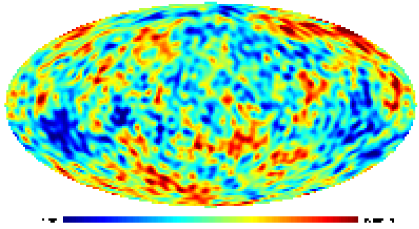
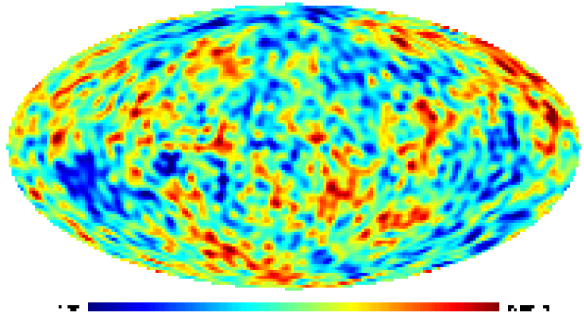
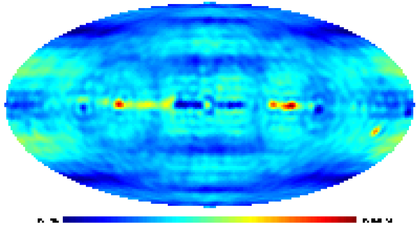
Figure 6: The reconstructed PCM from the wmap simulator. Top panel is the simulated CMB map and the middle is the reconstructed PCM from the two pairs of simulated bands, Q–V and Ka–V. The bottom panel is the difference between the two.

5 The numerical test

To numerically test the “blind” PCM method we use a wmap simulator to mimic all the properties of the WMAP foregrounds at K-W bands. We again exclude the instrumental noise and the beam shape properties, which are insignificant for the multipole range $\ell\leq 50$. We take the best-fit WMAP $\Lambda$CDM power spectrum to produce a simulated CMB sky with random phases. Such CMB sky is truly a Gaussian random realization. The morphology of this simulated CMB map is obviously different from that of the WMAP ILC and the TOH maps (since it has a different set of random phases). For our wmap simulator we adopt all the foreground maps for each frequency band from the WMAP website. We also confirm that the simulated CMB signal does not have any cross-correlation with the foregrounds and it has well-defined statistical properties (the power spectrum and random phases).

Figure 7: The reconstructed power spectrum of the wmap simulator from the “blind” PCM method. The solid line is the power spectrum of the simulated CMB signal and the dash-dot line is that of the reconstructed PCM. Note that both curves almost overlap except for $\ell=2$, 5 and 7. The dashed line is the difference of these two. These 3 power spectra correspond to the 3 panels in Fig.4. The reconstructed PCM signal is produced from two pairs of the simulated channels, Q–V and Ka–V.

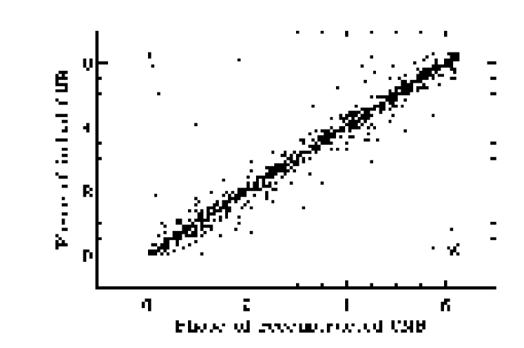
Figure 8: The cross correlation of the phases between the simulated (random-phase) CMB and the reconstructed CMB (PCM) signal. The solid diagonal line indicates an asymptotic when the simulated and reconstructed phases are identical.

In Fig.4 we show the result of the CMB reconstruction after 10 iterations from the “blind” PCM method. As we mention above the third and all subsequent iterations practically produce a convergent cleaned-up map. We take two pairs of simulated channels, Q–V and Ka–V, to reconstruct the signal. The result of reconstruction for both pairs was practically the same, and the MIN-MAX filter is used to produce the resultant reconstructed map shown in Fig.4. In Fig.5 we plot the power spectra for the simulated and the reconstructed CMB (PCM) signals as a function of $\ell$. Both curves almost overlap except for $\ell=2$, 5 and 7.

In Fig.5 we plot the cross-correlation of the phases between the simulated CMB signal and the reconstructed CMB (PCM). As one can see from Fig. 5 for reconstructed CMB signal the quadrupole component has smaller power than the simulated CMB. The reason for that is that the peculiar phases of the quadrupole component $Q_{20}$, $Q_{21}$ and $Q_{22}$. Accidentally, in our simulated realization of the CMB (see Fig.4) the phases of the component $Q_{20}$ and $Q_{21}$ are zero whereas for the $Q_{22}$ component the corresponding phase is close to $3\pi/2$ with only 10% deviation. That is why the reconstructed phase of $Q_{22}$ component has ${\bf\xi}_{22}=6.227$ radians.

In Fig.5 we plot the cross correlation of the phases between the reconstructed CMB signal (PCM) and the simulator foregrounds at all 5 simulated bands. The scattering of points in all 5 panels indicates that the phases of the PCM display no serious correlations with those of the foregrounds. The wmap simulator therefore confirms the usefulness of our “blind” PCM method for the CMB extraction without any assumptions about the statistical properties of the foregrounds.

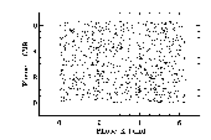
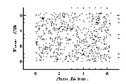
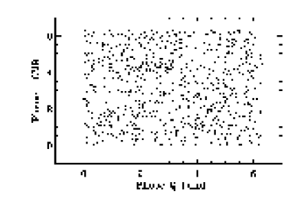
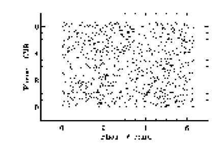
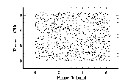
Figure 9: The cross correlations of the phases between the reconstructed CMB signal (PCM) and the simulator foregrounds of all 5 simulated bands. The scattering of points in all 5 panels indicates that the phases of the PCM display no correlations with those of the foregrounds.

6 The PCM derived from the 1-year WMAP data

For the reconstruction of the CMB signal at $\ell\leq 50$ from the K–W bands of the WMAP data we use the three pairs of the maps: Ka–Q, Q–V and Ka–V. We repeat the steps ${\bf b}$ and ${\bf c}$ of the “blind” PCM method : each of them has been convolved by the weighting coefficients, Eq.(17) and then by the coefficients Eq.(19) using only 2 iterations. All the next iterations do not change significantly the $a_{\ell m}$ coefficients (the corresponding error being less than $10^{-3}\%$). The results are present in Fig.6, in which all the 3 cleaned-up maps have pronounced similarity in morphology, albeit with some residues from the galactic foregrounds.

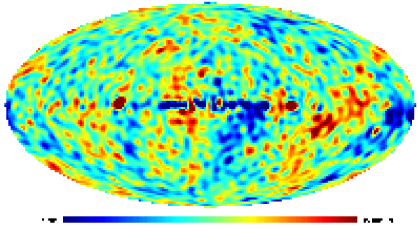
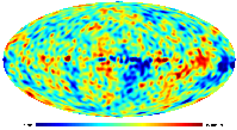
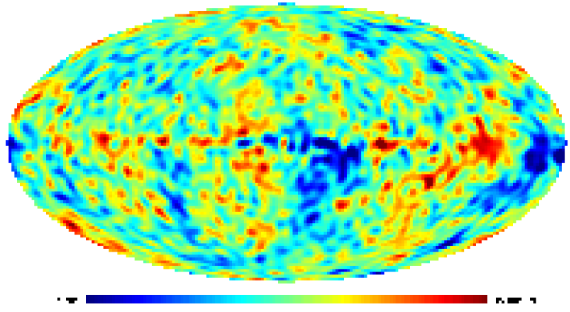
Figure 10: The cleaned-up maps after the steps ${\bf b}$ and ${\bf c}$ from the “blind” PCM method on the 3 pairs of WMAP maps. The top panel is the cleaned-up map from the Ka–Q maps, the middle the cleaned-up map from the Ka–V maps, and the bottom from the Q–V maps.

In Fig.6 we show the result after the step ${\bf d}$, the MIN-MAX filtering. The top panel is our CMB signal (the PCM), the middle is the WMAP ILC map for comparison and the bottom is the difference of the two.

In Fig.6 we plot the CMB angular power spectra from different methods: the thick solid line is the PCM, the dashed line the WMAP ILC map, the dash-dot line the TOH foreground-cleaned map, and the thin solid line the TOH Wiener-filtered map. The PCM power spectrum is smaller then ILC power spectrum at the whole multipole range $\ell\leq 50$ and it reproduces a similar power spectrum as the TOH Winer-filtered map.

In Fig.6 we show the cross correlation of the phases between the PCM and the foreground maps of the WMAP bands. Again the scattering of the points shows that the phases of the PCM practically have no correlations with those of the foregrounds.

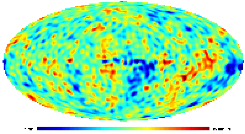
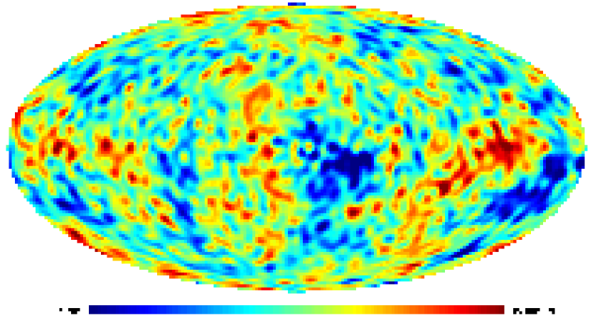
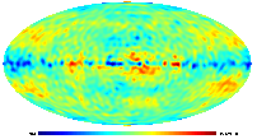
Figure 11: The CMB map (the PCM) after the step ${\bf d}$ of the “blind” PCM method (top panel). The MIN-MAX filter is performed on the 3 panels of Fig.6. For comparison, the middle is the WMAP ILC map and the bottom is the difference of the two.

Figure 12: The comparison of the CMB angular power spectra from different methods. The power spectrum of the PCM is shown with the thick solid line, that of the WMAP ILC map is shown with the dashed line, the TOH foreground-cleaned map the dash-dot line, and the TOH Wiener-filtered map the thin solid line.

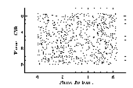
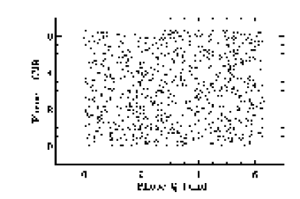
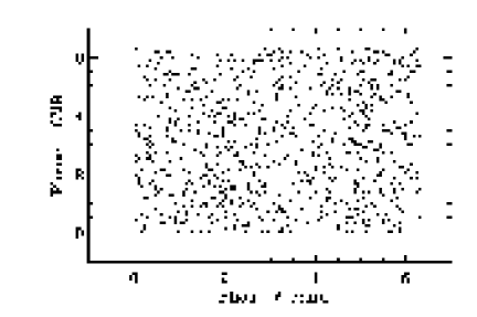
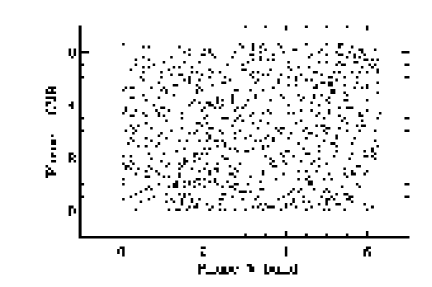
Figure 13: Cross correlation of the phases between the PCM and the WMAP foreground maps of the WMAP Ka, Q, V and W bands. Again the scattering of the points shows that the phases of the PCM practically have no correlations with those of the foregrounds.

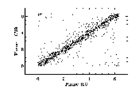
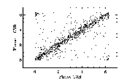
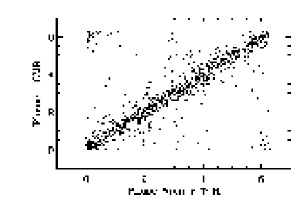
Figure 14: Cross correlation of the phases between the PCM and the WMAP ILC map (top left), between the PCM and the TOH foreground-cleaned map (top right), and between the PCM and the TOH Wiener-filtered map (bottom).

Although the phases of the PCM have strong correlations with those of the ILC map, the TOH foreground-cleaned map and the Wiener-filtered map, as shown in Fig.6, there are undoubtedly deviations in phases between them, which is an indication of different morphology.

The CMB map from the “blind” PCM method allows us to reconstruct the foregrounds for each WMAP band. In Fig.6 we show at the top the foreground map at the V band, a simple subtraction of the PCM from the WMAP V-band map. In the middle panel we show the WMAP foreground map at the same band and the difference of these two panels is shown at the bottom. As one can see from this Figure, an additional power of the foregrounds from the PCM subtraction than the WMAP foreground map is clearly shown in the third panel, in particular we can see strong contribution of the of the point-like sources residues along the Galactic plane which are detected and removed as foregrounds from the PCM subtraction.

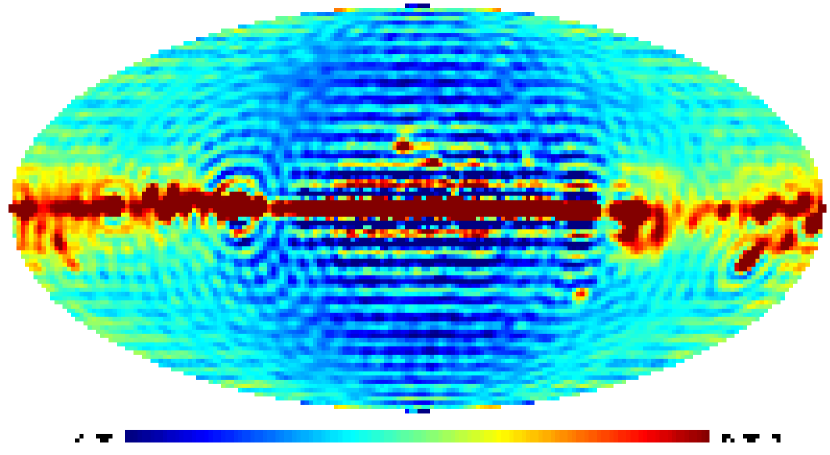
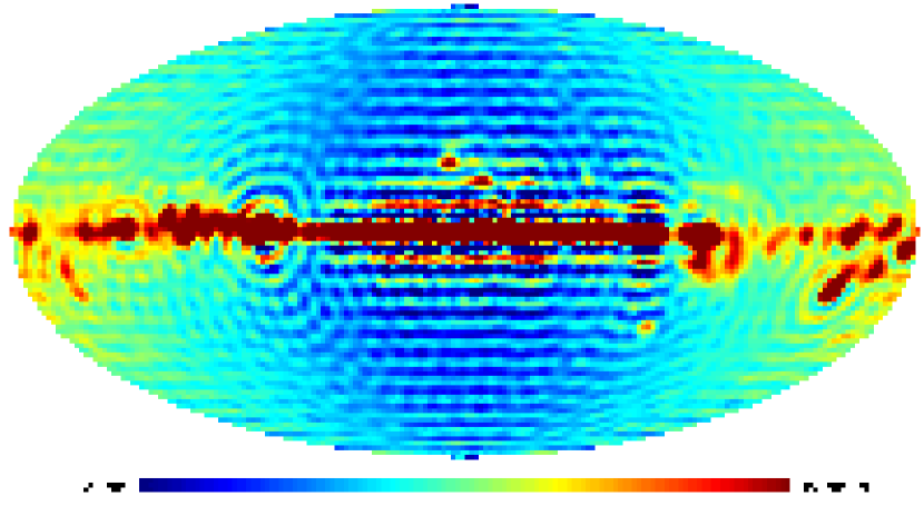
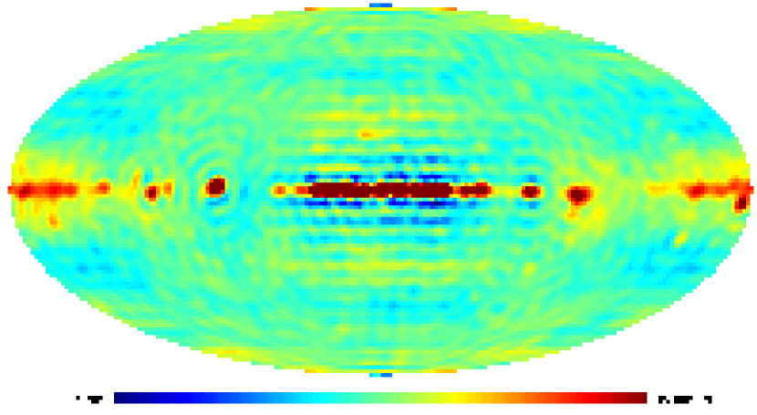
Figure 15: The foreground map at the V band from the subtraction of the PCM from the WMAP V-band map (top), the WMAP foreground map at the V band (middle) and the difference of the first two maps (bottom).

7 Non-Gaussianity testing on the PCM

In this section we use the phase mapping technique as a non-Gaussian test to compare the non-Gaussianity between the PCM, the WMAP ILC map and the TOH Wiener-filtered map. This method has been successful in detecting non-Gaussianity in the derived TOH maps from the WMAP data (Chiang, Naselsky, Verkhodanov & Way, 2003).

The null hypothesis of the phase mapping technique is based on the so-called random-phase hypothesis, which is served as a practical definition of homogeneous and isotropic Gaussian random fields (Bardeen et al., 1986). Therefore, any non-random phases from harmonic analyses is interpreted as manifestation of non-Gaussianity. Due to the circular character of phases, we use the return mapping of phases with certain separations $(\Delta m,\Delta\ell)$ to render phases on return maps. Testing random phases is thus equivalent to testing randomness of each return map. There are many ways of quantifying such ensemble of return maps. We choose the simplest $\overline{\chi^{2}}$ statistic as in Chiang, Naselsky & Coles (2002): we first use a Gaussian window function to smooth each return map and use a simple $\overline{\chi^{2}}=(1/M)\sum_{i,j}[p(i,j)-\overline{p}]^{2}/\overline{p}$ to yield the statistics, where $\overline{p}$ is the mean value and $M$ is the number of pixels. The null hypothesis will have mean $\langle\overline{\chi^{2}}\rangle_{\rm P}=1/4\pi R^{2}$ and dispersion $\Sigma_{\rm P}^{2}=1/\pi^{3}R^{2}(M/2)$.

We perform the mean $\chi^{2}$ statistics derived from phase mapping technique for the PCM, the ILC map and the TOH Wiener-filtered map. We take the phases from $\ell=2$ to maximum $\ell=40$ and render 256 points on each return map. The smoothing scale of the Gaussian window function is $R=1$. The ensemble of return maps consists of separation $\Delta m$ from $-9$ to 20 and $\Delta\ell$ from 1 to 15. From the distribution function of such ensemble, we use the mean $\langle\overline{\chi^{2}}\rangle$ and the dispersion $\Sigma$ of the distribution function as two independent variables for displaying the statistics. We simulate 2000 realizations of Gaussian random fields to yields reliability. In Fig. 7 the dashed and dotted contours indicate 68%, 95% confidence level for detection, respectively. The non-Gaussianity through phase mapping test shows that the PCM and the Wiener-filtered map have close non-Gaussianity, whereas the WMAP ILC map shows less non-Gaussian. Note that, however, both the ILC map and Wiener-filtered map are produced by dissecting the whole-sky CMB maps into 12 and 9 disjoint regions for cleaning, which systematically change the phase configuration for the whole sky.

Figure 16: Non-Gaussianity test using the phase mapping technique for the PCM map (cross) at multipole range $2\leq\ell\leq 40$, the WMAP ILC map (triangle) and the TOH Wiener-filtered map (box). The dashed contour corresponds to 68% CL, the dotted contour corresponds to 95% CL.

8 Discussions and conclusions

In this paper we have proposed a new method for the separation of the CMB signal from the Galactic and other foregrounds based on the phase cleaning of the WMAP K–W bands at the multipole range $\ell\leq 50$. This method is based on a simple but prevailing assumption that the phases of the CMB signal should not correlate with those of the foregrounds. We first propose a “non-blind” PCM method using the foreground maps available at the WMAP website as preliminary foregrounds. We then introduce a “blind” PCM method with 4-step foreground cleaning. We firstly group into pairs from the maps which have strong cross correlations in phase. We then in step ${\bf b}$ use a simple TOH minimization of the variance of the combination between different pairs of K–W maps. In the step ${\bf c}$ we propose a phase-cleaning filter for each derived map from the constraint of minimal variance of phase difference. Finally, we propose a MIN-MAX filter in order to obtain the PCM map. Our CMB signal (the PCM) has the power spectrum in an excellent agreement with the best fit WMAP cosmological model, but the phases are slightly different from those of the WMAP ILC map. We also confirm that, after phase cleaning, the PCM has essentially no correlation in phases with their cross-correlation with the foregrounds. We would like to point out that the PCM method can be used with different component separation methods such as the Maximum Entropy Method (MEM) or another methods, which can be used an initial step before the phase cleaning. Such generalization on the PCM method is in progress.

Using the PCM method we have found corresponding corrections of the foreground maps for each K–W band, which is useful for the data analysis for the upcoming Planck mission. The power spectra of the common foreground maps from our PCM subtraction are slightly different from the WMAP foreground maps. Moreover, the PCM does not show any serious contamination from the point-like source residues mainly thanks to the MIN-MAX filter.

The PCM CMB signal, as it follows from comparison between our CMB and WMAP maps has a power smaller then ILC map.

We also confirm that the PCM displays a low level of power at the quadrupole component, which also manifest itself in the WMAP ILC map and the TOH map (Tegmark, de Oliveira-Costa & Hamilton, 2003; de Oliveira-Costa, Tegmark, Zaldarriaga & Hamilton, 2003). However, the low level in $C_{\ell}$ is typical at the multipole range $2\leq\ell\leq 10$. In order to compare the power spectrum of the PCM with that of the WMAP best fit model and the TOH Wiener-filtered map, in Fig.8 we plot these power spectra with the error bars caused by the cosmic variance.

Figure 17: The power spectra of the PCM (the thick solid line) and the TOH Wiener-filtered map (thick dashed line). The cosmic variance error bars with 68% CL are indicated with crosses with the triple dots dashed lines.

As one can see from Fig.8 all deviations between the PCM and the TOH Wiener-filtered map are within the 68% CL. Some of the multipole range, however, seems to be quite peculiar. Namely, at $20\leq\ell\leq 24$ the power of both the PCM and the TOH Wiener-filtered map has some suppression. Does it indicate that we have a peculiar realization of a Gaussian random CMB field? Or we still have the contaminations of the foregrounds which mimic as extra CMB power? All these issues can only be discussed when more data are available, particularly the future polarization observational data.

In this paper we concentrate only on the low multipole range of the CMB $\ell\leq 50$, at which the beam shape and the instrumental noise are not crucial. The development of the PCM method and the results at the multipole range $\ell>50$ is in preparation.

Appendix A A : The concept of the “blind” PCM method

From Eq.(9) and (13), one might think that it is possible to generalize the “non-blind” phase reconstruction method to the “blind” variant simply using the $a_{\ell m}$ coefficients in Eq.(13) as an estimator for the reconstructed phases of the pre-CMB signal. Such generalization, however, would be incorrect because of the following reason. Below we consider only for the multipole range $\ell\leq 50$ to avoid the instrumental noise and beam shape properties. According to Eq.(5) the moduli of the $a_{\ell m}$ coefficients are related with the moduli of the foregrounds and CMB for each WMAP band as (with the phases ${\bf\Xi}^{(j)}$ in Eq.(5) being replaced by ${\bf\Psi}^{(j),f}$, the resultant foreground phases)

$$|{\bf a}^{(j)}|^{2}=|{\bf G}^{(j)}|^{2}+2|{\bf G}^{(j)}||{\bf a}^{cmb}|\cos({\bf\Psi}^{(j),f}-{\bf\xi})+|{\bf a}^{cmb}|^{2}$$ (A1)

where $|{\bf a}^{cmb}|\ll|{\bf G}^{(j)}|$. Using Taylor series one can obtain $|{\bf a}^{(j)}|\sim|{\bf G}^{(j)}|+|{\bf a}^{cmb}|\cos({\bf\Psi}^{(j),f}-{\bf\xi})$. Then, from Eq.(12) we get

$$\sum_{j}(-1)^{j+1}{\bf w}^{(j)}|{\bf a}^{(j)}| \sim \frac{|{\bf a}^{cmb}|}{|{\bf a}^{(1)}-{\bf a}^{(2)}|}\left[|{\bf G}^{(1)}|\cos({\bf\Psi}^{(1),f}-{\bf\xi})-|{\bf G}^{(2)}|\cos({\bf\Psi}^{(2),f}-{\bf\xi})\right]$$ (A2)

$$= \frac{|{\bf a}^{cmb}|}{|{\bf a}^{(1)}-{\bf a}^{(2)}|}\cos({\bf\Psi}^{(1),f}-{\bf\xi})\left[|{\bf G}^{(1)}|-|{\bf G}^{(2)}|\cos\Delta+|{\bf G}^{(2)}|\sin\Delta\,\tan({\bf\Psi}^{(1),f}-{\bf\xi})\right]$$

The comparison of Eq.(A2) and Eq.(12) allow us to conclude that the deviation of the reconstructed phases from the CMB phases should be very high even for the small values of $\Delta$-parameter. This means that the reconstructed phases of the CMB signal would be close to the foreground phases and the corresponding power spectrum should have very significant errors. It is important to note that such a conclusion means that in order to extract the correct phases and amplitudes of the CMB signal from the data using a “blind” method of separation, it is necessary to decrease the contamination in Eq.(A1) of the linear term ($\sim|{\bf a}^{cmb}|\cos({\bf\Psi}^{(j),f}-{\bf\xi})$). The only way to do this is to take into account that $\sum_{m}|{\bf a}^{cmb}|\cos({\bf\Psi}^{(j),f}-{\bf\xi})\rightarrow 0$ for high $\ell,m$. In such a case $\sum_{j}(-1)^{j+1}{\bf w}^{(j)}|{\bf a}^{(j)}|\sim{\cal O}(|{\bf a}^{cmb}|^{2})$ and corresponding error of the CMB phase reconstruction should be of the order $|{\bf a}^{cmb}|/\min\{|{\bf G}^{(j)}|\}$. Moreover, averaging over the $m$ values means that the corresponding weighting coefficients ${\bf w}^{(j)}$ is a function of $\ell$ only, but not of $m$, which is ideologically close to Tegmark & Efstathiou (1996) and the TOH method, where ${\bf w}^{(j)}=w^{(j)}(\ell)$. We would like to point out, however, that for such an optimization, as indicated in Eq.(12), the reconstructed CMB phases will have the cross correlations with the foregrounds phases at different levels for different modes.

Appendix B B : Minimization of the phase difference

Assuming that the reconstructed phase ${\bf\Psi}^{M}$ should be close to the CMB phase ${\bf\xi}$, from Eq.(12), we obtain

$${\bf\Psi}^{M}={\bf\xi}+\arcsin\frac{\sum_{j}{\bf g}^{(j)}|{\bf G}^{(j)}|\sin({{\bf\Psi}^{(j),f}-{\bf\xi})}\cos{\bf\Psi}^{M}}{\sum_{j}{\bf g}^{(j)}|{\bf G}^{(j)}|\cos{{\bf\Psi}^{(j),f}}+|{\bf a}^{cmb}|\cos{{\bf\xi}}}.$$ (B1)

As mentioned above, a new element of the “blind” reconstruction of the CMB signal is the correlation between the derived phases ${\bf\Psi}^{M}$ and the foreground phases ${\bf\Psi}^{(j),f}_{1},{\bf\Psi}^{(j),f}_{2}$ for all linear combinations of the maps. Moreover, if

$$|{\bf a}^{cmb}|\cos{{\bf\xi}}\gg\sum_{j}{\bf g}^{(j)}|{\bf G}^{(j)}|\cos{{\bf\Psi}^{(j),f}},$$ (B2)

then ${\bf\Psi}^{M}\simeq{\bf\xi}$ while for some of the $\ell,m$ modes which corresponds to inequality $|{\bf a}^{cmb}|\cos{{\bf\xi}}\ll\sum_{j}{\bf g}^{(j)}|{\bf G}^{(j)}|\cos{{\bf\Psi}^{(j)}}$, reconstruction of the CMB phases needs more specific investigation, which will be discussed at the end of the section. For all $\ell,m$ modes satisfying Eq.(B2) in order to decrease the correlation between the foregrounds and CMB phases we introduce the optimization scheme based on the iterative solution of the Eq.(B1). The first step of iterations is to minimize the variance

$$V=\frac{1}{2\pi}\int_{0}^{2\pi}d{\bf\xi}\left({\bf\Psi}^{M}-{\bf\xi}\right)^{2}\rightarrow\min,$$ (B3)

which corresponds to the equation

$$\frac{\delta V}{\delta{\bf g}^{(k)}}=\frac{1}{4{\pi}}\frac{\delta}{\delta{\bf g}^{(k)}}\left\{\sum_{i,j}\frac{{\bf g}^{(i)}{\bf g}^{(j)}|{\bf G}^{(j)}||{\bf G}^{(i)}|}{|{\bf a}^{cmb}|^{2}}\left[I_{1}\cos({\bf\Psi}^{(j),f}-{\bf\Psi}^{(i),f})-I_{2}\right]\right\}=0,$$ (B4)

where $\delta/\delta{\bf g}^{(k)}$ are the functional derivatives and

$$I_{1} = \int_{0}^{2\pi}d{\bf\xi}\frac{\cos^{2}{\bf\xi}}{(\cos{\bf\xi}+\beta)^{2}},$$

$$I_{2} = \int_{0}^{2\pi}d{\bf\xi}\frac{\cos^{2}{\bf\xi}\cos({\bf\Psi}^{(j),f}+{\bf\Psi}^{(i),f}-2{\bf\xi})}{(\cos{\bf\xi}+\beta)^{2}},$$ (B5)

and

$$\beta=\frac{1}{|{\bf a}^{cmb}|}\sum_{j}{\bf g}^{(j)}|{\bf G}^{(j)}|\cos{{\bf\Psi}^{(j),f}}.$$ (B6)

Note that $\beta$ could be both positive and negative depending on the phases ${{\bf\Psi}^{(j),f}}$. As we mention above, Eq.(B4) has an exact solution not for all values of $\ell,m$. For $\ell,m$ satisfying Eq.(B2) we can neglect the $\beta$ parameter in Eq.(B5) and obtain $I_{1}\simeq 2\pi$, $I_{2}\simeq 0$. Thus, from Eq.(B4)-(B6) we have

$${\bf g}^{(1)} = \frac{|{\bf G}^{(2)}|\left[|{\bf G}^{(2)}|-|{\bf G}^{(1)}|\cos({\bf\Psi}^{(2),f}-{\bf\Psi}^{(1),f})\right]}{|{\bf G}^{(1)}-{\bf G}^{(2)}|^{2}},$$

$${\bf g}^{(2)} = \frac{|{\bf G}^{(1)}|\left[|{\bf G}^{(1)}|-|{\bf G}^{(2)}|\cos({\bf\Psi}^{(2),f}-{\bf\Psi}^{(1),f})\right]}{|{\bf G}^{(1)}-{\bf G}^{(2)}|^{2}}.$$ (B7)

The filter Eq.(B7) depends on both $\ell$ and $m$. As one can see from Eq.(B7), if the phases of the foregrounds ${\bf\Psi}^{(2),f}$ and ${\bf\Psi}^{(1),f}$ are identical, then one can have the same form for the ${\bf g}^{(1)}$ and ${\bf g}^{(2)}$ weighting coefficients as in Eq.(13). Unfortunately, because of the non-zero phase difference ${\bf\Psi}^{(2),f}-{\bf\Psi}^{(1),f}$ the filter (B7) is not useful for the “blind” method of the CMB reconstruction. It is due to the instability of the iteration sheme, which reproduces at the very first step the phases of the foregrounds and use them as an attractor.

Now following the concept in Appendix A, let us introduce another concept of the phase optimization based on the minimization of the weighting phase variance

$$V=\frac{1}{2\pi(2\ell+1)}\sum_{m}\frac{|{\bf a}^{cmb}|^{2}}{C_{\ell}}\int_{0}^{2\pi}d{\bf\xi}\left({\bf\Psi}^{M}-{\bf\xi}\right)^{2}\rightarrow\min,$$ (B8)

which corresponds to the following

$$\frac{\delta V}{\delta{\bf g}^{(k)}}\propto\frac{\delta}{\delta{\bf g}^{(k)}}\left[\sum_{m}\sum_{i,j}{\bf g}^{(i)}{\bf g}^{(j)}|{\bf G}^{(j)}||{\bf G}^{(i)}|\cos({\bf\Psi}^{(j),f}-{\bf\Psi}^{(i),f})\right]=0,$$ (B9)

and

$${\bf g}^{(1)} = \frac{\sum_{m}|{\bf G}^{(2)}|\left[\,|{\bf G}^{(2)}|-|{\bf G}^{(1)}|\cos({\bf\Psi}^{(2),f}-{\bf\Psi}^{(1),f})\,\right]}{\sum_{m}|{\bf G}^{(1)}-{\bf G}^{(2)}|^{2}},$$

$${\bf g}^{(2)} = \frac{\sum_{m}|{\bf G}^{(1)}|\left[\,|{\bf G}^{(1)}|-|{\bf G}^{(2)}|\cos({\bf\Psi}^{(2),f}-{\bf\Psi}^{(1),f})\,\right]}{\sum_{m}|{\bf G}^{(1)}-{\bf G}^{(2)}|^{2}}.$$ (B10)

It is easy to demonstrate that the filter Eq.(B10) corresponds to the minimum of the variance $\sum_{m}|{\bf a}^{M}-{\bf a}^{cmb}|^{2}$. We propose to use this filter for optimization of the pre-CMB reconstruction at the second and subsequent iterations.

Appendix C C : The “$\pi/2$” problem of the phases reconstruction

In this Appendix we discuss some problems of the CMB image reconstruction related with optimization methods. The exact solution for the reconstructed phases in a form of Eq.(B10) has some peculiar reconstructed phases ${\bf\Psi}^{M}$ if the CMB phases ${\bf\xi}$ are close to $\pi/2$ and $3\pi/2$. In such a case, from Eq.(B4) we obtain

$${\bf\Psi}^{M}\simeq\tan^{-1}\left(\frac{|a^{cmb}|\cos\delta}{\sum_{j}{\bf g}^{(j)}|{\bf G}^{(j)}|\cos{{\bf\Psi}^{(j),f}}}+\frac{\sum_{j}{\bf g}^{(j)}|{\bf G}^{(j)}|\sin{{\bf\Psi}^{(j),f}}}{\sum_{j}{\bf g}^{(j)}|{\bf G}^{(j)}|\cos{{\bf\Psi}^{(j),f}}}\right),$$ (C1)

where ${\bf\xi}=\pi/2+\delta$, $\delta\ll 1$ and $|a^{cmb}|\cos{\bf\xi}\ll\sum_{j}{\bf g}^{(j)}|{\bf G}^{(j)}|\cos{{\bf\Psi}^{(j),f}}$. We point out that depending on the foreground phases the reconstructed phase ${\bf\Psi}^{M}$ could be arbitrary. It means that phases close to $\pi/2$ will be reconstructed with a big error. The same argument can be applied to the case when ${\bf\xi}$ is close to $3\pi/2$.

References

- (1)
- (2)
- (3)
- (4)
- (5)
- (6)
- (7)
- (8)
- Bardeen et al. (1986) Bardeen, J.M., Bond, J.R., Kaiser, N., Szalay, A.S., 1986, ApJ, 304, 15
- Barreiro et al. (2003) Barreiro, R. B., Hobson, M. P., Banday, A. J., Lasenby, A. N., Stolyarov, V., Vielva, P., Górski, K. M., 2003, MNRAS submitted (astro-ph/0302091)
- Bennett et al. (2003a) Bennett, C. L., et al., 2003, ApJ, 583, 1
- Bennett et al. (2003b) Bennett, C. L., et al., 2003, ApJS, 148, 1
- Bennett et al. (2003c) Bennett, C. L., et al., 2003, ApJS, 148, 97
- Bouchet & Gispert (1999) Bouchet, F. R., Gispert, R., 1999, New Astronomy, 4, 443
- Chiang (2001) Chiang, L.-Y., 2001, MNRAS, 325, 405
- Chiang & Coles (2000) Chiang, L.-Y., Coles, P., 2000, MNRAS, 311, 809
- Chiang, Coles & Naselsky (2002) Chiang, L.-Y., Coles, P., Naselsky, P. D., 2002, MNRAS, 337, 488
- Chiang, Naselsky & Coles (2002) Chiang, L.-Y., Naselsky, P. D., Coles, P., 2002, ApJL submitted (astro-ph/0208235)
- Chiang, Naselsky, Verkhodanov & Way (2003) Chiang, L.-Y., Naselsky, P. D., Verkhodanov, O. V., Way, M. J., 2003, ApJL, 590, 65
- Delabrouille, Patanchon & Audit (2003) Delabrouille, J., Patanchon, G., Audit, E., 2002, MNRAS, 330, 807
- de Oliveira-Costa, Tegmark, Zaldarriaga & Hamilton (2003) de Oliveira-Costa, A., Tegmark, M., Zaldarriaga, M., Hamilton, A., 2003, Phys. Rev. D accepted (astro-ph/0307282)
- Doroshkevich et al. (2003) Doroshkevich, A. G., Naselsky, P. D., Verkhodanov, O. V., Novikov, D. I., Turchaninov, V. I., Novikov, I. D., Christensen, P. R., 2003, A&A submitted (astro-ph/0305537)
- Efstathiou (2003) Efstathiou, G., 2003, MNRAS submitted (astro-ph/0306431)
- Eriksen et al. (2003) Eriksen, H. K., Hansen, F. K., Banday, A. J., Górski, K. M., Lilje, P. B., 2003, ApJL submitted (astro-ph/0307507)
- Górski, Hivon & Wandelt (1999) Górski, K. M., Hivon, E., Wandelt, B. D., 1999, Proceedings of the MPA/ESO Cosmology Conference “Evolution of Large-Scale Structure”, eds. A. J. Banday, R. S. Sheth and L. Da Costa, PrintPartners Ipskamp, NL, ,
- Hinshaw et al. (2003a) Hinshaw, G., et al., 2003, ApJS, 148, 63
- Hinshaw et al. (2003b) Hinshaw, G., et al., 2003, ApJS, 148, 135
- Hivon et al. (2002) Hivon, E., Gorski, K. M., Netterfield, C. B., Crill, B. P., Prunet, S., Hansen, F., 2002, ApJ, 567, 2
- Hobson et al. (1998) Hobson, M. P., Jones, A. W., Lasenby, A. N., Bouchet, F. R., 1998, MNRAS, 300, 1
- Komatsu et al. (2003) Komatsu, E., et al., 2003, ApJS, 148, 119
- Martinez-Gonzalez et al. (2003) Martinez–Gonzalez, E., Diego, J. M., Vielva, P., Silk, J., 2003, MNRAS accepted (astro-ph/0302094)
- Naselsky, Novikov & Silk (2002) Naselsky, P. D., Novikov, D. I., Silk, J., 2002, MNRAS, 335, 550
- Park (2003) Park, C.-G., 2003, MNRAS submitted (astro-ph/0307469)
- Patanchon et al. (2003) Patanchon, G., Snoussi, H., Cardoso, J. F., Delabrouille, J., 2003, PSIP03 conference Grenoble (astro-ph/0302078)
- Stolyarov et al. (2002) Stolyarov, V., Hobson, M. P., Ashdown, M. A. J., Lasenby, A. N., 2002, MNRAS, 336, 97
- Tegmark & Efstathiou (1996) Tegmark, M., Efstathiou, G., 1996, MNRAS, 281, 1297
- Tegmark, de Oliveira-Costa & Hamilton (2003) Tegmark, M., de Oliveira-Costa, A., Hamilton, A., 2003, Phys. Rev. D accepted (astro-ph/0302496)