Determination of the calorimetric energy in extensive air showers

Abstract

The contribution of different components of an air shower to the total energy deposit in the atmosphere, for different angles and primary particles, was studied using the CORSIKA air shower simulation code. The amount of missing energy, parameterized in terms of the calorimetric energy, was calculated. The results show that this parameterization varies less than $1\%$ with angle or observation level. The dependence with the primary mass is less than $5\%$ and, with the high energy hadronic interaction model, less than $2\%$. The systematic error introduced by the use of just one parameterization of the missing energy correction function, for an equal mixture of proton and iron at $45^{o}$, was calculated to be below $3\%$. We estimate the statistical error due to shower-to-shower fluctuations to be about $1\%$.

, , and

1 Introduction

In the last years, the quest to unravel the many mysteries related to the cosmic radiation has been intensified, in an attempt to answer open questions [1, 2] about origin, propagation and chemical composition of the ultra high energy cosmic rays. The Auger [3] observatory, now under construction, and future experiments like Telescope Array [4], EUSO [5] and OWL [6] will shed light on these questions.

A common feature of these experiments is the use of the fluorescence technique, first explored by the Fly’s Eye group [7]. The fluorescence telescopes use the atmosphere as a calorimeter, making a direct measurement of the longitudinal shower development, which represents the most appropriate technique to determine the energy of the primary particle. This is based on the assumption that the fluorescence yield is proportional to the local energy deposit. Recent measurements [8, 9] have shown that this is valid for electrons and efforts are being made to improve [10, 11, 12] and extend the results.

However, a fraction of the primary energy cannot be detected because it is carried away by neutrinos and high energy muons that hit the ground. Corrections for the so called missing energy must be properly applied to the calorimetric energy $E_{cal}$ measured, in order to find the primary energy $E_{0}$. The first parameterizations of the missing energy, as a function of the calorimetric energy, was done by J.Linsley [13, 14] and the Fly’s Eye group [15]. Some years ago, C. Song et al [16] recalculated it using simulated air showers. The method consisted of first determining the number of charged particles in the shower $N_{ch}(t)$, as a function of the atmospheric depth $t$, including a correction to take into account particles discarded below the simulation threshold. The track length integral was then evaluated, assuming a mean energy loss rate $\langle\alpha\rangle$, to find an estimate of the total calorimetric energy:

$$E_{cal}\simeq\langle\alpha\rangle\int_{0}^{\infty}N_{ch}(t)dt$$

Nowadays, a very detailed simulation of the energy deposited in the atmosphere by air showers [17] is available in the Monte Carlo program CORSIKA [18]. In this paper, we use it to study the contribution of different components of an air shower to the total energy deposit. This approach is different from the previous one [16] since we use directly the energy deposited in the atmosphere, by each component of the shower.

With this information, we calculate the amount of missing energy and parameterize the fraction $E_{cal}/E_{0}$ as a function of $E_{cal}$. We derive this function for proton and iron primaries and compare it with previous results. Additionally, we investigate the dependence of this parameterization with the zenith angle, high energy hadronic interaction model and observation level.

The outline of this paper is as follows: section 2 gives a brief description of the simulations performed. In section 3 we discuss the concepts of missing energy and energy deposit as ingredients of our calculations to obtain the primary energy. In section 4, we present a summary of the longitudinal profiles of energy deposit generated in the simulations and we discuss the missing energy correction curve obtained. Our final conclusions are presented in section 5.

2 Simulation

The CORSIKA simulation code, version 6.30, was used to study the energy balance in the propagation of atmospheric showers. This Monte Carlo package, designed to simulate extensive air showers up to the highest energies, is able to track in great detail almost all particles.

In particular, this program provides tables for the energy dissipated in the atmosphere as a function of the atmospheric depth [17]. For each kind of particle (gamma, electron, muon, hadron and neutrino), the energy lost by ionization in air and by simulation cuts (angle and energy thresholds) are specified. In addition, there is also information about the amount of energy carried by particles hitting the ground.

In this paper, QGSJET01 [19, 20] has been employed for higher energies $E_{lab}>80GeV$, and GHEISHA [21] for lower energies. Optimum [22, 23] thinning [24] was applied, so as to reduce CPU time, while keeping the simulation detailed enough for our purposes. We have used a thinning level of $\varepsilon_{th}=10^{-4}$, with maximum weight limitation set to $\omega_{max}=10^{-4}E_{0}/GeV$ for muons, hadrons and electromagnetic particles. The energy threshold for electromagnetic particles was set to $E_{thr}^{em}=50keV$ and, for hadrons and muons, $E_{thr}^{h}=E_{thr}^{\mu}=50MeV$. Ground was fixed at sea level.

Proton and iron initiated air showers were simulated for three different energies $10^{18}eV$, $10^{19}eV$ and $10^{20}eV$ and four different angles $0^{o}$, $30^{o}$, $45^{o}$ and $60^{o}$. For each combination of these parameters, $100$ showers were simulated and the longitudinal profiles of energy deposit were carefully studied.

With the angle fixed at $45^{o}$, we have also simulated proton and iron showers for two different conditions. First, with a different high energy hadronic interaction model (SIBYLL2.1 [25, 26, 27]). Second, with a different detection level (300m above sea level).

3 Energy Balance

We will use a nomenclature for energy distribution that is similar to that usually seen in analytic solutions of diffusion equations. The number of particles of type $i$ at depth $t$, with energy in the interval $[E,E+dE]$, is $N_{i}(E,t)dE$. Therefore, $F_{i}(E,t)dE=EN_{i}(E,t)dE$ is the total energy of these particles. The integral form of these distributions is written as $F_{i}(E<E_{0},t)dt=\int_{0}^{E_{0}}F_{i}(E,t)dE$ and so on.

For the shower processes, we define $i=h$ (for hadrons), $\mu$ (for muons), $\nu$ (for neutrinos), $em$ (electromagnetic component). For the $i_{th}$ component, the energy deposited due to ionization prior to depth $t$ is given by $D_{i}(t)$.

Then, at any depth, we can write an expression for the primary energy:

$$E_{0}=\sum_{i=h,\mu,\nu,em}F_{i}(E>0,t)+\sum_{i=h,\mu,\nu,em}D_{i}(t)$$

Now, if we introduce energy thresholds we have

$$E_{0}=\sum_{i}F_{i}(E>E_{thr}^{i},t)+\sum_{i}F_{i}(E\leq E_{thr}^{i},t)+\sum_{i}D_{i}(t)$$

For practical reasons, particles submitted to threshold cuts (both in energy and in angle) are no longer tracked, and this expression is not exact. CORSIKA computes the energy of these particles as dissipated energy. The exact equation must consider the sum of the energies of all particles below the threshold $F_{i}^{\ast}(E\leq E_{thr}^{i},t)$, prior do depth $t$, and the energy deposited only by particles above the threshold $D_{i}^{\ast}(t)$:

$$E_{0}=\sum_{i}F_{i}(E>E_{thr}^{i},t)+\sum_{i}F_{i}^{\ast}(E\leq E_{thr}^{i},t)+\sum_{i}D_{i}^{\ast}(t)$$

Now we can define calorimetric and missing energy for our purposes. We take as calorimetric energy the energy deposited in air by ionization. The amount of energy which does not cause ionization is the missing energy. The energy in the electromagnetic component and a fraction $f^{\prime}_{h}$ of the energy in the hadronic component, no matter the stage of shower development, are also taken as calorimetric. This has to be so, because they are accounted for when evaluating the track length integral.

Besides that, when a particle reaches a threshold, its energy is dropped from the simulation. However, a fraction of this energy would in reality go to ionization. We can take these fractions as constants, for each component, as they are averaged over a large number of low energy particles. Therefore, $f_{i}F_{i}^{\ast}(E\leq E_{thr}^{i},t)$ is the fraction of the sub-threshold particles energy which goes to ionization. The remaining ($1-f_{i}$) goes to missing energy. The values of the constants $f_{i}$ and $f^{\prime}_{h}$ will be given later.

From the above equations, we can define the calorimetric energy at depth $t$ as:

$$E_{cal}(t) = F_{em}(E>E_{thr},t)+F_{em}^{\ast}(E\leq E_{thr},t)+$$

$$f^{\prime}_{h}F_{h}(E>E_{thr}^{h},t)+f_{h}F_{h}^{\ast}(E\leq E_{thr}^{h},t)+$$

$$f_{\mu}F_{\mu}^{\ast}(E\leq E_{thr}^{\mu},t)+\sum_{i}D_{i}^{\ast}(t)$$

The remaining terms will add to the missing energy:

$$E_{miss}(t) = (1-f^{\prime}_{h})F_{h}(E>E_{thr}^{h},t)+(1-f_{h})F_{h}^{\ast}(E\leq E_{thr}^{h},t)+$$

$$F_{\mu}(E>E_{thr}^{\mu},t)+(1-f_{\mu})F_{\mu}^{\ast}(E\leq E_{thr}^{\mu},t)+$$

$$F_{\nu}(E>0,t)$$

We will consider now the fractions going to calorimetric and missing energies for particles submitted to threshold cuts. It is important to know the type of particles contributing and since this information was not available, we modified the CORSIKA code. For each particle dropped from the simulation, its type, kinetic energy and releasable energy were recorded. The releasable energy is the energy that would have been lost had the particle not been dropped from the simulation.

Thus we could calculate the contributions of the different types of particles and their respective energy spectrum. Table 1 shows the mean kinetic energy and the relative contributions calculated from 500 proton showers with $10^{19}eV$ and $45^{o}$. The relative contribution is the ratio of the energy deposited by a given type of particle to the total energy deposited by the respective shower component. The thinning level was set to $10^{-4}$ without weight limitation. We found similar results for iron induced air shower simulations.

This information was used to further track these sub-threshold particles using the Geant4 code [28]. For each type of particle, 5000 air shower simulations initiated by these low energy particles were performed. The energy spectrum obtained from CORSIKA was used to set the energy of these events and the secondary particles were followed through a sea level standard atmosphere until $1keV$. The Geant package allowed us to find out the amount of energy lost by ionization and other processes, and determine the fractions of energy deposited by ionization. These fractions are also shown in table 1. For the low energy electromagnetic particles, we made the assumption that all the energy is deposited ($f_{em}=1$). For muons and hadrons, we used the fractions $f_{\mu}=0.425$ and $f_{h}=0.739$.

It is also necessary to consider what happens to the hadrons hitting the ground. They have a significantly different composition and energy spectrum from those hadrons cut in air and we cannot assume that $f^{\prime}_{h}=f_{h}$. We used the CORSIKA information about particles at detection level to analyze the energy spectrum and relative contributions of different types of hadrons. Table 2 shows the results for the same set of 500 CORSIKA showers. In this case, the average energies are higher and we found the dependence of $f^{\prime}_{h}$ on energy to be a second order effect. Geant4 was then used to simulate 500 showers, for each particle, with energy fixed to its average kinetic energy. We found that $f^{\prime}_{h}=0.61$.

Therefore, the prescription used for calculating the missing energy at ground level is:

$$E_{miss}=0.390F_{h}(E>E_{thr}^{h},grd) + 0.261F_{h}^{\ast}(E\leq E_{thr}^{h},grd)+$$

$$1.000F_{\mu}(E>E_{thr}^{\mu},grd) + 0.575F_{\mu}^{\ast}(E\leq E_{thr}^{\mu},grd)+$$

$$1.000F_{\nu}(E>0,grd)$$

Since $E_{cal}/E_{0}=1-E_{miss}/E_{0}$, we can calculate the fraction of the primary energy measured with the fluorescence telescopes.

4 Results

For the sake of clarity, we present in this section the results from our simulations. In table 3, we show the contribution for the energy deposit from different shower components, as a percentage of the primary energy, for each simulated angle and energy.

Each three lines, corresponding to a fixed choice of angle and energy, refer to three different contributions to the energy deposit, which we called: (ION) ionization in air, (CUT) simulation cuts, and (GRD) particles arriving at ground. Each column gives the contribution from different shower components: gammas, electrons, muons, hadrons and neutrinos. The first value (first/second) refers to proton primaries, while the second refers to iron primaries.

The first line accounts for ionization energy losses in air, consequently we have no contributions from gammas or neutrinos. We considered all contributions from this line as calorimetric energy.

The second line gives the total energy of particles left out of the simulations because of angular or energy cuts. A fraction of this energy will go to ionization, as described in last section. Since neutrinos are not tracked in the simulation, they are dropped as soon as produced and all their energy appears in this line. We considered all their energy as missing energy.

The last line gives the amount of energy carried by particles arriving at the observation level. In this case, we considered all energy from the electromagnetic and a fraction of the hadronic component hitting the ground as calorimetric energy. The energy carried by muons was taken as missing energy.

4.1 Missing energy

We have used the data in table 3 to evaluate the mean missing energy for each combination of angle, energy and primary particle as given by equation 3.

In figure 1, the correction factor for the missing energy is shown, plotted as the fraction $E_{cal}/E_{0}$, as a function of $E_{cal}$. We can see that the variation in the amount of missing energy is only slightly dependent on the angle and decreases with energy. At $10^{18}eV$, the ratio $E_{cal}/E_{0}$ varies between $90.8-91.3\%$ for protons, and between $86.4-87.0\%$ for iron.

On the other hand, the ratio $E_{cal}/E_{0}$ is largely dependent on the primary mass. At a fixed angle, the difference in the amount of missing energy for proton and iron showers decreases with energy. For instance, at $45^{o}$ this difference is $4.9\%$ at $10^{18}eV$, $3.3\%$ at $10^{19}eV$ and $2.1\%$ at $10^{20}eV$.

A mean parameterization of $E_{cal}/E_{0}$, taken as a mixture of $50\%$ proton and $50\%$ iron at $45^{o}$, is usually used in the reconstruction routines. In table 4, we give the fitting parameters of the mean missing energy correction function for different simulations conditions. For showers with zenith angle $45^{o}$, we have:

$$\frac{E_{cal}}{E_{0}}=0.967-0.078\left(\frac{E_{cal}}{1EeV}\right)^{-0.140}$$ (2)

The systematic error in the value of $E_{cal}/E_{0}$, when calculating the primary energy with the mean parameterization, is less than $\pm 2.5\%\pm 0.4\%$ at $1EeV$ and decreases with energy. Shower-to-shower fluctuations were evaluated, and found to be independent of energy. The rms value of $E_{cal}$ is $1.1\%$ of the primary energy for proton showers, and $0.4\%$ for iron showers.

Figure 2 shows in detail the mean missing energy correction, calculated for a mixture of 50% proton and 50% iron. As can be noticed, there is a small shift in the curves relative to the previous results by Song [16] and Linsley [14]. Song’s results are based on Monte Carlo simulations, and the mixed composition is shown. Linsley’s results were calculated based on muon size measurements, and are independent of the primary composition. Results agree to within $1\%$, but they were not obtained under the same conditions. In figure 3, we compare, for $45^{o}$, the missing energy correction curves obtained for the ground level set to $0m$ and $300m$, which is the same used by Song et al. As can be seen, our result does not depend on the observation level.

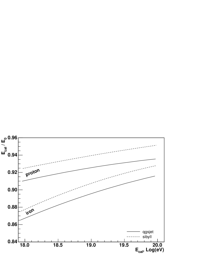
Figure 4: Missing energy correction plotted as the fraction $E_{cal}/E_{0}$ as a function of $E_{cal}$. The variation with the high energy hadronic interaction model is shown. Simulations for proton and iron primaries, at $45^{o}$.

The dependence on the interaction model is considerable, as shown in figure 4. We compared, for proton and iron at $45^{o}$, the missing energy correction curves obtained with QGSJET01 and SIBYLL2.1 models. The difference is practically constant: around $1.6\%$ for proton and $1.2\%$ for iron. In all cases, SIBYLL predicts less missing energy than QGSJET.

5 Conclusions

The energy deposit by atmospheric air showers was studied aiming for a better reconstruction of the primary energy. The new and very detailed energy balance now present in CORSIKA was used.

Our results for the missing energy correction function agree with previous calculations [14, 16], to within $1\%$. The dependence of this function on angle and observation level was found to be less than $0.7\%$. Comparing the high energy hadronic interaction models QGSJET and SIBYLL, the results differ by less than $1.6\%$. The larger dependence comes from the primary mass, being less than $5\%$ at $10^{18}eV$, decreasing with energy.

We found a mean parameterization of $E_{cal}/E_{0}$, taken as a mixture of $50\%$ proton and $50\%$ iron at $45^{o}$, as usually used in the reconstruction routines. Considering the QGSJET model only, we estimate that the total systematic error, introduced by the use of just this parameterization, is below $3\%$ at $1EeV$, and below $2\%$ at $100EeV$. This is of the order of shower-to-shower fluctuations. For proton showers, the rms value of $E_{cal}$ is $1.1\%$ of the primary energy. For iron showers, it is $0.4\%$.

particle	$E_{kin}\ (MeV)$	Rel. Contri. (%)	Ion. Frac. (%)
$\gamma$	.458	21.0	99.7 $\pm$ 0.4
$e^{+}$	4.29	20.9	99.7 $\pm$ 0.3	$f_{em}=99.8$
$e^{-}$	1.87	58.1	99.8 $\pm$ 0.5
$\mu^{+}$	8.30	48.7	43. $\pm$ 14.
$\mu^{-}$	8.26	51.3	42. $\pm$ 14.	$f_{\mu}=42.5$
$n$	43.2	22.9	57. $\pm$ 38.
$p$	35.6	18.0	98. $\pm$ 9.
$\pi^{0}$	86.0	27.5	99.7 $\pm$ 0.1
$\pi^{-}$	88.6	14.6	45. $\pm$ 16.
$\pi^{+}$	95.6	13.7	47. $\pm$ 16.	$f_{h}=73.9$
${}^{2}H$	37.2	1.7	99. $\pm$ 5.
${}^{3}H$	43.2	0.8	99. $\pm$ 6.
${}^{4}H$	41.4	0.3	99. $\pm$ 3.

Table 1: Particles discarded in air. Mean kinetic energy, relative contribution and fraction of energy going to ionization are shown. The fractions $f_{em}$, $f_{\mu}$ and $f_{h}$ are the average over all particles weighted by their relative contributions.

particle	$E_{kin}\ (GeV)$	Rel. Contri. (%)	Ion. Frac(%)
$n$	10.	7.12	70.1 $\pm$ 0.1
$p$	31.6	5.57	75.3 $\pm$ 0.1
$\bar{p}$	100.	3.21	73.2 $\pm$ 0.1
$\bar{n}$	100.	2.92	72.2 $\pm$ 0.1
$K^{0}_{L}$	1000.	7.30	36.3 $\pm$ 0.2	$f^{\prime}_{h}=61.0$
$K^{\pm}$	1000.	8.86	60.4 $\pm$ 0.2
$\pi^{-}$	316.	32.06	61.7 $\pm$ 0.2
$\pi^{+}$	316.	33.01	59.3 $\pm$ 0.2

Table 2: Hadrons at ground level. Mean kinetic energy, relative contribution and fraction of energy going to ionization are shown. The fraction $f^{\prime}_{h}$ is the average over all particles weighted by their relative contributions.

			gammas	electrons	muons	hadrons	neutrinos
		ION	- / -	64.7 / 65.3	1.0 / 1.5	0.2 / 0.3	- / -
	1EeV	CUT	1.1 / 1.2	10.7 / 10.8	0.1 / 0.1	0.3 / 0.5	3.0 / 4.6
		GRD	8.4 / 4.6	4.2 / 2.1	5.2 / 8.0	1.1 / 1.1	- / -
		ION	- / -	62.0 / 64.9	0.8 / 1.2	0.2 / 0.3	- / -
$0^{o}$	10EeV	CUT	1.1 / 1.2	10.2 / 10.7	0.1 / 0.1	0.3 / 0.4	2.5 / 3.6
		GRD	11.3 / 7.0	5.9 / 3.4	4.4 / 6.2	1.1 / 1.2	- / -
		ION	- / -	57.7 / 62.8	0.7 / 1.0	0.2 / 0.2	- / -
	100EeV	CUT	1.0 / 1.1	9.4 / 10.3	0.1 / 0.1	0.3 / 0.3	2.1 / 2.8
		GRD	15.2 / 10.1	8.4 / 5.1	3.7 / 4.9	1.2 / 1.3	- / -
		ION	- / -	69.8 / 67.6	1.2 / 1.8	0.2 / 0.3	- / -
	1EeV	CUT	1.3 / 1.3	13.0 / 12.7	0.1 / 0.1	0.4 / 0.5	3.3 / 5.0
		GRD	3.4 / 1.7	1.5 / 0.7	5.3 / 8.0	0.5 / 0.4	- / -
		ION	- / -	69.0 / 69.1	1.0 / 1.4	0.2 / 0.3	- / -
$30^{o}$	10EeV	CUT	1.3 / 1.3	12.9 / 12.9	0.1 / 0.1	0.4 / 0.4	2.7 / 3.9
		GRD	5.0 / 2.7	2.4 / 1.2	4.4 / 6.2	0.5 / 0.5	- / -
		ION	- / -	67.6 / 69.5	0.8 / 1.1	0.2 / 0.2	- / -
	100EeV	CUT	1.3 / 1.3	12.6 / 13.0	0.1 / 0.1	0.3 / 0.4	2.3 / 3.1
		GRD	7.0 / 4.0	3.6 / 1.8	3.7 / 5.0	0.5 / 0.5	- / -
		ION	- / -	71.2 / 67.2	1.4 / 2.0	0.2 / 0.3	- / -
	1EeV	CUT	1.5 / 1.4	15.6 / 14.7	0.1 / 0.1	0.4 / 0.5	3.6 / 5.4
		GRD	0.5 / 0.3	0.2 / 0.1	5.2 / 7.9	0.1 / 0.1	- / -
		ION	- / -	72.3 / 69.8	1.2 / 1.6	0.2 / 0.2	- / -
$45^{0}$	10EeV	CUT	1.5 / 1.5	15.8 / 15.3	0.1 / 0.1	0.4 / 0.5	3.0 / 4.2
		GRD	0.8 / 0.4	0.3 / 0.2	4.3 / 6.1	0.1 / 0.1	- / -
		ION	- / -	72.7 / 71.5	1.0 / 1.3	0.2 / 0.2	- / -
	100EeV	CUT	1.5 / 1.5	15.9 / 15.7	0.1 / 0.1	0.4 / 0.4	2.6 / 3.4
		GRD	1.2 / 0.7	0.5 / 0.3	3.7 / 4.8	0.1 / 0.1	- / -
		ION	- / -	67.5 / 63.4	1.7 / 2.3	0.2 / 0.2	- / -
	1EeV	CUT	1.7 / 1.6	19.2 / 18.1	0.1 / 0.1	0.5 / 0.6	4.1 / 6.1
		GRD	0.0 / 0.0	0.0 / 0.0	5.1 / 7.6	0.0 / 0.0	- / -
		ION	- / -	69.3 / 66.2	1.4 / 1.9	0.1 / 0.2	- / -
$60^{0}$	10EeV	CUT	1.7 / 1.7	19.7 / 18.8	0.1 / 0.1	0.4 / 0.5	3.3 / 4.7
		GRD	0.0 / 0.0	0.0 / 0.0	4.0 / 5.8	0.0 / 0.0	- / -
		ION	- / -	70.1 / 68.2	1.2 / 1.6	0.1 / 0.2	- / -
	100EeV	CUT	1.8 / 1.7	19.9 / 19.4	0.1 / 0.1	0.4 / 0.5	2.9 / 3.8
		GRD	0.0 / 0.0	0.0 / 0.0	3.5 / 4.6	0.0 / 0.0	- / -

Table 3: Mean energy deposit contributions (in percentage of primary’s energy) from different shower components. Each three lines correspond to a fixed choice of angle and energy, and discriminate: (ION) ionization in air, (CUT) simulation cuts and (GRD) particles arriving at ground. The first value (first/second) refers to proton showers while the second refers to iron showers.

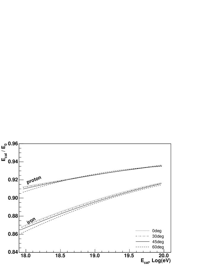
Figure 1: Missing energy correction plotted as the fraction $E_{cal}/E_{0}$ as a function of $E_{cal}$. The curves are for proton and iron showers at four different angles.

Coefficients of correction function
	Iron			Iron/Proton			Proton
angle	A	B	C	A	B	C	A	B	C
0	0.970	0.100	0.139	0.977	0.085	0.117	0.984	0.071	0.089
30	0.971	0.102	0.137	0.979	0.088	0.114	0.986	0.074	0.088
45	0.977	0.109	0.130	0.967	0.078	0.140	0.958	0.048	0.162
60	0.962	0.098	0.161	0.948	0.062	0.220	0.942	0.035	0.337

Table 4: Fitting parameters for different simulation conditions, as plotted in figure 1. The mid column indicates the $50\%/50\%$ mixture and the values corresponding to $45^{o}$ are bold faced. The fit function used was: $A-B(E/EeV)^{-C}$.

Figure 2: Missing energy correction plotted as the fraction $E_{cal}/E_{0}$ as a function of $E_{cal}$. The average between iron and proton missing energy correction is plotted. For comparison, Song’s and Linsley’s results are also shown.

Figure 3: Missing energy correction plotted as the fraction $E_{cal}/E_{0}$ as a function of $E_{cal}$. The dependence of the parameterization on ground level on ground level is shown. Simulations for proton and iron primaries, at $45^{o}$.

References

- [1] A. V. Olinto, Phys. Rep. 333-334 (2000) 329.
- [2] T. K. Gaisser, Nucl. Phys. B (Proc. Suppl.) 117 (2003) 318.
- [3] J. Cronin for the Auger Collaboration, Technical Design Report, The Pierre Auger Observatory, www.auger.org (1996).
- [4] T. Yamamoto for the Telescope Array Collaboration, Nucl. Instr. Meth. A 488 (2002) 191.
- [5] M. Teshima for the EUSO Collaboration, in: Proc. 28th ICRC, Tsukuba, 2003, p. 1069.
- [6] P. Dierickx, et al., in: Proc. Bäckaskog Workshop on Extremely Large Telescopes, 2000, p. 43.
- [7] R. M. Baltrusaitis, et al., Nucl. Instr. Meth. A 240 (1985) 410.
- [8] F. Kakimoto, et al., Nucl. Instr. Meth. A 372 (1996) 527.
- [9] M. Nagano, K. Kobayakawa, N. Sakaki, K. Ando, Astropart. Phys. 20 (2003) 293.
- [10] F. Arciprete, et al., in: Proc. 28th ICRC, Tsukuba, 2003, p. 837.
- [11] P. Hüntemeyer for the FLASH Collaboration, in: Proc. 28th ICRC, Tsukuba, 2003, p. 845.
- [12] E. Kemp, H. Nogima, L. G. dos Santos, C. O. Escobar, A. C. Fauth, in: Proc. 28th ICRC, Tsukuba, 2003, p. 853.
- [13] J. Linsley, in: Proc. 18th ICRC, Vol. 12, Bangalore, 1983, p. 135.
- [14] J. Linsley, in: Proc. 19th ICRC, Vol. 2, La Jolla, 1985, p. 154.
- [15] R. M. Baltrusaitis, et al., in: Proc. 19th ICRC, Vol. 7, La Jolla, 1985, p. 159.
- [16] C. Song, Z. Cao, B. R. Dawson, B. E. Fick, P. Sokolsky, X. Zhang, Astropart. Phys. 14 (2000) 7.
- [17] M. Risse, D. Heck, Astropart. Phys. 20 (2004) 661.
- [18] D. Heck, J. Knapp, J. Capdevielle, G. Schatz, T. Thouw, Tech. Rep. FZKA 6019, Forschungszentrum Karlsruhe, www-ik.fzk.de/heck/corsika (1998).
- [19] N. N. Kalmykov, S. S. Ostapchenko, A. I. Pavlov, Nucl. Phys. B (Proc. Suppl.) 52B (1997) 17.
- [20] D. Heck, et al., in: Proc. 27th ICRC, Vol. 1, Hamburg, 2001, p. 233.
- [21] H. Fesefeldt, Tech. Rep. PITHA-85/02, RWTH Aachen (1985).
- [22] M. Kobal for the Pierre Auger Collaboration, Astropart. Phys. 15 (2001) 259.
- [23] M. Risse, D. Heck, J. Knapp, S. Ostapchenko, in: Proc. 27th ICRC, Vol. 2, Hamburg, 2001, p. 522.
- [24] A. M. Hillas, Nucl. Phys. B (Proc. Suppl.) 52B (1997) 29.
- [25] R. Engel, T. Gaisser, P. Lipari, T. Stanev, in: Proc. 26th ICRC, Vol. 1, Salt Lake City, 1999, p. 415.
- [26] R. S. Fletcher, T. Gaisser, P. Lipari, T. Stanev, Phys. Rev. D 50 (1994) 5710.
- [27] R. Engel, T. Gaisser, P. Lipari, T. Stanev, Phys. Rev. D 46 (1992) 5013.
- [28] S. Agostinelli, et al., Nucl. Instr. Meth. A 506 (2003) 250.