The Evolution of Early-type Field Galaxies Selected from a NICMOS Map of the Hubble Deep Field North

Abstract

The redshift distribution of well-defined samples of distant early-type galaxies offers a means to test the predictions of monolithic and hierarchical galaxy formation scenarios. NICMOS maps of the entire Hubble Deep Field North in the F110W and F160W filters, when combined with the available WFPC2 data, allow us to calculate photometric redshifts and determine the morphological appearance of galaxies at rest-frame optical wavelengths out to $z\sim 2.5$. Here we report results for two subsamples of early-type galaxies, defined primarily by their morphologies in the F160W band, which were selected from the NICMOS data down to ${H_{160}}_{AB}<24.0$. A primary subsample is defined as the 34 galaxies with early-type galaxy morphologies and early-type galaxy spectral energy distributions. The secondary subsample is defined as those 42 objects which have early-type galaxy morphologies with non-early type galaxy spectral energy distributions. The observed redshift distributions of our two early-type samples do not match that predicted by a monolithic collapse model, which shows an overabundance at $z>1.5$. A $\langle V/V_{max}\rangle$ test confirms this result. When the effects of passive luminosity evolution are included in the calculation, the mean value of $V_{max}$ for the primary sample is $0.22\pm 0.05$, and $0.31\pm 0.04$ for all the early-types. A hierarchical formation model better matches the redshift distribution of the HDF-N early-types at $z>1.5$, but still does not adequately describe the observed early-types. The hierarchical model predicts significantly bluer colors on average than the observed early-type colors, and underpredicts the observed number of early-types at $z\sim 2$.

Though the observed redshift distribution of the early-type galaxies in our HDF-NICMOS sample is better matched by a hierarchical galaxy formation model, the reliability of this conclusion is tempered by the restricted sampling area and relatively small number of early-type galaxies selected by our methods. For example, our results may be biased by the way the HDF-N appears to intersect a large scale structure at $z\sim 1$. The results of our study underscore the need for high resolution imaging surveys that cover greater area to similar depth with similar quality photometry and wavelength coverage.

Though similar in appearance in the ${H_{160}}$ data, the primary and secondary samples are otherwise rather different. The primary sample is redder, more luminous, larger, and apparently more massive than the secondary sample. Furthermore the secondary sample shows morphologies in the optical WFPC2 images that are more often similar to late-type galaxies than is the case for the primary sample. The bluer secondary sample of early-types have a star formation history which can be approximated by a Bruzual & Charlot $\tau$ model, or by a galaxy formed at high redshift with a small, recent starburst. Given the differences in their apparent stellar masses and current luminosities, it would seem unlikely that the secondary sample could evolve into galaxies of the primary sample.

1 Introduction

An understanding of the evolution of elliptical galaxies continues to elude both observational astronomers and theoretical astrophysicists. The debate between two competing theories for the formation and evolution of elliptical galaxies has been guiding most recent investigations in this area. The traditional monolithic collapse model proposed by, e.g., Eggen, Lynden-Bell, & Sandage (1962), Searle, Sargent, & Bagnuolo (1973), and Tinsely & Gunn (1976) postulates a single burst of star formation at high redshift, followed by passive stellar evolution. The newer alternative is based in a cold dark matter cosmogony, wherein galaxies are assembled hierarchically over relatively long periods of cosmic time. A detailed review of the observational evidence for and against both the monolithic and the hierarchical scenarios has been presented by Schade et al. (1999).

Significant observational effort has been spent in investigating these two galaxy formation scenarios. Attempts to uniformly select and study samples of high redshift early-types in the field have used selection criteria based on morphology, color, or both. There is little evolution in the luminosity function of red galaxies at $z<0.7$ in the CFRS (Lilly et al., 1995), which appears to contradict basic expectations of passive luminosity evolution (PLE) models, wherein galaxies should be more luminous at higher redshift. Reasonable interpretations are that ellipticals assemble late by merging processes, or that some fraction of distant ellipticals are blue enough to drop out of color-selected samples. Indeed, morphologically defined samples have identified blue field ellipticals (Schade et al., 1999; Menanteau et al., 1999; Treu et al., 2002; Im et al., 2002). Another possible interpretation of the CFRS results is that galaxies grow in mass through merging while simultaneously fading. The issue of the mass of these blue early-types was addressed by Im et al. (2001) who suggest that most of the blue spheroidals being found in the field at moderate redshifts are low-mass systems undergoing starbursts, rather than massive ellipticals.

Several studies using morphological identification of early-types in optical HST images have found little if any change in the space density of ellipticals up to $z\sim 1$ (Driver et al., 1998; Brinchmann et al., 1998; Im et al., 1999; Schade et al., 1999). At $z>1$, the strong k-correction means that near-IR data are better suited to making an unbiased census of early-types. In the two Hubble Deep Fields (HDF), studies using ground-based near-IR imaging have found a deficit of red ellipticals at $z>1$ (Zepf, 1997; Franceschini et al., 1998; Barger et al., 1999). More extensive optical-IR surveys incorporating morphologies based on data from WFPC2 (Im et al., 1999; Menanteau et al., 1999; Abraham et al., 1999) or NICMOS (Treu & Stiavelli, 1999) have also concluded that there are fewer luminous, red ellipticals at $z>1$ than would be expected from PLE models. IR surveys of larger areas which rely on colors instead of morphologies to select early-types have found a variety of values for the space density of red galaxies at higher redshifts (McCracken et al., 2000; Daddi et al., 2000; McCarthy et al., 2001).

A continuing source of uncertainty in the interpretation of such surveys is the way that large scale structure may influence the results given the relatively small areas typically covered in near-IR imaging surveys. Our study is particularly affected by this problem because red galaxies cluster even more strongly than do field galaxies in general. Daddi et al. (2001) found a comoving correlation length $r_{0}h=12\pm 3$ Mpc for a sample of 400 extremely red galaxies ($R-K_{s}>5$ to $K_{s}=19.2$) in a 700 arcmin² survey. Another problem when comparing deep fields such as the HDF to a local galaxy population in order to measure evolution is the uncertainty in the faint end of the local galaxy luminosity function. Since the HDF data reach such faint magnitudes, the majority of the galaxies have low luminosities, and hence the comparison with the local population is sensitive to the faint end slope. Improvements in our knowledge of the local LF due to the Two Degree Field Survey and the Sloan Digital Sky Survey should help to alleviate this problem in the near future.

Due to the extreme depth of its high resolution imaging, the HDF comes into its own in the important redshift regime of $1<z<2$. The large observed wavelength range and accuracy of the combined WFPC2 and NICMOS data makes it possible to obtain relatively accurate photometric redshifts for those objects without spectroscopic redshifts. By making use of our NICMOS map of the entire HDF in the $J_{110}$ and $H_{160}$ bands, we can exploit a dataset which is unique in being able to study the rest frame optical properties of high redshift early-type galaxies. The available dataset allows us to largely solve problems having to do with the adequate and consistent selection of early-type galaxies up to redshifts high enough ($z\sim 3$) to reach their likely formation epoch(s). Recently, Dickinson, Papovich, & Ferguson (2003) have exploited the advantages of the same dataset to examine the evolution of the global stellar mass density at $z<3$.

Though dependent on the details and on the particular cosmology, in general terms the two galaxy formation scenarios predict significantly different histories for the evolution of the space density of early-type galaxies. Assuming a single formation epoch, the number of E-S0s in a given mass range remains constant with time in the monolithic model. In a hierarchical model, the situation is more complex. Early type galaxies can grow in mass by merging, or acquire a new disk and become ’late type’. As a general trend, the number of massive early type galaxies should increase with time in this scenario. The space density test is potentially the most powerful in distinguishing between the two formation scenarios. There are at least two significant problems relevant to our investigation in carrying out such an experiment. First, we typically measure brightness and redshift to calculate the luminosity of a galaxy, but do not know the mass. Currently the best practical method of overcoming this problem for a large, faint sample is to determine the luminosity of a galaxy as close in wavelength as possible to the rest frame near-IR, where the mass-luminosity relation is most stable against perturbations from dust and recent star formation. In the future it may become feasible to obtain a more accurate dynamical measure of the mass for large numbers of distant galaxies. Second, we must select early-type galaxies from observational surveys. This second problem can be addressed by obtaining the highest resolution images possible and performing a morphological selection.

Though such a morphological method of selecting early-types may be the best available, it is not without potential pitfalls. Even with the excellent HST angular resolution and deep images of the HDF, morphological classification of very faint galaxies is difficult. Selection biases as a function of magnitude, redshift, and galaxy type are probable. We describe below tests using simulations in an attempt to both quantify these biases and to qualitatively understand them.

Another potential problem with the morphological selection technique could occur if an early-type galaxy were undergoing an interaction or were forming during a major merger event. Then it might not be classified as an “early type” and thus could be excluded from our sample. Similarly, the recent advances made by SCUBA in finding evidence of dust-enshrouded star formation at high redshift also has complicated understanding of the origin of early-type galaxies. It may be that the high-$z$ SCUBA sources will become early-type galaxies, but that these sources are too heavily obscured to show up in deep near-IR imaging surveys. If the antecendents of today’s early–type galaxies cannot be recognized by their morphologies at high redshift, then it will be difficult to wisely choose adequate samples for comparison with present–epoch ellipticals.

This paper presents the results of our investigation of early-type galaxy evolution, based on deep NICMOS and WFPC2 images of the HDF–N. We will describe the way early-type samples may be selected by using morphology and/or on the basis of the colors. These samples are then compared with the predictions of monolithic collapse and of hierarchical models. Though the results of these comparisons are clear, their significance to understanding elliptical and S0 galaxy formation and evolution is tempered by the fact that the HDF-N represents only one very small window into the Universe, which may be strongly affected by large scale structure. Perhaps more valuable are the results obtained from comparing the subsamples of red and blue early-types concerning the nature of early-type galaxy evolution. The assumed cosmological parameters are $h=H_{0}/(100$ km s^-1 Mpc${}^{-1})=0.7$, $\Omega_{M}=0.3$, and $\Omega_{\Lambda}=0.7$. Over the redshift range of interest, the linear resolution of the data does not change by much. Approximately 90% of the early-types found in the NICMOS data span a redshift range such the linear resolution varies by a factor of only 1.43.

2 Data

The HDF–N was observed by NICMOS between UT 1998 June 13 and June 23, when the HST secondary mirror was at the optimal focus for Camera 3. Our observations and data reduction will be described in detail elsewhere (Dickinson et al. in preparation); the relevant aspects are summarized here. The complete HDF–N was mosaiced by Camera 3 with 8 sub–fields, each imaged during three separate visits. During each visit, exposures were taken through both the F110W (1.1$\mu$m) and F160W (1.6$\mu$m) filters. (Henceforth we will refer to the six WFPC2 and NICMOS HDF bandpasses used on the HDF-N as $U_{300}$, $B_{450}$, $V_{606}$, $I_{814}$, $J_{110}$ and $H_{160}$.) Each section of the mosaic was dithered through 9 independent positions, with a net exposure time of 12600s per filter, except in a few cases where telescope tracking was lost due to HST Fine Guidance Sensor failures.

The data were processed using STScI pipeline routines and custom software, and were combined into a single mosaic, accurately registered to the HDF–N WFPC2 images, using the “drizzling” method of Fruchter & Hook (2002). The Camera 3 images have a point spread function (PSF) with FWHM $\approx$ 0$\hbox to0.0pt{.\hss}{{}^{\prime\prime}}$22, primarily limited by the pixel scale (0$\hbox to0.0pt{.\hss}{{}^{\prime\prime}}$2). Sensitivity varies over the field of view due to variations in NICMOS quantum efficiency and exposure time. On average the images have a signal–to–noise ratio $S/N\approx 10$ within a $0\hbox to0.0pt{.\hss}{{}^{\prime\prime}}7$ diameter aperture at $AB\approx 26.1$ for both the $J_{110}$ and $H_{160}$ filters. In order to ensure properly matched photometry between the optical and infrared images, the WFPC2 data were convolved to match the NICMOS PSF. Photometric catalogs were constructed using SExtractor (Bertin & Arnouts, 1996), by detecting objects in a sum of the $J_{110}$ and $H_{160}$ images and then measuring fluxes through matched apertures in all bands. Objects were classified as star, and removed from the catalog, as a result of spectroscopic information, of having colors similar to stars, of their point-like appearance in the HST images, and of their having high CLASS_STAR values according to SExtractor. The complete galaxy catalog down to $H_{160}$ $<26.0$ will be referred to as the HDF NICMOS Mosaic, or HNM, catalog. Information for the ${H_{160}}<24.0$ sample is presented in Table 1, including catalog number, the ”total” i.e. MAG_AUTO magnitude $H_{160}^{k}$, and the isophotal ${I_{814}}-{H_{160}}$ color, as well as other parameters to be defined in later sections. MAG_AUTO is the magnitude measured within an ellipse whose size is defined by radial moments of the light profile (Kron, 1980), and is designed to enclose a large and roughly constant fraction of the galaxy light for a variety of surface brightness profiles.

Additional $K$-band photometry was obtained from the imaging carried out by Dickinson (1998) on the HDF-N using IRIM on the KPNO 4 m telescope. A version of the fitting procedure described by Fernandez-Soto, Lanzetta, & Yahil (1999) was implemented by Papovich, Dickinson, & Ferguson (2001) to optimally measure photometry from the ground-based images which had been matched to the HST images.

3 Sample Definition

To produce samples of early-type galaxies, we have followed three methods to select objects from the HNM catalog at $H_{160}$ $<24.0$: classical Hubble typing by visual inspection, de Vaucouleur function fitting of surface brightness profiles, and the construction of galaxy spectral types that result from photometric redshift estimates. The three early-type selection methods express traditional ideas about the definition of early-type galaxies, and are described below in more detail.

3.1 Visual Classification

As a first attempt to obtain basic morphological information on the objects in the HNM catalog, the $H_{160}$ images of all 230 objects with ${H_{160}}<24.0$ were visually inspected by 7 members of the NICMOS GO program team. Hubble types were assigned by each classifier for each object where possible. The typing became difficult for the smallest objects; some classifiers did not assign types in these cases. The Hubble types were converted to T-types (hereinafter TT). The T-types for common Hubble types are as follows: $E=-5,S0=-2,Sa=1,Sb=3,Sc=6$, and $Im=10$ (RC3). Objects which were found to be too compact for classification were given a TT of $-$10. The T-types were averaged and the rms calculated. Objects for which the rms of the TT was relatively large (greater than $\sim$3) were reconsidered. In most of these cases, the T-type assigned by one classifier was significantly different from the other values. In these cases, the discrepant value was discarded, the T-type recalculated and compared with the visual appearance in all of the available HST bands. In some of these cases, the assigned T-types were distributed over a large range, accounting for the large rms on the average. These T-types could not be reconciled and so the original average value is retained along with its large rms, signifying a very uncertain classification. The average T-types are plotted against their $H_{160}$ magnitudes in Figure 1, and are listed in Table 1 along with their uncertainties. Images of all of the objects in this catalog may be viewed by accessing the website www.stsci.edu/$\sim$med/hdfnic3.

Another visual classification was also performed by one of the authors (SAS). The $HST$ band which most closely samples the rest frame $B$-band, called $B_{r}$, for each object was used to determine its T-type. The redshifts used for this procedure were spectroscopic where available; otherwise photometric redshifts (see Section 3.3) were used. The highest redshift that could be typed in this manner was $z\sim 3$. Beyond this redshift, the necessary observed band has a wavelength redder than the available $HST$ imaging. In general, the $B_{r}$ T-types agree with the average values determined from the observed $H_{160}$ image. In Figure 2, the difference in T-types determined from the $H_{160}$ and $B_{r}$ images is shown as a function of $H_{160}$ T-type. Little systematic trend is evident. Similarly, in Figure 3, the redshift distribution of the TT differences does not show a systematic trend with redshift. The TT determined from the ${H_{160}}$ band is used for all morphological types in the rest of this work.

To determine the biases in the visual classifications, we performed the following test. The $B$ and $g$ images from the Frei et al. (1996) sample of nearby galaxies were transformed so as to appear to be $L^{\ast}$ galaxies at $z=0.75$ with the S/N of our data and then convolved with the NIC3 F160W PSF. These images were then visually classified by four of the authors and a comparison made with the known T-types from the RC3. This test found a tendency to classify galaxies towards earlier types by $\sim$0.7 T-types on average, with the rms on the average difference between the classified and real T-type being $\sim$2.8. Because of surface brightness dimming, it would be natural to suspect that we would preferentially assign earlier types to higher redshift objects if the fainter disks are harder to see with increasing $z$. While our test suggests that this has not happened with our classifications of the NIC3 images, it is not possible to rule out the surface brightness dimming bias completely. The distribution of assigned T-type against redshift is shown in Figure 4, where we see that higher redshift objects have a slight tendency to have been given later T-types. However we do not know the intrinsic distribution of T-types as a function of redshift. Indeed even though the HST resolution is high, the amount of resolved detail in physical terms in the highest redshift objects is still less than for the lower redshift objects. So it would be likely for the assigned morphologies of the highest redshift objects to be biased. Probably even more important in the context of these tests is that the lower spatial resolution of the NIC3 camera significantly reduces the apparent contrast of structural features such as spiral arms.

The distribution of Hubble types, based on the assigned T-types, is shown for the ${H_{160}}<24.0$ sample in a color magnitude diagram in Figure 5. If early-type galaxies are defined as those objects with $-7\lesssim$T-type$\lesssim-2$, then there are 66 such galaxies in the HNM catalog down to $H_{160}$ $=24.0$.

3.2 Profile Fitting

Another method was employed to define early-type galaxies in the HNM sample by using profile fitting. Elliptical isophotes were fit to the $H_{160}$ images of each object. The center of each ellipse was held fixed while the position angle and ellipticity were allowed to vary with semimajor axis during the fitting. The resulting surface brightness profile was fit by a convolution of a de Vaucouleur’s law with the NIC3 F160W PSF. The fitting was done over a range in radius of $0\farcs 08<r<2\farcs 0$ and the model with the lowest $\chi^{2}$ was chosen as being the best fit. Simulations were performed of this procedure, using model galaxies with de Vaucouleur profiles and known $r_{e}$, to determine how well $r_{e}$ could be determined. These models included the effects of the background level and the PSF. As shown in Figure 6, over the range $0\farcs 3<r_{e}<1\farcs 1$ and $24<{H_{160}}<20$, $r_{e}$ is found to vary within 25% of the input value using our fitting parameters.

The best fit $r_{e}$, $\mu_{e}$ (the half-light radius and the average surface brightness within that radius) were recorded along with a visual estimate of the quality of the fit for each galaxy in the ${H_{160}}<24.0$ sample. These quality estimates are given in the column labelled “q” in Table 1, with p representing poor, f for fair, and g for good. These qualitative classifications were deemed adequate because the profile fitting is not being used as the main method of selecting the early-type galaxies. In cases where the object is obviously e.g. an irregular galaxy, the fits are essentially meaningless; these are classified as poor fits. For some objects, the quality of the fit to the surface brightness profile by the $r^{1/4}$ law is fair but not good enough to exclude a reasonable fit by an exponential profile. The objects where the fit to the surface brightness profile is good may be considered to be early-type galaxies; there are 52 such objects in the HNM down to ${H_{160}}<24.0$. Examples of the profile fits are shown in Figure 7.

3.3 Photometric Redshifts and Spectroscopic Types

Spectroscopic redshifts are used where available and are listed in Table 1. These have been taken from the literature, mostly taken from Cohen et al. (2000); Cohen (2001), and Dawson et al. (2001) and references therein, along with a few redshifts made available by C. Steidel and K. Adelberger (private communication). For those objects without spectroscopic redshifts, photometric redshift estimates were obtained from Budavári et al. (2000) who used all 7 bands for which we have photometry; the 6 HST bands plus the $K$-band data from KPNO. A comparison between the best-fit photometric $z$ and the spectroscopic redshifts, where available, may be seen in Figure 8. As described fully in Budavári et al. (2000), the best fitting combination of 3 eigenspectra from Coleman, Wu, & Weedman (1980) at the most likely redshift is used to obtain the galaxy spectral type (hereinafter the S-type or ST), for each object, which is listed in Table 1, along with the photometric redshift. For our purposes we have chosen to define early-type galaxies as having spectral types less than 0.2. We decided to use a higher value of 0.2, compared to the value of 0.1 given by Budavári et al. (2000), to define an early-type SED because a higher value allows for some evolution in the SED towards bluer colors at higher redshifts which has been found to occur in early-type galaxies (sed98). An early-type ST is a galaxy whose SED is dominated by an old stellar population, which is not necessarily the same thing as a galaxy with an early-type morphology. We will make use of these two definitions of what constitutes an early-type galaxy below in selecting different kinds of early-type samples from the HNM. For reference Sa, Sc, and Irr galaxies have ST values of 0.15, 0.35, and 0.55 respectively. If galaxy spectral type is the only criterion, 54 galaxies with S-type values less than 0.2 would be selected from the HNM sample down to ${H_{160}}=24.0$.

3.4 Primary and Secondary Subsamples

A useful way to compare the three ways of defining early-type galaxies is shown in Figure 9. The galaxy spectral types are plotted against the T-types, with the quality of the de Vaucouleur fit being indicated by the point style. A very broad correlation is seen from the combination of earlier T-type and earlier S-type to later T-type and later S-types. But there is a large amount of scatter in the other parameter at a given T-type or S-type. Nominally the S-type value should be less than 0.1 to qualify as an elliptical or S0 galaxy, according to the photometric redshift methodology, and the T-type should be less than $\sim$0. Figure 9 shows a well-defined group of galaxies with $-7<$ T-type $<-2$ but with S-types reaching as high as $<0.2$; note that all of these galaxies have fair to good $r^{1/4}$ law fits. This combined definition may be a good way to isolate true early-type galaxies, though it is not without caveats. The objects with S-types at $0.1-0.2$ may be better fit by the photo-z technique using later-type spectra because their dominant stellar populations are younger than a present-epoch elliptical—as would be expected at higher redshifts. Furthermore, some of the objects in this group have profiles which are fit by exponential profiles as well as by the de Vaucouleur law, indicating a significant contribution from a disk component to the observed $H_{160}$ light is possible. Finally, there are a significant number of galaxies outside of this group in Figure 9 which qualify as early-type galaxies in at least two of the three methods. Only selecting objects with S-types less than 0.1 would add few objects to the group of apparent early-types, principally with later T-types and a mixture of profile fit qualities. Selecting galaxies just by T-type would add a significant number of apparent early-types spanning a large range in spectral type, with mostly fair to good $r^{1/4}$ law fits. Selecting galaxies just by their profile fits would add mainly the same objects as the T-type selector. In short, the T-type and profile fitting methods agree the best amongst the various combinations; this is not surprising, given that they are morphological selectors, while the S-type has to do more with stellar evolution.

We choose to define the 34 galaxies in Figure 9 with $-7<$ T-type $<-2$ and $0<$ S-type $<0.2$, all of which have fair to good $r^{1/4}$ law fits, as the primary sample of early-types in the HNM catalog at ${H_{160}}<24.0$. 16 of these 34 galaxies have spectroscopic redshifts. Also, we define a secondary early-type sample as those 42 objects outside of the primary early-type area in Figure 9, which have $-7<$ T-type $<0$ and fair or good $r^{1/4}$ law fits. 21 of these 42 galaxies have spectroscopic redshifts. Montages of color images of all galaxies in both the primary and secondary samples are shown in Figure 10 and Figure 11, respectively. For each galaxy, two images are shown; one based on a combination of the $IJH$ bands and the other on the $BVI$ bands. For both the primary and secondary samples, the images made from the redder bands generally appear to be early-type galaxies. However, the bluer band images of the secondary sample sometimes show evidence of late-type galaxy morphology.

The F160W images of the galaxies in the primary and secondary samples were examined to look for the incidence of close neighbors. One can imagine that the bluer colors of the secondary early-types could be due to galaxy interactions. We found no difference in the frequency of close neighbors between the two samples. There is a greater frequency of poor $r^{1/4}$ fits among the galaxies in the secondary sample relative to the primary sample. A plot of the rest frame $B-V$ color against the asymmetry index $A$ (Conselice, 2003) in Figure 12 shows only a small difference in the distributions in $A$ of the two early-type samples, with the secondary sample having a slightly higher mean value of $A$.

The combined primary and secondary samples form a set of early-type galaxies selected by morphology. One of the main goals of this paper is to understand the relationship between these two kinds of early-type galaxies.

4 Detection Simulations

To determine if and how we are affected by biases in detecting early type galaxies at high redshifts, we perform two different types of simulations. In the first, we simulate how 16 nearby giant elliptical galaxies would appear at $z\sim 2$ if observed under the same conditions in which the NICMOS HDF images were taken. We use the B-band images of NGC 2768, NGC 2775, NGC 4125, NGC 4365, NGC 4374, NGC 4406, NGC 4429, NGC 4442, NGC 4472, NGC 4486, NGC 4526, NGC 4621, NGC 4636, NGC 4754, NGC 5322 and NGC 5813 from the Frei et al. (1996) sample to perform these simulations. These galaxies cover the absolute magnitude range $-23<M(B)<-19$. K-corrections were applied to the simulated galaxies, but no correction was made for evolution. The luminosity and physical size of each galaxy were preserved during the transformation to $z=2$. The galaxy images were convolved with the NIC3 PSF and placed into an image that mimics the actual F160W image of the HDF-N in terms of sky level and photon noise. SExtractor was then run on this image. We find that we easily detect all 16 of the simulated galaxies.

We perform a similar simulation in which we take all the galaxies in the Hubble Deep Field with M${}_{\rm B}<-18$ and $0.4<z<0.8$ and place them at higher redshifts as they would be observed under the conditions in which the NICMOS data was taken. To make the simulated galaxies, the NIC3 PSF was used. When these galaxies are placed at $z\sim 2$ into an artificial NICMOS F160W band image which mimics the real NIC3 image of the HDF-F in terms of the sky level and noise, and then re-detected with the same SExtractor detection criteria used on the original $H_{160}$ band images, we find 100% are retrieved. In fact, the detection completeness does not begin to drop until $z\sim 2.5$, a much higher redshift than that of the decline in the observed ellipticals. We therefore conclude that it is unlikely that we are missing elliptical galaxies at $z>1.5$ due to our inability to either detect or identify these systems if they were present.

5 Evolution of Early-type Galaxies

We will examine the evolution of the early-type samples described above in two ways. First, the spectral evolution of the primary and secondary samples will be compared and contrasted. Second, the space density as a function of redshift will be compared with the predictions of a monolithic formation model and of an hierarchical model.

5.1 Spectral Evolution

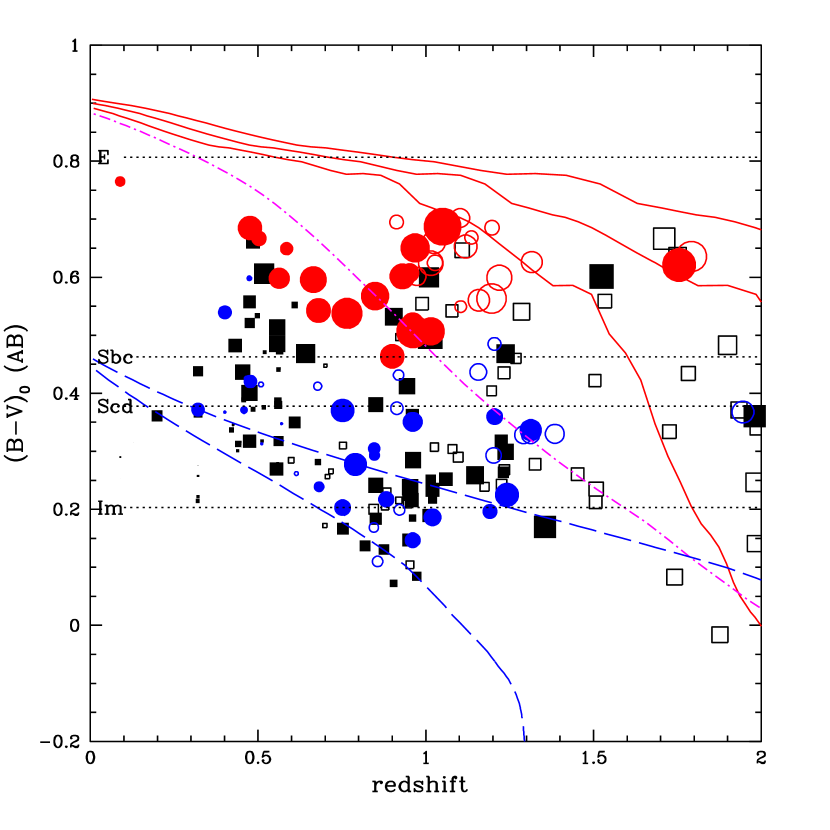
Figure 13: Rest frame $B-V$ colors against redshift. Red circles are primary early-types, and blue circles are secondary early-types. The squares are all other galaxies in the ${H_{160}}<24.0$ sample. Filled symbols have spectroscopic redshifts and open symbols have photometric redshifts only. The horizontal dashed lines are the colors of CWW spectral templates. The curves represent the colors of Bruzual & Charlot models described in the text. The solid red curves represent a 0.1 Gyr burst which starts at $z_{f}=5,3,2.1$ followed by passive luminosity evolution. The magenta dot-dash line is a $\tau=1$ Gyr exponential model with $z_{f}=2.5$, and the two blue, long-dash lines are $\tau=5$ Gyr exponential models with $z_{f}=1.5$ and $z_{f}=5$.

One of the traditional means of analyzing the evolution of galaxy populations is through the comparison of their colors with spectral synthesis models. We make one comparison in rest frame $B-V$ so as to consistently sample the same part of a galaxy’s rest frame spectrum. The rest frame colors for the objects were obtained by interpolating among the appropriate observed frame magnitudes as indicated by the redshift. Figure 13 shows the rest frame $B-V$ colors of all the $H<24$ sample with $M(V)<-17$, where the symbol size scales with $M(V)$. We have calculated the color evolution for a number of Bruzual & Charlot (1998 version) models with varying star formation histories, assuming only $Z_{\odot}$ stars and shown these in Figure 13. Most of the early-type galaxies lie between the single-burst $z_{f}=5$ and the $\tau$ models, indicating a wide range in star formation histories. Lower metallicity single burst models would yield bluer colors which could match the colors of the lower-redshift early-types that follow the $\tau$ model. Also, it would take only very small starbursts, in terms of the stellar mass, to make the high redshift $z_{f}$ PLE models blue enough to match the colors, if only for a short time, of the secondary early-types. Thus, the possibility that the early-types in the secondary sample formed the vast majority of their stars at high redshift cannot be excluded.

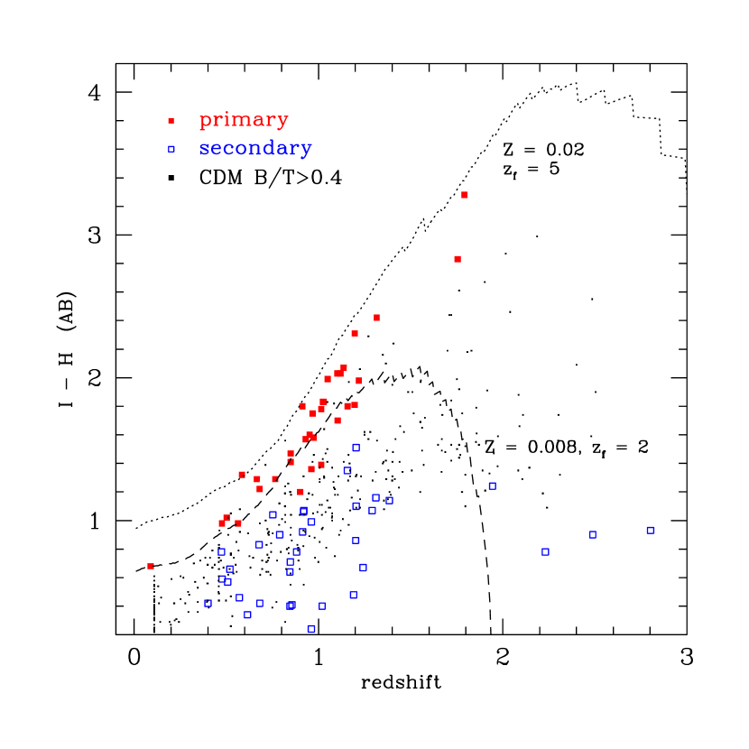
Figure 14: The $I-H$ color against redshift for the primary and secondary early-types in the HNM along with the simulated galaxies selected from the hierarchical model with a ratio of bulge/total light $>0.4$ in the ${H_{160}}$ band. Two Bruzual & Charlot PLE models are shown for reference.

It is also of interest to examine the spectral evolution of the hierarchical model (Somerville, Primack, & Faber (2001); see Section 5.3) galaxies relative to the early-types in the HDF-N by examining the observed colors vs redshift. We do so in Figure 14 which shows the $I-H$ color against redshift. Both the primary and secondary early-type samples are shown, along with model early-type galaxies selcted from the hierarchical simulations by their bulge to total ratio. For reference we have plotted the tracks corresponding to two extremes of the BC PLE models, one with a solar metallicity/high $z_{f}$ and the other with low metallicity/low $z_{f}$. As can be seen, the hierarchical model galaxies better follow the distribution of the secondary set of real early-type galaxies with the bluer colors at all redshifts, but do not reproduce the red envelope of the primary subsample. Also the model galaxies from the simulations are far more numerous at high redshifts compared to all the early-types that we selected from the HDF-N. Thus Figure 14 does not lend support to the hierarchical model being an adequate description of the early-type samples.

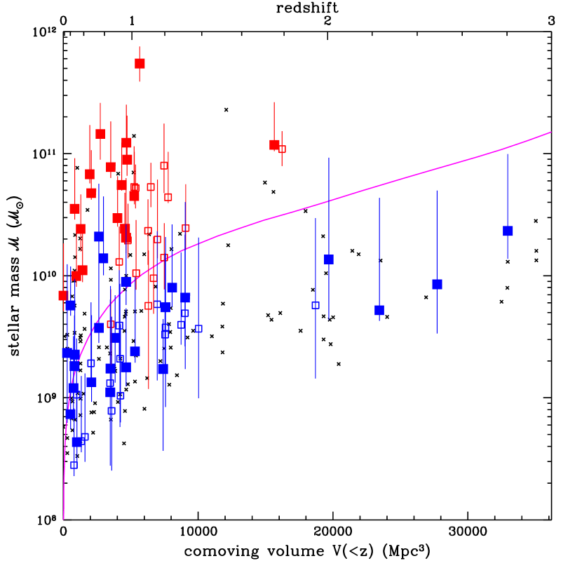
Figure 15: Estimated stellar mass against comoving volume and redshift for all galaxies in the HDF-N with ${H_{160}}<24.0$. The primary sample are plotted in red and the secondary sample are in blue. Open squares indicate photometric redshifts and solid squares are spectroscopic redshifts. The error bars show the 68% confidence range on mass, where the upper error bar comes from the one $\sigma$ upper limit from the 2-component models, and the lower error bar shows the one $\sigma$ lower limit from the 1-component model (see Papovich, Dickinson, & Ferguson 2001 for details). The small black crosses are the non early-type galaxies. The magenta line shows the mass limit corresponding to ${H_{160}}=24.0$ for a PLE star burst formed at $z=\infty$.

Papovich, Dickinson, & Ferguson (2001) and Dickinson, Papovich, & Ferguson (2003) report estimates for the stellar masses of galaxies selected from the same HDF NICMOS data. We make use of their 1-component fits which use monotonically-declining exponential star formation rates including dust, and show in Figure 15 the stellar masses for the galaxies with ${H_{160}}<24.0$ in the HDF-N. Clearly the primary early-type galaxies are more massive on average, at all redshifts, than the secondaries.

5.2 Scaling Relations

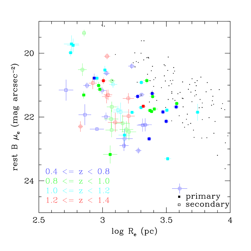
Figure 16: The rest frame $B$ $\mu_{e}$ against log of the $R_{e}$ for the two early-type samples. One $\sigma$ errorbars are shown on each point. Redshift information is encoded by the color of the points as indicated in the legend. The values of $R_{e}$ and $\mu_{e}$ have been corrected for the bias seen in Figure 6. The solid black dots represent ellipticals at $z\sim 0$ from Jorgensen, Franx, & Kjaergaard (1996).

Lacking velocity dispersions, we can use projections of the Fundamental plane to examine the differences between the primary and secondary samples of early-types. Figure 16 plots $\mu_{e}$ in the rest frame $B$ against the log of the $R_{e}$ which were measured by the $r^{1/4}$ fitting. It is interesting that in Figure 16 the secondary sample of bluer galaxies is more compact for a given surface brightness, consistent with these galaxies having an enhancement of light in their cores, possibly due to recent star formation (Menenteau et al., 2001). Figure 9 shows that there are very few galaxies with good de Vaucouleur profiles that are also blue and classified as morphological late types.

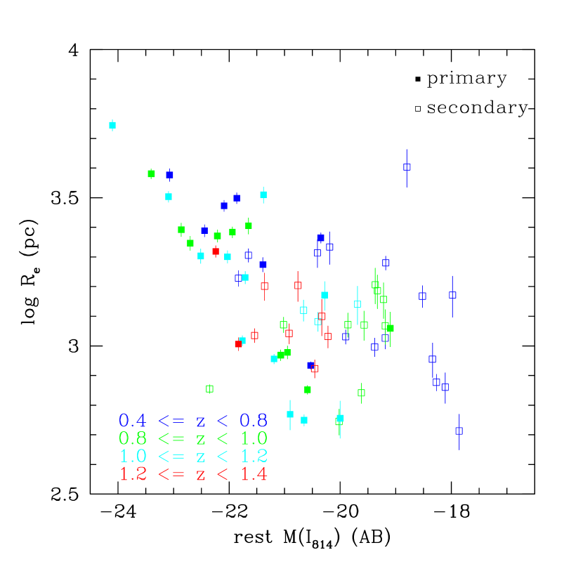
Figure 17: Log of the $R_{e}$ against $M({I_{814}})$ for the two early-type samples. One $\sigma$ errorbars are shown on each point based on simulations of the $r_{e}$ measurements. The point color encodes the redshift as indicated in the legend. The values of $R_{e}$ have been corrected for the bias in measuring $r_{e}$ found in our simulations and seen in Figure 6.

At $z<1$, Schade et al. (1999) have examined projections of the Fundamental Plane using WFPC2 images of field elliptical galaxies selected from the CFRS/LDSS. They found evolution with redshift in the relation between $R_{e}$ and $M(B)$ in the sense that the higher redshift galaxies are more luminous for a given size. The distributions in Figure 17 agree with this trend although the scatter is large in our measurements. It is clear that there are almost no large secondary early-types, whereas there are quite a few large primary early-types: there are 4 secondaries and 17 primaries with $R_{e}>2$ kpc.

5.3 Number Density

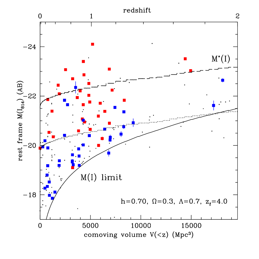
Figure 18: The rest frame $M(I_{814})$ against the comoving volume of the whole survey for the two early-type samples: the red, solid points are the primary sample and blue, open points are the secondary sample. Non-early-type galaxies are shown by small dots. Spectroscopic redshifts are used when available. The limiting absolute magnitude of the $H<24.0$ sample is shown by a solid curve. The predicted change in $M(I_{814})$ for an $L^{*}$ galaxy is represented by the dashed line, calculated using a BC model with a 0.1 Gyr burst of $Z_{\odot}$ stars formed at $z_{f}=4.0$ followed by PLE. The dotted line is $\sim$2 magnitudes less luminous than the predicted $M^{*}({I_{814}})$.

Before making detailed comparisons with models, it is worth examining the redshift distribution of early-types alone. Figure 18 shows a graphical depiction of the change in number density with redshift in the galaxies in the HDF-N with ${H_{160}}<24.0$. We have calculated the rest frame ${I_{814}}$ absolute magnitudes for all objects in the primary and secondary samples up to $z\sim 1.8$. At redshifts less than this limit, the $M(I_{814})$ can be estimated by interpolation from among the available HDF-N photometry. Because only a few of the early-type galaxies are at $z>1.8$, this restriction is not unduly detrimental. The $M(I_{814})$ measurement is plotted against the comoving volume of the HDF-N out to the object’s redshift, $V(<z)$, in Figure 18. The limiting absolute magnitude of the ${H_{160}}<24.0$ sample is shown by a solid curve, assuming a PLE model with a single burst at $z=\infty$. The predicted change in $M(I_{814})$ for an $L^{*}$ galaxy is represented by the dashed line, calculated using a BC model with a 0.1 Gyr burst of $Z_{\odot}$ stars formed at $z_{f}=4.0$ followed by PLE, which will be referred to below as our standard PLE model. The present epoch luminosity of an $L^{*}$ galaxy is taken from Blanton et al. (2001) and we use our standard PLE model to convert from their $i$-band value to the required $I_{814}$. The dotted line in the figure is two magnitudes less luminous than the PLE model value for $M^{*}(I_{814})$, and shows the limit to which the sample is complete up to $z\sim 2$. A sample selected above the dotted line should be complete out to $z=1.8$, and would be complete for galaxies whose stellar masses are greater than that of a present–day, $M^{\ast}+2$ elliptical galaxy. Figure 18 demonstrates a steep decline in the space density of the combined early-type samples, after being restricted in $M(I_{814})$ so as to cover the same luminosity range, and after correcting for the effects of PLE, at all redshifts up to $z\sim 2$. This decline is also present in the number density of all galaxies at similar redshifts $z>1.3$.

Another way of assessing the evolution of a galaxy population is to compare the observed number of a certain galaxy type as a function of redshift with the predictions of a model. The way that the early-type galaxies in the HDF-N were counted for this comparison was more complicated than in other analyses for the following reasons. Whenever we select subsamples with boundaries in some parameter (like color or T-type), the results depend strongly on the exact placement of the boundary. It is clear in Figure 9 that the exact placement of the T-type boundaries is somewhat arbitrary and strongly affects the numbers of galaxies which are defined to be early-types. Its also worth recalling at this point that in some cases, the uncertainties in the assigned T-types are fairly large. So we tried the following solution. For each morphologically-selected early-type galaxy, a Gaussian distribution in T-type is calculated with the mean and sigma of the distribution set to be the average T-type and $\sigma(TT)$ of that object. Then a sum over the distribution is performed, with the limits in T-type set by the chosen definition of an early-type, e.g. $-7<TT<-2$ for the primary sample. This yields a weight for each object between 0 and 1 which describes its contribution to the number of early-types being selected. This procedure allows some contribution from objects which have average T-types outside of the defined early-type range. To create a redshift histogram of early-types, the weights are added up in each redshift bin.

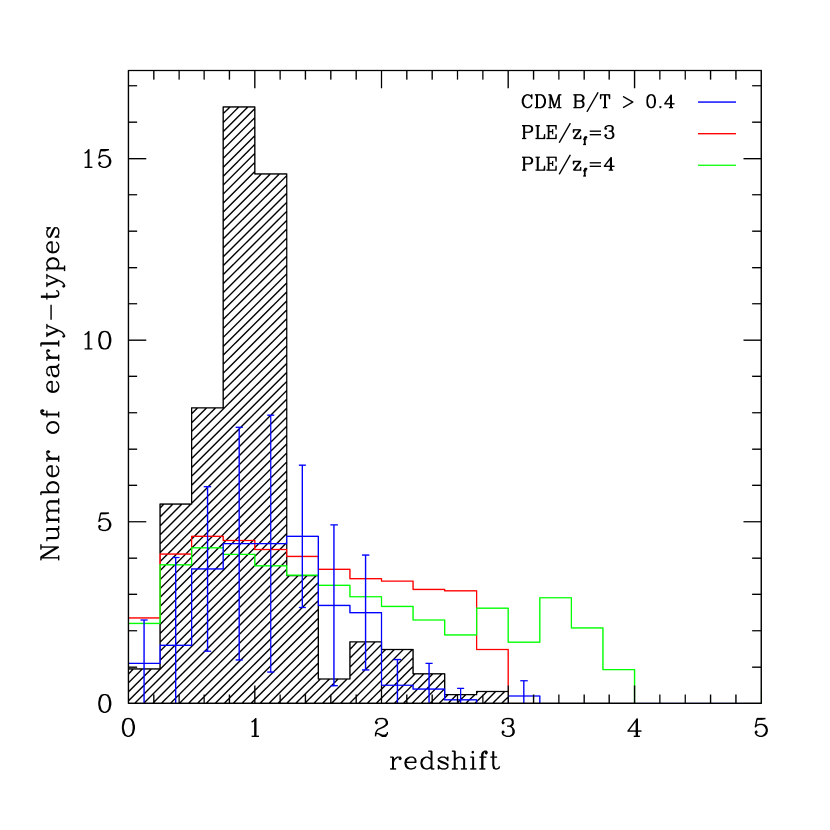
Figure 19: The number of early-types against redshift in the HNM at ${H_{160}}<24.0$ is shown by the shaded histogram. Two PLE model predictions are plotted based on the Marzke et al. local luminosity function: the red histogram has $z_{f}=3$ and the green histogram has $z_{f}=4$. The PLE models assume all stars are formed in a 0.1 Gyr burst with solar metallicity at the given $z_{f}$. The blue histogram shows a hierarchical merging prediction, along with scatterbars which show the one $\sigma$ variation to be expected due to large scale structure. The hierarchical merging model is described in Somerville et al. 2001. All model calculations assume $\Lambda=0.7,\Omega=0.3$, and $h=0.70$.

We have used the software described in Gardner (1980) to calculate the number of early-type galaxies which should be found in the HNM samples. These calculations primarily depend on a local luminosity function, the area and depth of the HNM sample, a galaxy evolution model, and a chosen cosmology. We use our standard Bruzual & Charlot PLE model to characterize the evolution of the early-type galaxies. We adopt the local luminosity function of early-type galaxies from Marzke et al. (1998). For early-type galaxies only, the relevant Schechter function parameters are $M_{B}^{*}=-20.15$, $\alpha=-1.0$, and $\phi^{*}=1.5\times 10^{-3}$ Mpc^-3. Clearly there are a large number of possible models which could be generated from the Gardner (1980) software to compare with the HNM primary and secondary samples, depending on e.g. the galaxy formation epoch and the cosmological parameters. Let us consider two simple examples with $z_{f}=3$ and $z_{f}=4$ in our default cosmology. These are shown in Figure 19 compared with the early-types that we have selected from the HNM. Neither of the two models based on the Marzke et al. local luminosity function provides a good description of the overall early-type redshift distribution. In particular, the observed early-type distribution has fewer galaxies at $z>1.5$ than the predictions.

To see how well the redshift distribution of the early-types could be matched by a hierarchical galaxy formation model, we used a simulation similar to that described in Somerville, Primack, & Faber (2001) and Firth et al. (2002). These simulations include modeling of the hierarchical build-up of structure, gas cooling, star formation and supernova feedback, galaxy mergers, chemical evolution, stellar populations and dust. Unlike the models presented in Somerville, Primack, & Faber (2001), here we have used the multi-metallicity stellar population models of Bruzual and Charlot (1998 version). Ten realizations were created and a single average mock object catalog was extracted from all the realizations so as to match the real $H<24.0$ catalog obtained from the HNM in terms of depth and area. From the mock catalog, we selected early-type galaxies by virtue of their having a bulge to total luminosity in the observed ${H_{160}}$ band greater than 0.4. While this selector appears to be a reasonable way to choose real early-type galaxies (Im et al., 2002), it is unclear how it relates to the visual method employed in selecting the primary and secondary early-type samples from the real data. The redshift distribution of the early-types morphologically selected from the hierarchical model is shown in Figure 19 by the blue histogram. The hierarchical prediction is a better match to the data at $z>1.5$ than the PLE models, but it also underpredicts the observed number of early-types at $z\sim 1$. Firth et al. (2002) found the similar result that the hierarchical models underpredict the number density of extremely red galaxies, which are believed to be early type galaxies at $z\sim 1$, compared to a larger-area ground-based sample selected at $H\lesssim 20$. The errorbars on the hierarchical model histogram give an indication of the scatter due to Poisson variation in the number of halos from realization to realization. The errorbars were determined by simply calculating the root mean square in the number of early-type galaxies at each redshift bin among the 10 realizations. They underestimate the expected scatter due to large scale structure, as the strong clustering of massive halos has not been accounted for.

The relative redshift distributions of the combined early-type samples, all of the galaxies at ${H_{160}}<24.0$, and all of the galaxies predicted by the CDM model to be at ${H_{160}}<24.0$ in the HDF-N are compared in Figure 20. This plot shows that the fraction of early-type galaxies in the total ${H_{160}}<24.0$ sample changes by only a small amount up to $z\sim 2$. But the comparison of the entire ${H_{160}}<24.0$ sample with all the galaxies in the hierarchical model indicates large changes in this ratio as a function of redshift.

Another approach to examining the space density evolution is to use the $\langle V/V_{max}\rangle$ statistic (Schmidt, 1968). This ratio is a measure of the position of a galaxy within the observable volume. In the case of constant space density, the individual values of the ratio will be uniformly distributed between 0 and 1, i.e. $\langle V/V_{max}\rangle=0.5$. The highest possible $z$ for each galaxy is calculated such that it would still be in the ${H_{160}}<24.0$ sample. The volume for this maximum redshift is $V_{max}$. The actual redshift of the galaxy gives the actual volume $V$. We made the $V_{max}$ calculation using our standard PLE model (making the galaxy brighter in the past) to estimate the upper redshift limit for a given galaxy. The result is shown in Figure 21 from which we calculate that $\langle V/V_{max}\rangle=0.31\pm 0.04$ for the combined primary+secondary samples. If only the primary sample was used, the resulting $\langle V/V_{max}\rangle=0.22\pm 0.05$. If we had assumed no-evolution in calculating $V_{max}$ then $\langle V/V_{max}\rangle=0.37\pm 0.04$ for all early-types.

Our analysis confirms previous findings (some of which based on the HDF-N) to the effect that the space density of early-type galaxies is substantially smaller at $z\gtrsim 1.4$ than at lower redshift (Zepf, 1997; Franceschini et al., 1998; Barger et al., 1999; Im et al., 1999; Menanteau et al., 1999; Abraham et al., 1999; Treu & Stiavelli, 1999). In the case of the HDF-N field, it is likely that no reasonable model can fit in detail the redshift distribution of not just the early-type but all galaxies due to the way that a large scale structure distorts the redshift distribution at $z\sim 1$. There are two well-known redshift spikes in the HDF-N galaxy distribution at $z=0.96$ and $z=1.02$ and both of these spikes are rich in early-type galaxies.

5.4 The Highest Redshift Early-type Galaxies?

While one of the main results of our study is the relative paucity of $z>1$ early-type galaxies in the HDF-N, there are two objects in our HNM catalog apparently at redshifts approaching $z\sim 2$ that seem to qualify as massive elliptical galaxies. Object # 731 is the host galaxy of SN 1997ff (Riess et al., 2001) and has a $z_{phot}=1.65$. A possible spectroscopic redshift of $z=1.755$ has been obtained as well (Riess et al., 2001). This object was classified as an elliptical by our visual inspection of its NIC3 image with an average T-type of $-3.3$, although with a significant spread in the assigned TT, and the surface brightness profile fitting gave a good fit to a de Vaucouleur law. In the rest frame, the galaxy is as red ($B-V=0.6$) and luminous ($M_{I}=-23.5$) at its redshift as expected for a massive, fully formed elliptical galaxy.

The second object which appears to be a high redshift early-type galaxy is #882 in our catalog with $z_{phot}=1.79$. It is quite close to #731 on the sky but not as well known and has not been the target of spectroscopy to determine its redshift. However, compared to #731, #882 has an even redder color and is similarly luminous in the rest frame $M(I_{814})$ band. Although the assigned T-type of $-3.3$ indicates that this object appears to be an elliptical based on its morphology in our NIC3 image, the profile fitting gave only a fair fit to a de Vaucouleur law. For both objects the SEDs indicate relatively little recent star formation, and the fitting in Dickinson, Papovich, & Ferguson (2003) gave masses of $\sim 10\times 10^{11}M_{\odot}$ which is very large given the high redshifts. Both of these objects are in our primary early-type sample.

6 Discussion

We have made a map of the HDF-N in the F110W and F160W filters using Camera 3 of the NICMOS onboard $HST$. Using these data, an object sample was selected from the F160W mosaic, which is $\sim$90% complete at ${H_{160}}_{AB}\sim 26.0$; here we reported results on the sample limited to ${H_{160}}_{AB}<24.0$. Hubble types were determined by visual inspection of the $H_{160}$ images. Galaxy spectral types were obtained from the procedure of estimating photometric redshifts. de Vaucouleur law profiles were fit to the $H_{160}$ surface brightness profiles and categorized by the goodness of the fit.

We have selected two samples of early-type galaxies. The primary sample consists of 34 galaxies with $-7<$ T-type $<-2$ and early-type galaxy spectral types. All these objects have fair or good $r^{1/4}$ law profile fits. The secondary sample of 42 galaxies has $-7<$ T-type $<0$, later-type galaxy spectral types, and fair or good $r^{1/4}$ law fits. The primary sample is more luminous (its average rest frame magnitude $M_{B}=-20.27$ vs $M_{B}=-19.4$ for the secondary sample) and generally physically larger at the same $M_{B}$ compared to the secondary one, independent of redshift. There are no major differences in the ${H_{160}}$ morphologies of the primary and secondary samples, and there is no difference in the nearby environments of the primary vs secondary samples of early-types, hence there is no evidence that the secondary sample is preferentially undergoing galaxy interactions. However the secondary sample is considerably bluer (rest frame $B-V=0.42$ on average vs $B-V=0.71$ for the primary sample), indicating that diffuse, widespread star formation has recently occurred in the secondary early-types. This would agree with the results of Trager et al. (2000) which show that $z=0$ ellipticals have a wide range of ages, from 1.5 Gyr up to a Hubble time. Also, the galaxies identified in our secondary sample may be similar to the ellipticals in the HDF which been shown to have blue cores and appear to be forming stars (Menenteau et al., 2001).

The relationship between the primary and secondary samples does not appear to be direct. Because they are blue and less luminous in the rest frame optical, the secondary galaxies are unlikely to evolve into the primary galaxies since they are less massive than the primary sample galaxies. After their current episodes of star formation end, the secondary galaxies will become redder but less luminous and their stellar masses will not increase. The secondaries could be the building blocks from which the primary galaxies are made through mergers. However their redshift distributions are broadly similar; one would expect there to be more secondaries at higher redshift in order to make the primaries that we see at $z<1.5$ in the HDF-N.

The redshift distribution of the early-type samples was examined to test the predictions of monolithic and hierarchical formation scenarios. Both the primary and secondary samples largely disappear at $z>1.4$; there are only a few early-types from the secondary sample up to $z\sim 2.5$. The observed redshift distribution does not match that predicted by a monolithic scenario. For a cosmology of $h=0.7$, $\Omega=0.3$, $\Lambda=0.7$, the predicted redshift distribution of passively evolving early-types formed at high redshift shows a deficit at $z\sim 1$ and an overabundance at $z>1.5$ with respect to the primary and to the primary+secondary samples in the HNM. A $V/V_{max}$ test agrees with this result. When the effects of passive luminosity evolution are included in the calculation, the mean value of $V_{max}$ for the primary sample is $0.22\pm 0.05$, and $0.31\pm 0.04$ for the combined primary+secondary sample. A hierarchical formation model such as that of Kauffmann, Charlot, & White (1996) or Somerville, Primack, & Faber (2001) better matches the overall redshift distribution of the early-types, with the exception of the spike at $z\sim 1$, though it still overpredicts the number at $z>1.5$.

Our results may be affected by several forms of bias. First, the apparently small number of early-types at $z>1$ could be due to a selection bias, if for example high redshift ellipticals are heavily obscured by dust during their formative stage. The SCUBA detections of high redshift galaxies indicates that this may be a real possibility, although the connection between the SCUBA sources and elliptical galaxies is still unknown. A more complicated situation would result if the progenitors of ellipticals galaxies are present at high redshift but we fail to select them because they are morphologically different from a present epoch elliptical. This could happen simply because the elliptical was undergoing a merger at the time of observation, or because there really is a morphological transformation from late-type to early-type which is the origin of present-epoch ellipticals. However, if ellipticals are morphologically different preferentially at $z>1$ and if they all form at the same time they should all (or nearly all) look morphologically similar at lower redshifts. The fact that we do not find the same density of ellipticals is a sign that there are multiple formation mechanisms and/or times for ellipticals. The fact that all nearby ellipticals have old stellar pops is a sign that the stars in ellipticals must exist at $z\sim 1.5$, but are not in what we can identify as ellipticals at that time. This would be an argument against the idea that monolithic collapse for some ellipticals happens later, at e.g. $z\sim 1$.

Previous studies of the N(z) of red and/or early-type galaxies have reported mixed results as to the number of such galaxies at $z>1$, as summarized in the Introduction. Field galaxy studies that use morphological identification of early-types tend to show a relatively small number at $z>1$ (Treu & Stiavelli, 1999; Benítez et al., 1999), while the larger area surveys that use only colors to identify early-types find a nearly constant space density (Cimatti et al., 2000; McCarthy et al., 2001). Our results on N(z) in the particular case of the HDF-N agree with previous studies (Zepf, 1997; Franceschini et al., 1998; Barger et al., 1999) in finding few morphologically-identified early-types at $z>1.5$. It is also true and perhaps significant that we find that there are not even many blue spheroidals at these higher redshifts, although there are a few at $2<z<3$. As for the complete disappearance of the red galaxies in the primary sample at $z>2$, the cause may be real morphological evolution which results in the higher redshift galaxies being left out of our morphological definition of an early-type sample (Conselice, 2003).

The HDF-N is one very small window on the universe. The N(z) of the early-type galaxies (indeed all galaxies in our sample) appears to be dominated by large scale structure at $z>0.8$; it seems impossible for any reasonable model to completely describe the observed N(z) of the HDF-N. Clearly, data similar to those employed here in terms of broad wavelength coverage, high resolution, and depth, but covering much larger areas are necessary to make further progress on the questions examined in this paper. The data from campaigns such as GOODS that are planned to probe the $z>1$ era over wider areas using e.g. ACS on HST, SIRTF, and DEIMOS at Keck and VIRMOS at the VLT should enable significantly better understanding of the origin and evolution of early-type field galaxies.

Figure 1: Average T-types vs $H_{160}$ for $H<24.0$ sample. Vertical bars represent the 1 $\sigma$ values on each average.

Figure 2: The difference TT($B_{r}$) - TT($H_{160}$) vs TT(H) for $H<24.0$ sample.

Figure 3: The difference TT($B_{r}$) - TT($H_{160}$) vs redshift for $H<24.0$ sample.

Figure 4: Average T-types vs redshift for $H<24.0$ sample. The upper $z$ limit is set by the available TT($B_{r}$).

Figure 5: $I-H$ vs $H_{160}$ for $H<24.0$ sample. The point symbol types denote the Hubble types as indicated in the legend. Objects with assigned T-types $<-7$ are termed as “compact”; these include stars. The diagonal dotted line indicates the 5 $\sigma$ limit in the color. The point size is inversely proportional to the redshift of the object, as indicated in the legend.

Figure 6: A plot of the $r_{e}$ determined by our profile fitting vs the input $r_{e}$ for two sets of model elliptical galaxies. The open squares represent models with ${H_{160}}=20.0$, the solid triangles those with ${H_{160}}=22.0$, and the open circles those with ${H_{160}}=24.0$. The points have been offset slightly in the horizontal direction for clarity. Errorbars representing one $\sigma$ are shown on each point.

Figure 7: Examples of the quality of $r^{1/4}$ law fits to the $H_{160}$ surface brightness profiles. In each plot, the object profile is represented by the solid square points with one $\sigma$ errorbars, the F160W PSF by a dotted line, and the best fitting $r^{1/4}$ law, convolved with the PSF, by a solid line. The object ID number, corresponding to the entries in Table 1, are shown in each panel. Here a good fit is shown.

Figure 7b: An example of a fair fit.

Figure 7c: An example of a poor fit.

Figure 8: Photometric vs spectroscopic redshifts where the latter are available. Morphologically-defined early and late-type galaxies are shown by different symbols. Errorbars are not shown to improve clarity since they are almost never larger than the points.

Figure 9: Galaxy spectral types, as determined from the photometric redshift procedure, vs T-types for HNM sample. The point style indicates the quality of the de Vaucouleur law fit to the object’s $H_{160}$ surface brightness profile, where a solid square is good, an open square is fair, and a $\times$ is poor. The dashed area in the shape of a square near the bottom shows the area of the primary early-type sample, and the dotted rectangle encloses the secondary sample of early-type galaxies, as described in the text.

Figure 10: Color composite images of the primary early-type sample. For each galaxy, $IJH$ images of a 10 arcsec area are shown on the right and $BVI$ images on the left. The redshifts are shown, with a p in parentheses to indicate the objects for which no spectroscopic redshift is available. The galaxy ID number is shown on the left.

Figure 10b: continued

Figure 11: Color composite images of the secondary early-type sample. For each galaxy, $IJH$ images of a 10 arcsec area are shown on the right and $BVI$ images on the left.The redshifts are shown, with a p in parentheses to indicate the objects for which no spectroscopic redshift is available. The galaxy ID number is shown on the left.

Figure 11b: continued

Figure 12: The rest frame $B-V$ color for the primary (solid squares) and secondary (open circles) samples of early-types against the asymetry index.

Figure 20: The relative numbers of all early-types against all galaxies at ${H_{160}}<24.0$ is shown by the solid line, and of all galaxies against the prediction of the CDM model for all galaxies in the ${H_{160}}<24.0$ sample.

Figure 21: A $V/V_{max}$ test for all early-types in the HNM sample at $H<24$.

Table 1: HNM ${H_{160}}<24.0$ Sample

ID	RA	Dec.	$H_{160}^{k}$	$I-H$	$z_{phot}$	$z_{spec}$	ST	TT	$\sigma$	$r_{e}$	$\mu_{e}$	q	$R_{e}$	$M_{{I_{814}}}$
			AB	AB						′′	mag/□′′		kpc	rest AB
32	12:36:46.91	62:14:22.1	19.47	0.47	0.140	0	0.970	-10.00	0.00	0.17	19.42	p	0.00	-11.78
40	12:36:48.63	62:14:23.2	23.52	0.48	0.946	-1	0.670	-8.00	2.94	1.37	27.36	p	10.46	-19.27
62	12:36:43.55	62:14:09.0	23.95	1.05	2.44	-1	0.710	3.00	3.63	0.11	21.77	p	0.89	-21.81
67	12:36:44.07	62:14:10.1	23.86	0.60	2.313	2.267	0.820	3.75	5.16	0.13	22.15	f	1.07	-20.88
108	12:36:52.80	62:14:32.1	20.69	0.18	0.431	0	0.590	-9.29	1.89	0.11	19.47	p	0.00	-10.84
109	12:36:48.23	62:14:18.5	23.49	0.74	2.244	2.009	0.740	5.20	3.83	0.29	23.33	f	2.43	-21.36
110	12:36:48.30	62:14:16.6	22.52	0.90	2.443	2.005	0.690	-3.00	2.45	0.17	21.40	f	1.42	-22.64
116	12:36:47.17	62:14:14.3	22.30	1.27	0.625	0.609	0.080	0.00	4.55	0.25	20.85	f	1.69	-19.62
121	12:36:44.85	62:14:06.1	23.14	1.57	1.9	-1	0.430	3.20	1.91	0.23	22.97	f	1.93	-22.05
133	12:36:48.09	62:14:14.5	23.95	0.61	0.92	-1	0.550	1.50	5.90	0.05	20.02	f	0.39	-19.23
143	12:36:46.48	62:14:07.6	23.05	0.41	0.599	0.13	0.750	2.40	5.55	1.99	27.36	p	4.62	-15.33
144	12:36:46.34	62:14:04.7	19.89	1.36	0.908	0.962	0.130	-3.14	2.55	0.59	21.78	g	4.68	-23.40
152	12:36:48.34	62:14:12.4	23.27	0.63	0.975	1.015	0.610	6.50	3.49	0.83	25.25	p	6.63	-19.97
154	12:36:50.35	62:14:18.7	22.66	0.49	0.815	0.819	0.570	2.21	1.82	1.03	25.25	p	7.80	-20.14
158	12:36:51.38	62:14:21.0	23.11	0.26	0.438	0.439	0.640	1.64	2.12	0.49	24.28	p	2.79	-18.18
161	12:36:49.57	62:14:14.8	23.61	0.48	0.953	-1	0.720	7.79	2.27	1.09	26.17	f	8.46	-19.30
163	12:36:49.82	62:14:14.8	22.44	1.29	1.366	1.98	0.440	5.14	2.39	1.67	25.61	f	13.99	-22.73
199	12:36:48.55	62:14:07.9	23.58	1.70	1.104	-1	0.130	-5.00	3.50	0.05	19.66	f	0.41	-20.00
214	12:36:49.50	62:14:06.8	20.76	1.04	0.843	0.752	0.260	-3.71	1.60	0.25	20.50	f	1.84	-21.83
215	12:36:46.03	62:13:56.4	23.30	0.92	0.914	-1	0.340	-1.42	2.76	0.17	22.15	f	1.34	-19.86
229	12:36:51.33	62:14:11.3	23.80	0.66	2.013	-1	0.800	4.00	7.84	0.21	22.90	p	1.75	-20.31
232	12:36:53.64	62:14:17.7	23.01	0.47	0.51	0.517	0.490	1.86	2.72	0.49	23.78	f	3.05	-18.67
257	12:36:51.39	62:14:08.2	23.80	1.51	1.204	-1	0.260	-3.40	2.06	0.17	22.83	f	1.43	-20.33
274	12:36:50.09	62:14:01.1	23.58	1.04	2.343	2.237	0.680	4.92	3.61	0.33	23.96	g	2.72	-22.10
282	12:36:53.58	62:14:10.2	23.97	0.53	3.432	3.181	0.720	6.10	2.94	0.35	24.28	p	2.65	-20.35
289	12:36:50.27	62:13:59.2	23.69	0.93	1.326	-1	0.670	0.70	3.31	0.23	23.33	p	1.92	-20.05
308	12:36:52.85	62:14:04.9	22.66	0.62	0.649	0.498	0.390	7.25	4.20	0.43	23.63	p	2.62	-18.91
313	12:36:51.97	62:14:00.9	22.35	0.71	0.54	0.559	0.370	1.50	2.55	0.77	23.70	p	4.98	-19.41
330	12:36:49.99	62:13:51.0	22.46	0.64	0.851	0.851	0.880	7.00	1.00	1.51	26.17	p	12.35	-20.94
331	12:36:49.42	62:13:46.9	17.51	0.68	0.093	0.089	0.000	-4.29	1.25	0.69	19.42	f	1.15	-19.89
333	12:36:47.17	62:13:41.9	22.62	1.07	1.268	1.313	0.530	-0.67	3.39	0.21	22.17	g	1.76	-21.36
340	12:36:51.78	62:13:53.9	20.03	1.08	0.541	0.557	0.160	1.36	1.97	0.59	21.67	p	3.81	-21.68
356	12:36:55.49	62:14:02.7	22.24	0.81	0.591	0.564	0.270	3.14	1.75	1.13	24.58	p	7.34	-19.53
359	12:36:42.03	62:13:21.4	23.59	0.40	0.936	0.846	0.620	-0.80	4.60	0.25	23.44	f	1.91	-19.37
360	12:36:52.74	62:13:54.8	21.47	0.53	1.28	1.355	0.740	9.60	0.55	1.95	25.61	p	16.42	-22.55
383	12:36:42.37	62:13:19.3	23.33	0.71	0.856	0.847	0.420	-6.00	3.00	0.07	20.47	f	0.54	-19.62
387	12:36:55.58	62:13:59.9	23.57	0.26	0.592	0.559	0.580	2.58	1.43	0.37	24.05	f	2.39	-18.30
388	12:36:54.09	62:13:54.4	21.69	0.80	0.836	0.851	0.390	-2.00	2.45	0.43	22.51	p	3.30	-21.23
402	12:36:52.22	62:13:48.1	23.90	0.46	0.57	-1	0.460	-2.60	3.50	0.07	21.05	f	0.45	-17.86
411	12:36:45.41	62:13:25.9	22.33	0.34	0.43	0.441	0.600	2.00	2.06	0.31	22.39	g	1.77	-19.03
412	12:36:45.86	62:13:25.8	20.37	0.58	0.424	0.321	0.430	3.29	1.38	1.99	24.58	p	9.27	-20.12
432	12:36:47.44	62:13:30.1	23.13	0.49	0.845	-1	0.940	0.25	4.51	0.51	24.42	p	3.93	-19.81
448	12:36:55.52	62:13:53.5	21.90	0.80	1.1	1.147	0.600	4.08	2.68	1.17	24.76	p	9.65	-21.78
457	12:36:54.77	62:13:50.8	23.57	0.64	0.845	-1	0.470	-0.30	2.86	0.23	23.13	f	1.77	-19.33
466	12:36:52.99	62:13:44.2	23.40	0.71	2.024	-1	0.770	9.50	0.50	0.43	24.42	f	3.58	-21.76
477	12:36:42.11	62:13:10.2	23.04	0.74	4.351	-1	0.540	-6.60	2.87	0.05	19.71	p	0.00	-23.41
488	12:36:48.57	62:13:28.3	22.34	0.63	0.85	0.958	0.460	3.86	2.91	1.19	24.97	p	9.44	-20.90
503	12:36:55.06	62:13:47.1	23.94	0.62	2.393	2.233	0.810	2.00	5.35	0.09	21.64	g	0.74	-21.54
519	12:36:42.52	62:13:05.2	23.57	0.79	1.097	-1	0.900	3.33	6.11	1.17	26.17	p	9.58	-19.97
520	12:36:42.72	62:13:07.1	21.03	1.23	0.666	0.485	0.050	-0.36	1.97	0.57	22.15	g	3.56	-20.50
522	12:36:44.10	62:13:10.8	22.96	1.07	3.041	2.929	0.550	7.20	3.56	0.45	23.50	p	3.50	-23.26
537	12:36:42.16	62:13:05.1	23.98	1.30	1.726	-1	0.520	5.30	3.83	0.13	22.27	f	1.10	-20.77
539	12:36:50.29	62:13:29.8	23.74	1.23	1.934	-1	0.640	2.30	3.31	0.21	23.38	p	1.76	-20.58
565	12:36:51.96	62:13:32.2	22.14	0.99	0.917	0.961	0.310	-5.00	1.15	0.17	21.33	f	1.34	-21.02
575	12:36:48.97	62:13:21.9	23.84	0.71	1.226	-1	0.860	-5.40	3.70	0.91	25.61	p	3.37	-15.86
576	12:36:49.07	62:13:21.9	22.54	1.81	1.078	-1	0.060	-0.29	3.08	0.41	22.93	g	3.29	-20.85
577	12:36:42.66	62:13:06.0	22.22	1.77	1.285	-1	0.190	3.58	1.74	1.73	24.97	p	14.67	-22.72
582	12:36:46.16	62:13:13.9	23.88	0.34	0.614	-1	0.620	-5.40	0.80	0.11	22.05	g	0.73	-18.11
604	12:36:44.76	62:13:07.0	23.95	0.64	2.776	-1	0.760	6.38	3.66	1.13	27.36	p	3.34	-14.46
605	12:36:44.58	62:13:04.6	20.01	1.24	0.449	0.485	0.050	3.29	1.68	1.17	22.64	p	7.03	-21.28
607	12:36:48.78	62:13:18.5	22.36	0.41	0.768	0.753	0.600	5.43	1.40	1.09	25.25	p	8.02	-20.26
608	12:36:48.46	62:13:16.7	22.53	0.78	0.502	0.474	0.250	-3.14	2.41	0.37	23.18	g	2.35	-19.18
609	12:36:48.26	62:13:13.8	22.11	1.80	1.158	-1	0.130	-3.29	1.25	0.51	23.44	g	4.12	-21.38
612	12:36:44.88	62:13:04.7	23.34	1.14	1.385	-1	0.540	-3.80	1.64	0.13	21.94	g	1.10	-20.92
613	12:36:46.74	62:13:12.3	23.25	0.35	0.599	-1	0.640	2.00	2.22	0.47	24.42	f	3.14	-18.80
614	12:36:45.62	62:13:08.8	23.08	0.57	0.508	-1	0.430	-3.71	2.63	0.29	23.33	g	1.78	-18.52
643	12:36:51.05	62:13:20.7	19.38	0.24	0.193	0.199	0.590	4.57	1.13	1.99	23.44	p	6.55	-20.11
653	12:36:56.64	62:13:39.9	23.87	1.42	1.783	-1	0.420	3.50	3.61	0.41	24.28	p	3.43	-21.68
659	12:36:49.46	62:13:16.7	21.72	1.50	1.243	1.238	0.290	4.00	1.29	0.61	23.18	f	5.09	-22.30
670	12:36:48.07	62:13:09.0	19.44	0.98	0.553	0.476	0.150	-5.71	1.89	0.63	21.61	f	3.74	-21.86
680	12:36:54.73	62:13:28.0	18.57	0.68	0.521	0	0.960	-9.71	0.76	0.25	19.53	p	0.00	-12.45
685	12:36:50.46	62:13:16.1	21.41	1.25	0.909	0.851	0.180	1.14	2.59	1.09	23.78	p	8.49	-21.64
700	12:36:49.03	62:13:09.8	23.62	0.41	0.856	-1	0.680	-2.00	2.55	0.22	23.11	f	1.66	-19.22
701	12:36:53.25	62:13:21.5	23.78	0.68	1.982	-1	0.790	1.30	2.49	0.29	23.96	f	2.42	-21.08
717	12:36:49.37	62:13:11.3	21.53	0.59	0.497	0.477	0.440	-5.00	0.00	0.19	20.85	f	1.13	-19.90
725	12:36:56.12	62:13:29.7	22.48	0.92	1.151	1.238	0.550	2.79	1.98	0.47	23.44	p	1.76	-17.09
731	12:36:44.11	62:12:44.8	21.58	2.83	1.661	1.755	0.060	-3.29	2.93	0.63	23.38	g	5.33	-23.51
732	12:36:44.43	62:12:44.1	23.27	0.74	1.982	-1	0.760	7.86	3.01	1.25	26.17	p	10.43	-21.66
734	12:36:43.97	62:12:50.1	20.02	1.01	0.511	0.557	0.190	2.64	1.52	1.61	22.80	p	10.40	-21.71
735	12:36:44.19	62:12:47.8	21.34	0.34	0.587	0.555	0.680	5.40	3.05	1.71	24.58	f	11.03	-20.54
741	12:36:53.18	62:13:22.7	23.99	0.90	2.636	2.489	0.720	-3.30	2.00	0.23	23.63	f	1.86	-21.69
748	12:36:38.60	62:12:33.8	23.76	0.34	0.425	0.904	0.590	1.58	2.94	0.39	24.05	f	2.17	-17.44
758	12:36:41.85	62:12:43.6	23.68	1.54	2.111	-1	0.480	4.58	2.82	0.61	25.25	p	5.01	-22.05
764	12:36:49.68	62:13:07.4	23.85	0.38	0.921	-1	0.690	-0.92	3.90	0.17	23.09	g	1.32	-19.19
775	12:36:49.71	62:13:13.1	20.40	1.07	0.452	0.475	0.140	-0.29	2.74	1.07	22.51	p	6.36	-20.83
779	12:36:38.41	62:12:31.3	21.47	1.26	0.516	0.944	0.050	0.79	2.75	0.97	23.50	p	6.07	-20.03
782	12:36:45.02	62:12:51.1	23.20	0.97	1.761	2.801	0.680	4.36	1.99	1.01	25.61	p	7.94	-22.85
784	12:36:56.13	62:13:25.2	22.66	2.42	1.316	-1	0.050	-5.00	0.00	0.11	21.01	g	0.93	-21.83
789	12:36:43.15	62:12:42.2	20.23	1.47	0.838	0.849	0.010	-4.71	0.76	0.31	20.66	g	2.37	-22.70
800	12:36:39.98	62:12:33.6	23.62	0.91	1.026	-1	0.460	0.75	2.44	0.15	22.27	g	1.21	-19.77
811	12:36:54.16	62:13:16.5	23.53	0.86	1.202	-1	0.630	-0.50	2.40	0.13	21.80	g	1.08	-20.22
813	12:36:47.72	62:12:55.8	23.64	0.98	3.024	2.931	0.610	7.42	2.73	0.95	25.61	p	7.38	-22.03
814	12:36:47.86	62:12:55.4	23.65	1.27	2.944	2.931	0.460	8.20	2.17	1.33	26.17	p	10.33	-22.60
819	12:36:55.02	62:13:18.8	23.75	1.41	0.849	-1	0.060	-4.00	1.26	0.17	22.93	g	1.30	-19.10
822	12:36:39.87	62:12:31.5	23.79	0.42	0.717	-1	0.460	1.08	2.75	0.17	22.59	g	1.22	-18.65
827	12:36:39.78	62:12:28.5	23.68	0.14	0.052	-1	0.800	6.10	3.72	1.33	26.17	p	3.46	-15.28
829	12:36:40.88	62:12:34.0	23.46	0.73	4.264	-1	0.520	-6.60	2.10	0.05	20.38	p	0.00	-23.26
833	12:36:45.98	62:12:50.4	23.96	0.45	3.809	-1	0.650	-6.60	2.10	0.05	20.58	p	0.00	-24.37
843	12:36:54.71	62:13:14.8	23.56	0.78	2.255	2.232	0.750	-2.30	3.90	0.17	22.64	g	1.40	-21.71
846	12:36:47.54	62:12:52.7	23.60	0.41	0.714	0.681	0.580	2.25	2.36	0.43	24.38	f	3.04	-18.75
847	12:36:46.13	62:12:46.5	21.16	1.20	0.765	0.9	0.070	-4.43	2.51	0.39	22.19	g	3.04	-21.94
848	12:36:54.99	62:13:14.8	23.71	0.18	0.536	0.511	0.640	-0.60	1.74	0.29	23.50	f	1.79	-17.98
855	12:36:49.63	62:12:57.6	20.92	1.09	0.456	0.475	0.160	-0.93	3.37	0.19	19.81	f	1.13	-20.35
860	12:36:44.18	62:12:40.4	22.98	0.35	0.888	0.875	0.660	6.71	1.89	1.73	26.17	p	13.37	-19.96
864	12:36:41.04	62:12:30.4	23.51	1.28	1.508	-1	0.490	6.50	1.66	0.63	25.25	f	5.34	-21.16
868	12:36:53.65	62:13:08.3	20.84	0.42	0.108	0	0.690	-9.29	1.89	0.11	19.67	p	0.00	-10.43
870	12:36:51.40	62:13:00.6	23.10	0.08	0.055	0.09	0.740	9.71	0.49	1.99	27.36	p	3.31	-14.49
880	12:36:48.32	62:12:49.8	19.83	1.11	0.726	0	1.000	-10.00	0.00	0.15	19.42	p	0.00	-10.76
882	12:36:45.66	62:12:41.9	22.27	3.28	1.792	-1	0.040	-3.29	2.98	0.21	21.86	f	1.77	-23.03
884	12:36:55.16	62:13:09.0	23.61	1.49	1.269	-1	0.300	2.12	3.79	0.53	24.76	p	4.46	-20.75
885	12:36:55.14	62:13:11.4	23.38	0.32	0.228	0.321	0.710	2.80	3.25	0.71	24.97	g	3.85	-17.76
886	12:36:55.45	62:13:11.2	20.44	1.75	0.973	0.968	0.020	-4.57	1.13	0.37	21.30	g	2.94	-22.86
893	12:36:38.98	62:12:19.7	21.68	0.57	0.623	0.609	0.450	3.50	3.71	1.57	24.76	p	10.58	-20.38
897	12:36:50.81	62:12:55.9	22.34	0.26	0.311	0.321	0.690	0.93	2.81	0.37	22.67	f	1.72	-18.26
909	12:36:57.73	62:13:15.2	22.24	0.64	0.843	0.952	0.550	8.21	2.51	1.11	24.97	p	8.79	-20.98
913	12:36:45.00	62:12:39.6	23.20	0.95	1.249	1.225	0.600	5.36	1.60	1.39	26.17	p	11.57	-20.70
921	12:36:49.46	62:12:48.8	23.13	0.83	0.678	-1	0.270	-3.50	2.60	0.17	22.21	g	1.20	-19.19
939	12:36:50.83	62:12:51.5	22.82	0.38	0.526	0.485	0.560	6.79	2.31	1.35	26.17	p	8.40	-18.84
942	12:36:48.99	62:12:45.9	23.50	0.29	0.484	0.512	0.580	3.80	5.40	0.71	24.97	f	4.23	-18.09
945	12:36:58.28	62:13:14.9	23.41	2.07	1.136	-1	0.050	-4.60	0.80	0.21	22.93	f	1.73	-20.28
953	12:36:54.18	62:13:01.1	23.78	1.19	1.197	-1	0.400	5.25	3.71	0.33	23.96	p	2.75	-20.09
954	12:36:46.77	62:12:37.1	21.61	0.78	0.708	0	0.980	-8.33	2.58	0.09	19.83	p	0.00	-9.28
955	12:36:47.04	62:12:36.9	20.59	0.47	0.432	0.321	0.530	-2.00	2.00	0.65	22.49	g	3.04	-19.94
956	12:36:55.15	62:13:03.6	21.97	1.60	0.905	0.952	0.030	-4.71	0.76	0.11	20.14	g	0.85	-21.07
971	12:36:50.26	62:12:45.8	20.19	1.22	0.753	0.68	0.080	-3.14	1.34	0.53	21.67	g	3.75	-22.09
972	12:36:39.72	62:12:14.1	22.31	1.61	0.989	-1	0.090	4.21	0.76	0.71	23.70	f	5.65	-20.96
975	12:36:57.21	62:13:07.7	22.55	2.03	1.102	-1	0.040	-5.83	2.04	0.09	20.37	g	0.74	-21.19
983	12:36:39.43	62:12:11.7	22.29	1.58	0.974	-1	0.080	-3.80	2.40	0.11	20.57	g	0.87	-20.95
989	12:36:44.64	62:12:27.4	22.61	1.16	1.444	2.5	0.520	0.30	4.06	0.31	22.83	f	2.50	-23.02
994	12:36:53.89	62:12:54.1	19.83	1.08	0.713	0.642	0.190	2.86	1.57	1.03	22.49	p	7.11	-22.28
1010	12:36:56.92	62:13:01.7	21.07	1.81	1.196	-1	0.140	-4.57	1.13	0.49	22.56	g	4.11	-23.09
1011	12:36:56.98	62:12:56.5	23.68	0.89	1.08	-1	0.520	4.12	1.51	0.71	25.61	f	5.83	-19.88
1014	12:36:41.49	62:12:15.0	21.63	1.83	1.024	-1	0.040	-2.33	2.29	0.11	19.74	f	0.88	-21.76
1021	12:36:46.21	62:12:28.5	23.74	1.08	1.453	-1	0.570	-0.40	7.90	0.61	25.25	p	5.16	-20.54
1022	12:36:50.22	62:12:39.8	20.17	0.52	0.478	0.474	0.460	6.10	1.85	1.99	23.70	p	11.81	-21.24
1023	12:36:47.78	62:12:32.9	22.40	0.96	0.941	0.96	0.350	-0.21	4.85	0.23	22.02	p	1.82	-20.85
1024	12:36:56.93	62:12:58.3	23.01	0.66	0.499	0.52	0.310	0.30	2.44	0.47	23.70	f	2.93	-18.61
1027	12:36:42.92	62:12:16.3	20.11	0.64	0.45	0.454	0.390	3.36	1.80	1.99	23.63	p	11.53	-21.18
1029	12:36:47.28	62:12:30.7	22.45	0.36	0.446	0.421	0.580	3.29	2.67	0.51	23.63	f	2.83	-18.74
1031	12:36:40.01	62:12:07.3	20.91	1.39	0.887	1.015	0.100	-4.00	2.24	0.29	21.27	f	2.33	-22.51
1036	12:36:43.63	62:12:18.3	22.22	0.53	0.761	0.752	0.490	-0.86	3.81	0.35	22.80	f	2.57	-20.41
1042	12:36:57.30	62:12:59.7	21.07	0.29	0.492	0.475	0.640	3.90	2.09	1.91	24.76	f	11.34	-20.37
1047	12:36:49.56	62:12:36.0	23.48	1.18	1.993	-1	0.620	1.20	0.45	0.21	22.76	f	1.75	-21.76
1050	12:36:56.57	62:12:57.4	23.31	2.31	1.197	-1	0.030	-5.00	1.90	0.05	19.95	f	0.42	-20.90
1051	12:36:58.06	62:13:00.4	22.12	0.27	0.321	0.32	0.710	0.50	2.90	0.31	22.25	f	1.45	-18.45
1076	12:36:40.84	62:12:03.1	22.61	0.61	0.984	1.01	0.640	9.60	0.49	0.79	24.42	f	6.35	-20.73
1077	12:36:40.75	62:12:04.9	23.56	1.06	0.919	-1	0.260	-0.50	3.50	0.17	22.67	g	1.33	-19.57
1078	12:36:40.96	62:12:05.3	22.52	0.78	2.666	0.882	0.680	-6.25	2.16	0.07	19.98	f	0.56	-22.35
1080	12:36:54.04	62:12:45.6	22.00	0.74	0.762	0	0.990	-5.83	3.44	0.07	19.52	p	0.00	-8.96
1086	12:36:55.61	62:12:49.2	22.67	0.41	0.903	0.95	0.650	7.08	2.84	1.63	26.17	p	12.90	-20.46
1087	12:36:55.24	62:12:52.5	23.94	0.33	0.699	-1	0.730	8.36	2.84	0.83	26.17	p	5.79	-18.28
1090	12:36:56.60	62:12:52.7	23.52	0.82	1.27	1.231	0.740	2.40	6.10	1.99	26.17	p	16.59	-20.27
1091	12:36:56.72	62:12:52.6	21.77	1.98	1.219	-1	0.110	-3.86	2.27	0.31	22.21	f	2.58	-22.24
1092	12:36:44.56	62:12:15.5	23.06	2.32	1.751	-1	0.140	5.00	4.55	0.69	24.76	p	5.81	-22.45
1115	12:36:41.26	62:12:03.0	23.89	0.49	3.226	3.216	0.750	8.75	2.60	1.03	26.17	p	7.77	-23.58
1117	12:36:41.95	62:12:05.4	20.22	0.78	0.459	0.432	0.310	-1.00	2.77	0.61	21.78	p	3.44	-20.90
1120	12:36:55.56	62:12:45.5	21.08	0.90	0.785	0.79	0.300	-3.86	2.04	0.33	21.73	f	2.47	-21.65
1127	12:36:56.64	62:12:45.5	18.94	1.05	0.589	0.518	0.150	2.57	1.62	1.99	22.67	p	12.40	-22.57
1128	12:36:45.42	62:12:13.6	22.12	-0.98	0.000	0	0.950	-8.00	3.46	0.07	19.89	p	0.00	-10.57
1135	12:36:59.30	62:12:55.8	21.53	0.95	0.764	0	1.000	-7.83	2.27	0.07	19.42	p	0.00	-9.21
1136	12:36:58.76	62:12:52.4	20.89	0.40	0.422	0.321	0.540	3.86	1.22	1.99	24.76	f	9.29	-19.61
1141	12:36:49.98	62:12:26.3	23.69	0.86	1.234	-1	0.650	2.10	4.56	0.55	24.58	p	4.53	-20.64
1160	12:36:50.84	62:12:27.2	23.82	0.46	0.707	-1	0.500	5.58	3.32	0.47	24.97	f	3.36	-18.58
1166	12:36:49.95	62:12:25.5	23.26	1.10	1.234	1.205	0.490	-5.00	0.00	0.09	21.16	g	0.35	-16.41
1168	12:36:49.06	62:12:21.2	21.86	0.62	0.915	0.953	0.550	5.10	3.29	0.45	23.13	p	3.56	-21.37
1171	12:36:53.44	62:12:34.3	22.18	0.67	0.576	0.56	0.410	1.57	2.28	0.43	22.73	p	2.79	-19.60
1198	12:36:49.53	62:12:20.1	23.91	0.56	0.94	0.961	0.620	1.17	2.21	0.41	24.28	p	3.25	-19.35
1208	12:36:52.86	62:12:29.6	23.73	0.89	0.701	-1	0.220	2.43	1.24	0.47	24.76	g	3.37	-18.64
1211	12:36:48.63	62:12:15.8	22.16	2.38	1.711	-1	0.120	-1.29	2.98	0.29	22.35	g	2.44	-23.33
1213	12:36:48.25	62:12:13.8	21.75	0.85	0.949	0.962	0.430	4.57	1.13	1.99	25.61	p	15.80	-21.45
1214	12:36:52.09	62:12:26.3	21.83	2.03	1.119	-1	0.040	-3.80	2.40	0.26	22.00	g	2.11	-21.71
1229	12:37:00.11	62:12:49.9	23.37	1.07	1.291	-1	0.560	-1.50	3.32	0.09	21.12	g	0.75	-20.46
1231	12:36:55.03	62:12:34.2	22.38	1.87	1.108	-1	0.080	0.25	3.03	0.11	20.29	g	0.91	-21.40
1240	12:36:50.16	62:12:17.0	20.96	1.48	0.908	0.905	0.070	2.50	2.71	0.49	21.99	f	3.80	-22.08
1247	12:36:56.35	62:12:41.1	19.02	0.25	0.000	0	0.340	-9.29	1.89	0.21	19.42	p	0.00	-12.43
1253	12:36:51.71	62:12:20.2	20.69	0.89	0.43	0.401	0.230	-0.64	2.69	0.47	21.43	f	2.53	-20.19
1258	12:36:44.83	62:12:00.2	22.62	0.43	0.487	0.457	0.530	3.58	2.05	1.35	25.61	f	7.85	-18.74
1266	12:36:46.41	62:12:04.6	23.94	0.70	1.175	-1	0.810	9.33	1.21	1.95	27.36	p	14.84	-18.68
1282	12:36:46.95	62:12:05.3	23.87	0.24	0.051	-1	0.640	4.37	1.85	0.35	24.42	f	1.95	-17.35
1286	12:36:45.96	62:12:01.4	23.29	0.48	0.733	0.679	0.540	1.00	2.36	0.43	23.96	f	3.04	-19.10
1305	12:36:53.42	62:12:21.7	23.69	0.35	1.877	-1	0.850	5.25	2.95	0.35	24.28	f	2.93	-21.49
1315	12:36:51.61	62:12:17.3	23.81	1.24	1.945	-1	0.510	-2.00	2.55	0.07	20.90	g	0.58	-21.62
1316	12:36:43.42	62:11:51.5	22.37	0.67	1.191	1.242	0.750	-3.33	2.62	0.13	20.82	g	1.08	-21.54
1325	12:36:52.67	62:12:19.7	22.81	0.42	0.46	0.401	0.550	-3.20	1.47	0.15	21.37	f	0.81	-18.27
1335	12:36:41.41	62:11:42.5	21.04	1.93	1.499	1.524	0.220	4.50	1.32	1.93	24.58	p	16.32	-24.13
1336	12:36:41.32	62:11:40.8	21.47	1.32	0.651	0.585	0.050	-2.64	2.87	0.45	22.29	f	2.98	-20.35
1348	12:36:43.19	62:11:48.0	20.75	1.69	1.022	1.01	0.080	-0.29	2.75	0.71	22.76	p	5.70	-22.66
1354	12:36:45.06	62:11:54.1	23.55	0.65	0.879	-1	0.930	2.38	5.76	1.07	26.17	f	8.27	-19.36
1355	12:36:45.66	62:11:53.9	23.07	1.35	1.157	-1	0.320	-1.00	2.12	0.19	22.42	g	1.57	-20.66
1356	12:36:45.33	62:11:54.5	21.33	1.78	1.015	-1	0.050	-3.67	1.97	0.31	21.77	g	2.48	-22.03
1357	12:36:45.41	62:11:53.1	23.21	0.93	3.028	2.803	0.620	-0.90	3.54	0.99	25.25	f	7.78	-22.81
1358	12:36:45.30	62:11:52.2	23.49	0.63	3.017	2.803	0.740	7.92	2.91	0.97	25.25	f	7.62	-22.83
1359	12:36:49.31	62:12:07.3	23.76	1.07	0.921	-1	0.250	0.60	2.48	0.19	22.80	f	1.49	-19.36
1364	12:36:42.15	62:11:44.7	23.82	0.72	1.506	-1	0.790	6.50	4.05	0.33	24.28	f	2.79	-19.93
1411	12:36:52.01	62:12:09.7	22.59	0.33	0.506	0.458	0.600	-0.83	3.29	0.83	24.97	g	4.83	-18.80
1414	12:36:57.20	62:12:25.8	22.03	0.42	0.616	0.561	0.600	2.75	1.37	0.71	24.28	p	4.60	-19.83
1418	12:36:43.81	62:11:42.8	19.56	1.29	0.763	0.765	0.030	-5.00	0.00	0.61	21.46	g	4.51	-23.07
1429	12:37:00.56	62:12:34.7	20.42	0.98	0.577	0.563	0.130	-5.71	1.89	0.33	21.10	g	2.14	-21.39
1434	12:36:46.52	62:11:51.3	20.97	1.02	0.546	0.503	0.130	-4.71	0.76	0.11	19.42	g	0.68	-20.53
1436	12:36:54.78	62:12:16.6	23.58	0.80	1.742	-1	0.740	3.42	0.97	0.45	24.16	f	3.77	-20.94
1446	12:36:44.49	62:11:43.7	23.79	0.47	0.98	1.02	0.730	10.00	0.00	1.13	26.17	p	9.10	-19.55
1447	12:36:44.46	62:11:41.6	22.52	0.62	0.967	1.02	0.610	5.86	2.46	1.91	26.17	p	15.38	-20.87
1453	12:36:56.64	62:12:20.1	20.91	1.57	0.933	0.93	0.060	-3.00	2.52	0.37	21.80	f	2.90	-22.21
1462	12:36:41.63	62:11:31.8	19.64	0.18	0.083	0.089	0.740	2.00	1.55	1.99	23.44	p	3.31	-18.13
1469	12:36:42.30	62:11:34.7	23.16	0.81	0.753	-1	0.330	2.50	2.10	0.61	24.76	f	4.53	-19.40
1474	12:36:47.45	62:11:50.8	23.49	0.59	0.884	-1	0.500	0.83	2.54	0.13	21.67	f	1.01	-19.55
1481	12:36:45.31	62:11:42.8	23.78	0.20	0.66	0.558	0.700	6.83	4.17	0.33	23.87	p	2.13	-18.08
1482	12:36:49.35	62:11:55.0	23.24	0.24	0.998	0.961	0.800	-3.20	1.83	0.05	19.53	f	0.40	-20.02
1486	12:36:55.37	62:12:13.4	23.71	0.97	4.611	-1	0.410	-6.60	2.10	0.13	22.39	p	0.85	-23.14
1488	12:36:46.18	62:11:42.1	19.88	1.42	1.088	1.013	0.230	3.71	1.11	1.97	23.70	p	15.85	-23.55
1495	12:36:46.87	62:11:44.9	22.57	0.74	1.072	1.06	0.660	4.00	1.53	1.79	26.17	p	14.54	-20.83
1510	12:36:58.64	62:12:21.7	23.00	0.42	0.71	0.682	0.610	-4.80	3.03	0.15	21.75	f	1.06	-19.38
1512	12:36:52.10	62:12:01.2	23.48	2.76	1.534	-1	0.060	6.75	3.46	0.77	25.61	f	6.53	-21.22
1513	12:37:00.07	62:12:25.3	23.06	0.77	2.379	2.05	0.740	6.30	2.96	0.41	23.78	p	3.35	-21.80
1521	12:36:52.56	62:12:01.6	23.24	0.30	0.465	-1	0.480	-1.00	6.16	0.19	22.70	f	1.14	-18.34
1522	12:36:43.90	62:11:34.1	22.71	1.83	1.028	-1	0.050	-5.00	0.00	0.05	19.56	g	0.40	-20.65
1523	12:36:44.39	62:11:33.1	19.34	1.99	1.038	1.05	0.010	-5.00	0.00	0.85	21.87	g	6.83	-24.10
1525	12:36:49.25	62:11:48.5	21.61	1.37	0.975	0.961	0.170	-3.67	2.21	0.37	22.08	f	2.94	-21.65
1538	12:36:55.95	62:12:10.7	23.41	1.16	1.312	-1	0.470	-4.50	1.00	0.23	23.13	g	1.94	-20.76
1550	12:36:58.29	62:12:16.5	23.75	1.50	2.14	-1	0.470	0.60	4.30	0.15	22.46	f	1.23	-21.99
1553	12:37:01.65	62:12:25.9	23.57	0.27	0.929	0.973	0.780	6.80	3.70	0.41	24.28	f	3.27	-19.48
1558	12:36:44.75	62:11:33.4	22.65	1.80	0.913	-1	0.000	-6.00	2.24	0.07	20.39	f	0.55	-20.59
1562	12:36:57.58	62:12:12.7	23.44	0.33	0.796	0.561	0.520	6.80	3.27	1.57	26.17	p	11.83	-19.38
1563	12:36:57.48	62:12:10.6	19.77	1.29	0.858	0.665	0.070	-3.43	2.30	0.41	20.79	g	2.87	-22.44
1564	12:36:51.96	62:11:55.4	23.52	0.27	0.426	-1	0.530	5.40	2.30	1.05	26.17	p	5.93	-17.55
1568	12:36:54.38	62:12:02.6	23.33	1.39	1.233	-1	0.320	6.80	3.27	0.15	21.90	f	1.26	-20.72
1569	12:36:56.42	62:12:09.3	23.08	0.29	0.398	0.321	0.620	3.67	2.48	0.93	24.97	p	4.34	-17.60
1578	12:36:58.30	62:12:14.2	22.96	0.40	0.987	1.020	0.710	-1.50	3.54	0.17	22.08	g	1.37	-20.40
1582	12:36:49.12	62:11:50.6	23.85	1.52	1.504	-1	0.370	0.12	3.71	0.23	23.23	g	1.95	-21.03
1594	12:37:01.71	62:12:23.6	23.79	0.48	1.114	1.191	0.760	-5.40	3.70	0.19	22.86	f	1.55	-19.69

References

- Abraham et al. (1999) Abraham, R. G., Ellis, R. S., Fabian, A. C., Tanvir, N. R., Glazebrook, K. 1999, MNRAS, 303, 641
- Barger et al. (1999) Barger, A.J., Cowie, L.L., Trentham, M., Fulton, E., Hu, E.M., Songaila, A., & Hall, D. 1999, AJ, 117, 102
- Benítez et al. (1999) Benítez, N., Broadhurst, T., Bouwens, R., Silk, J. & Rosati, P. 1999, ApJ, 515, L65
- Bertin & Arnouts (1996) Bertin, E. & Arnouts, S. 1996, A&AS, 117, 393
- Blanton et al. (2001) Blanton, M. et al. 2001, AJ, 121, 2358
- Brinchmann et al. (1998) Brinchmann, J. et al. 1998, ApJ, 499, 112
- Budavári et al. (2000) Budavári, T., Szalay, A.S., Connolly, A.J., Csabai, I., & Dickinson, M. 2000, AJ, 120, 1588
- Cimatti et al. (2000) Cimatti, A. et al. 2000, A&A, 361, 535
- Cohen et al. (2000) Cohen, J.G., Hogg, D., Blandford, R., Cowie, L., Hu, E., Songaila, A., Shopbell, P., & Richberg, K. 2000, ApJ, 538, 29
- Cohen (2001) Cohen, J.G. 2001, AJ, 121, 2895
- Coleman, Wu, & Weedman (1980) Coleman, G.D., Wu, C.-C., & Weedman, D.W. 1980, ApJS, 43, 393
- Conselice (2003) Conselice, C.J. 2003, ApJS, in press
- Daddi et al. (2000) Daddi, E., Cimatti, A., & Renzini, A. 2000, A&A, 362, 45
- Daddi et al. (2001) Daddi, E., Broadhurst, T., Zamorani, G., Cimatti, A., R ttgering, H., Renzini, A. 2001, A&A, 376, 825
- Dawson et al. (2001) Dawson, S., Stern, D., Bunker, A., Spinrad, H., & Dey, A. 2001, AJ, 122, 598
- Dickinson (1998) Dickinson, M. 1998, in “The Hubble Deep Field”, eds. M. Livio, S.M. Fall, & P. Madau (Cambridge: Cambridge University Press), p. 219
- Dickinson, Papovich, & Ferguson (2003) Dickinson, M., Papovich, C., Ferguson, H.C., & Budavari, T. 2003, ApJ, in press
- Driver et al. (1998) Driver, S.P., Fernandez-Soto, A., Couch, W.J., Odewahn, S.C., Windhorst, R.A., Phillips, S., Lanzetta, K., & Yahil, A. 1998, ApJ, 496, L93
- Eggen, Lynden-Bell, & Sandage (1962) Eggen, O.J., Lynden-Bell, D., Sandage, A.R. 1962, ApJ, 136, 748.
- Fernandez-Soto, Lanzetta, & Yahil (1999) Fernandez-Soto, A., Lanzetta, K.M., & Yahil, A. 1999, ApJ, 513, 34
- Firth et al. (2002) Firth, A.E. et al. 2002, MNRAS, 332, 617
- Franceschini et al. (1998) Franceschini, A. et al. 1998, ApJ, 506, 600
- Frei et al. (1996) Frei, Z., Guhathakurta, P., Gunn, J.E., & Tyson, J.A. 1996, AJ, 111, 174
- Fruchter & Hook (2002) Fruchter, A. & Hook, R. 2002, PASP, 114, 144
- Gardner (1980) Gardner, J. 1998, PASP, 110, 291
- Im et al. (1999) Im, M., Griffiths, R.E., Naim, A., Ratnatunga, K.U., Roche, N., Green, R.F., & Sarajedini, V.L. 1999, ApJ, 510, 82
- Im et al. (2001) Im, M., et al. 2001, AJ, 122, 750
- Im et al. (2002) Im, M. et al. 2002, ApJ, 571, 136
- Jorgensen, Franx, & Kjaergaard (1996) Jorgensen, I., Franx, M., & Kjaergaard, P. 1996, MNRAS, 280, 167
- Kauffmann, Charlot, & White (1996) Kauffmann, G., Charlot, S., & White, S. 1996, MNRAS, 283, L117
- Kron (1980) Kron, R. 1980, ApJS, 43, 305
- Lilly et al. (1995) Lilly, S.J., Tresse, L., Hammer, F., Crampton, D., & Le Fevre, O. 1995, ApJ, 455, 108
- Marzke et al. (1998) Marzke, R., da Costa, L.N., Pellegrini, P.S., Willmer, C.N.A., & Geller, M. 1998, ApJ, 503, 617
- McCarthy et al. (2001) McCarthy, P.J., et al. 2001, ApJ, 560, L131
- McCracken et al. (2000) McCracken, H., Metcalfe, N., Shanks, T., Campos, A., Gardner, J. P., & Fong, R. 2000, MNRAS, 311, 707
- Menanteau et al. (1999) Menanteau, F., Ellis, R.S., Abraham, R.G., Barger, A.J., & Cowie, L.L. 1999, MNRAS, 309, 208
- Menenteau et al. (2001) Menanteau, F., Abraham, R.G., & Ellis, R.S. 2001, MNRAS, 322, 1