Experimental Limit on the Cosmic Diffuse Ultra-high Energy Neutrino Flux

Abstract

We report results from 120 hours of livetime with the Goldstone Lunar Ultra-high energy neutrino Experiment (GLUE). The experiment searches for $\leq 10$ ns microwave pulses from the lunar regolith, appearing in coincidence at two large radio telescopes separated by 22 km and linked by optical fiber. Such pulses would arise from subsurface electromagnetic cascades induced by interactions of $\geq 100$ EeV neutrinos in the lunar regolith. No candidates are yet seen, and the implied limits constrain several current models for ultra-high energy neutrino fluxes.

In 1962, G. Askaryan predicted that electromagnetic cascades in dense media should produce strong coherent pulses of microwave Cherenkov radiation Ask62 . Recent confirmation of this hypothesis at accelerators Sal01 strengthens the motivation to search for such emission from cascades induced by predicted high energy neutrino fluxes, closely related to the measured fluence of $\simeq 10^{20}$ eV cosmic rays in many models.

Two such models, the Z-burst model Wei99 , and a generic class known as Topological Defect (TD) models Yos97 , predict ultra-high energy (UHE) neutrinos with either monoenergetic or very hard energy spectra. In the Z-burst model, UHE neutrinos annihilate with relic cosmic background neutrinos via the $\nu\bar{\nu}\rightarrow Z_{0}$ channel. The $Z_{0}$ then decays rapidly in a burst of hadronic secondaries which create the observed $\sim 10^{20}$ eV cosmic rays. The need to match the observed UHE cosmic ray fluxes and satisfy the current constraints on neutrino masses (which modify the annihilation resonance energy) then lead to a requirement on minimal neutrino fluxes at the resonance energy near $10^{22-23}$ eV. The Z-burst model thus formally requires only neutrinos at a single energy, with no specification for how such a flux might be produced.

The Z-burst model is also significant in that it is a variation on an earlier idea Weiler82 in which the $\nu\bar{\nu}$ annihiliation process could be used as a probe of the cosmic background neutrinos, one of the few viable ways ever proposed for detection of these relic cosmological neutrinos–it requires only a sufficient flux of UHE neutrinos and a detector with the sensitivity to measure them. Constraints on these UHE $\nu$ fluxes thus can rule out this potential detection channel for the relics, in addition to excluding their role in UHE cosmic ray production.

TD models, in contrast, postulate a very massive relic particle from the early universe which is decaying in the current epoch and producing secondaries observed as UHE cosmic rays. The required masses approach the Grand-Unified Theory (GUT) scale at $\sim 10^{24}$ eV, and the decay products thus have a very hard spectrum extending up to the rest mass energy of the particles. Because of these very hard spectra, detectors optimized for lower-energy neutrinos, even up to PeV energies, do not yet constrain these models, and new approaches, such as the experiment we report on here, are required.

Neutrinos with energies above 100 EeV (1 EeV = $10^{18}$ eV) can produce cascades in the upper 10 m of the lunar regolith resulting in pulses that are detectable at Earth by large radio telescopes. Zhe88 ; Dag89 One prior experiment has been reported, using the Parkes 64 m telescope H96 with 10 hours of livetime. In the decimeter band, the signal should appear as highly linearly-polarized, band-limited electromagnetic impulses zhsa . However, since there are many anthropogenic sources of impulsive radio-frequency interference (RFI), the primary problem in detecting neutrinos is to reject such interference. Since 1999 we have conducted a series of experiments in search of such pulses, using the JPL/NASA Deep Space Network antennas at Goldstone, CA Gor99 . We have essentially eliminated RFI background by employing two antennas in coincidence.

Although the total livetime accumulated in our experiment is a relatively small fraction of what is possible with a dedicated system, the volume of material to which we are sensitive is enormous, exceeding 100,000 km³ at the highest energies. The resulting sensitivity is enough to begin constraining some models for diffuse neutrino fluxes at energies above $10^{20}$ eV. We report here on results from 120 hours of livetime.

The lunar regolith is an aggregate layer of fine particles and small rocks, consisting mostly of silicates and related minerals, with meteoritic iron and titanium compounds at an average level of several per cent, and traces of meteoritic carbon. Its depths are 10 to 20 m in the maria and valleys, but may be hundreds of meters in portions of the highlands Mor87 . It has a mean dielectric constant of $\epsilon=n^{2}\simeq 3$ and a density of $\rho\simeq 1.7$ g cm^-3, both increasing slowly with depth. Measured values for the loss tangent vary widely depending on iron and titanium content, but a mean value at high frequencies is $\tan\delta\simeq 0.003$, implying a field attenuation length $L_{\alpha}\simeq~{}9$ m at 2 GHz Olh75 .

Fig. 1 illustrates the signal emission geometry. At 100 EeV the interaction length of a neutrino is about 60 km Gan00 . Upon interaction, a cascade $\sim 10$ m long forms, and Compton scattering, positron annihilation, and other processes lead to a $\sim 20\%$ negative charge excess. This cascade radiates a cone of coherent Cherenkov emission at an angle from the shower axis of $\theta_{C}=\cos^{-1}(1/\beta\sqrt{\epsilon})\simeq 54^{\circ}$, with an angular spread of $\Delta\theta\simeq 1^{\circ}$ at 2 GHz. At an ideal smooth regolith surface, the refraction obeys Snell’s law, and the exit angle $\theta^{\prime}$ is magnified by the gradient $\Delta\theta^{\prime}/\Delta\theta=n\cos\theta/\sqrt{1-n^{2}\sin^{2}\theta}$ which equals $n$ for normal incidence ($\theta=0$), but becomes much larger as $\theta$ approaches the total-internal reflectance angle $\theta_{TIR}=\pi/2-\theta_{C}$. This magnification improves the acceptance for an earth-based detector, at the expense of an increase in energy threshold. Our ray tracing shows that similar effects obtain statistically for a more realistic surface as well.

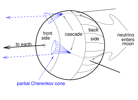
Figure 1: Geometry of lunar neutrino cascade event detection.

For our search we used the shaped-Cassegrainian 70 m antenna DSS14, and the 34 m beam-waveguide antenna DSS13, separated by 22 km. The S-band (2.2 GHz) right-circular-polarization (RCP) signal from DSS13 is filtered to 150 MHz bandwidth and down-converted to an intermediate frequency (IF) near 300 MHz. The band is subdivided into high and low frequency halves with no overlap. The DSS14 dual polarization S-band signals are down-converted to the same 300 MHz IF, and a combination of bandwidths from 40-150 MHz are used for sub-band triggering on impulsive signals. At DSS14, an L-band (1.8 GHz) feed which is off-pointed by $\sim 0.5^{\circ}$ produces a 40 MHz bandwith monitor of terrestrial interference signals.

Fig. 2 shows the layout of the trigger. The signals from the two antennas are converted to unipolar pulses using tunnel-diode detectors with a $\sim 10$ ns integration time. A comparator then test for pulses above threshold, and a local coincidence within 50 ns is formed among the channels at each antenna. The DSS14 coincidence between both circular polarizations ensures that the signals are highly linearly polarized, and the split-channel coincidences ensure that the signal is broadband.

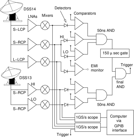
Figure 2: GLUE trigger and data recording system.

A global trigger is formed between the local coincidences of the two antennas within a 150 $\mu$s window, which encompasses the possible geometric delay range for the Moon throughout the year. Although use of a smaller window is possible, a tighter coincidence is applied offline and the out-of-time events provide a large background sample. Upon the global coincidence, a 250 $\mu$s record, sampled at 1 Gsamples/s, is stored. The average trigger rate, due primarily to random coincidences of thermal noise fluctuations, is $3\times 10^{-3}$ Hz. Terrestrial interference triggers are on average a few percent of the total, but we have averaged $\geq 95$% livetime during the runs to date.

The precise geometry of the experiment is a crucial discriminator for events from the Moon. The relative delay between the two antennas is $\tau=c^{-1}|\vec{B}|\cos\theta$ where $\theta$ is the apparent angle of the Moon with respect to the baseline vector, $\vec{B}$. For our 22 km baseline, we have a maximum delay difference of $\tau_{max}=\pm 73~{}\mu$s. Detectable events can occur anywhere on the Moon’s surface within the antenna beam. This produces a possible spread of 630 ns in the differential delay of the received pulses at the two antennas.

The 2.2 GHz antenna beamwidths between the measured first Airy nulls are $0.27^{\circ}$ for the 70 m, and $0.56^{\circ}$ for the 34 m. We took data in three configurations: pointing at the limb, the center, and halfway between. The measured source temperatures varied from 70K at the limb, to 160K at the Moon center, with system temperatures of 30-40K.

Timing and amplitude calibration are accomplished in several steps. We internally calibrate the back-end trigger system using a synthesized IF pulse signal, giving precision of order 1 ns. We use a pulse transmitter (single-cycle at 2.2GHz) aimed at the antennas to calibrate the cross-channel delays of each antenna to a precision of 1 ns. The cross-polarization timing at DSS 14 is also checked since the thermal radiation from the limb of the Moon is significantly linearly polarized (from differential Fresnel effects Soboleva_63 ; Heiles_63 ), introducing an easily detectable LCP-to-RCP correlation.

Dual antenna timing calibration is accomplished by cross-correlating a 250 $\mu$s thermal noise sample of a bright quasar, typically 3C273, recorded from both antennas at the same time and in the same polarization, using the identical data acquisition system used for the pulse detection. This procedure establishes the global $\sim$136 $\mu$s delay between the two antennas to better than 10 ns. Amplitude calibration is accomplished by referencing to a known thermal noise source. The system temperature during a run fixes the value of the noise level and therefore the energy threshold. We also check the system linearity using pulse generators to ensure that the entire system has the dynamic range to see large pulses.

Figure 3 shows a typical event which triggered the system. The top two panes contain the DSS14 LCP and RCP signals, and a narrow pulse is present in both polarizations, indicating a broadband spectral content, and a high degree of linear polarization. The pulse power is normalized to the local mean power over a 250 $\mu$s window. In the third and fourth panes, the two channels from DSS13 are shown. In the fifth pane from the top the L-band offset feed signal from DSS 14 is shown, and no RFI is present. The measured delay relative to the expected Moon time is $-1.1~{}\mu$s in this case, slightly larger than allowed. Systematic timing offsets from channel to channel are well under 10 ns.

Two largely independent analyses look for pulses corresponding to an electric field $6\sigma$ above thermal noise in all channels. Both analyses remove terrestrial RFI with either a visual or algorithmic method. Each enforces $\sim 20$ ns local coincidence timing at each antenna. The precise values of the cuts were determined and fixed before looking at more than half of the data. We have seen no candidates in 120 hours of livetime. The signal efficiency of the RFI and timing cuts is estimated to be $>98$%. To estimate background levels, we also search of order 100 different delay values that are inconsistent with the Moon’s sky position, and we have also found no candidates in this search. Hence we observe no events with a background of $\leq 0.01$ events.

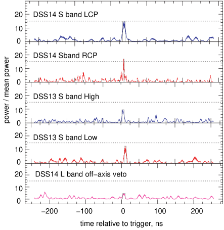
Figure 3: An example of a GLUE triggered event.

The field strength (V/m/MHz) from a cascade of total energy $W_{T}$ in regolith material can be expressed zhsa :

$$E=\frac{1.45\times 10^{-7}}{R}\ \frac{W_{T}}{1{\rm TeV}}\ \frac{\nu}{\nu_{0}}\ \frac{1}{(1+(\nu/\nu_{0})^{1.44})}$$ (1)

where $R$ is the distance to the source in meters, $\nu$ is the radio frequency, and the decoherence frequency is $\nu_{0}\simeq 2500$ MHz for the regolith ($\nu_{0}$ scales mainly by radiation length). For typical parameters in our experiment, a $10^{20}$ eV cascade will result in a peak field strength at Earth of $E\simeq 1.3~{}\mu$V m^-1 for a 70 MHz bandwidth. We have verified Equation 1 to within a factor of $2$ through accelerator tests Sal01 using silica sand targets and $\gamma$-ray-induced cascades with composite $W_{T}\sim 10^{19}$ eV.

Based on the effective antenna aperture $\eta A$ and the fact that the background events are due to fluctuations in the black-body power of the Moon, we estimate that the minimum detectable field strength for a linearly polarized pulse is

$$E_{min}~{}=~{}N_{\sigma}\sqrt{{2kT_{sys}Z_{0}\over\eta A\Delta\nu\sqrt{\epsilon}}},$$ (2)

where $Z_{0}=377\Omega$, and $N_{\sigma}$ the number of standard deviations required per channel relative to thermal fluctuations. For the lunar observations on the limb, which make up about 85% of the data reported here, $T_{sys}\simeq 110$ K (including the source contribution), $\nu=2.2$ GHz, and the average $\Delta\nu\simeq 70$ MHz. For the 70 m antenna, with $\eta\simeq 0.8$, the minimum detectable field strength at $N_{\sigma}=6$ is $E_{min}\simeq 0.8\mu$V m^-1. The estimated cascade threshold energy for these parameters is $W_{thr}=6\times 10^{19}$ eV. Since the mean inelasticity is $\langle y\rangle=0.2$, the threshold neutrino energy is $\sim 3\times 10^{20}$ eV.

Effective volume and acceptance vs. neutrino energy has been estimated via two independent Monte Carlo simulations, including the current estimates of both charged and neutral current cross sections Gan00 , and the $y$ distribution. The neutrino species are assumed to be fully mixed upon arrival. All neutrino flavors were included, and LPM effects in the shower formation were estimated zhsa . At each neutrino energy, a distribution of cascade angles and depths with respect to the local surface was obtained, and a refraction propagation of the predicted Cherenkov angular distribution was made through the regolith surface, including absorption, reflection, and roughness effects, and thermal noise fluctuations in the detector.

Via ray-tracing in our simulations (see Ref. Gor01 ), we find that, although the specific flux density of the events are lowered by a factor of order 2 from refraction and scattering, the effective volume and acceptance solid angle are increased by as much as an order of magnitude. The neutrino acceptance solid angle is thus about a factor of 20 larger than the apparent solid angle of the Moon itself. UHE cosmic rays could produce a background for lunar neutrino detection; however, there are several processes that suppress cosmic ray radio emission with respect to that of neutrinos, including total internal reflection, and formation zone effects Gor01 . The level of the potential UHE cosmic ray background is unknown, but as we have detected no events of any kind, our limits obtain in any case.

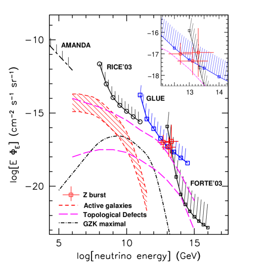
Figure 4: Model neutrino fluxes & limits from the present work and other current experiments. The inset expands the region near the Zburst predictions.

Figure 4 plots the predicted fluxes of ultra-high energy (UHE) neutrinos from AGN production Man96 ; Steck91 , a maximal flux from UHE cosmic-ray interactions Engel01 , two topological defect models Yos97 , and the Z-burst scenario Wei99 . Two other current limits in this energy regime are plotted, from the RICE experiment RICE03 , and the FORTE satellite FORTE03 . Our 90% confidence level, differential model-independent limit for 120 hours of livetime is shown plotted with large squares numbers , based on the observation of no events above an equivalent $6\sigma$ level amplitude (referenced to the 70 m antenna).

All of the differential limit curves in Fig. 4 (except for the $E_{\nu_{\mu}}^{-2}$ power law AMANDA limit) correspond to the inverse of the energy-dependent exposure = (neutrino aperture $\times$ time) Mlimits for each detector noted, scaled by the Poisson upper-limit factor (2.3 for 90% CL). Our plotted model-independent limit curves are very conservative, and become more restrictive when integrals over specific broad-spectrum models are considered. When converted to integral form, our limits constrain power-law neutrino models that parallel our curves for $\sim 1$ decade, even a factor of 3-5 below our plotted differential limits.

For quasi-monoenergetic models such as the Z-burst scenarios, the limits are exact, and the combined GLUE and FORTE results constrain much of the available Z-burst parameter space. Models such as the highest TD curve shown Yos97 are largely excluded at higher energies by the GLUE and FORTE results, since the integral (flux$~{}\times~{}$aperture) would lead to $\sim 3$ and $\sim 10$ events in each detector, respectively, in conflict with the null results.

We thank M. Klein, T. Kuiper, R. Milincic, and the Goldstone staff for their enthusiastic support. We are especially grateful to George Resch (d.2001) whose encouragement and unflagging support made this work possible. The work was performed in part at the Jet Propulsion Laboratory, California Institute of Technology, under contract with NASA, the Caltech President’s Fund, DOE contracts at Univ. of Hawaii and UCLA, the Sloan Foundation, and the National Science Foundation.

References

- (1) G. A. Askaryan, 1962, JETP 14, 441; 1965, JETP 21, 658.
- (2) D. Saltzberg, P. Gorham, D. Walz, et al. Phys. Rev. Lett., 86, 2802 (2001); P. W. Gorham, D. P. Saltzberg, P. Schoessow, et al., Phys. Rev. E. 62, 8590 (2000).
- (3) T. Weiler, 1999, hep-ph/9910316; and Z. Fodor, S. D. Katz, & A. Ringwald, Phys. Rev. Lett. 88 (2002), 171101; hep-ph/0105064.
- (4) S. Yoshida, H. Dai, C. C. H. Jui, & P. Sommers, 1997, Ap.J. 479, 547.Bhattacharjee, P., Hill, C.T., & Schramm, D.N, 1992 Phys.Rev.Lett 69, 567.
- (5) T. Weiler, Phys. Rev. Lett. (1982), 49, 234.
- (6) I. M. Zheleznykh, 1988, Proc. Neutrino ’88, 528.
- (7) R. D. Dagkesamanskii, & I. M. Zheleznyk, 1989, JETP 50, 233.
- (8) T. H. Hankins, R. D. Ekers & J. D. O’Sullivan, 1996, MNRAS 283, 1027.
- (9) E. Zas, F. Halzen, & T. Stanev, 1992, Phys. Rev. D 45, 362; J. Alvarez–Muñiz, & E. Zas, 1997, Phys. Lett. B, 411, 218; J. Alvarez–Muñiz, & E. Zas, 2000, in Proc. of RADHEP 2000, AIP#579 (2001).
- (10) P. Gorham, et al., Proc. 26th ICRC, HE 6.3.15, astro-ph/9906504.
- (11) D. Morrison & T. Own, 1987 The Planetary System, (Addison-Wesley: Reading,MA).
- (12) G. R. Olhoeft & D. W. Strangway, 1975, Earth Plan. Sci. Lett. 24, 394.
- (13) R. Gandhi, Nucl.Phys.Proc.Suppl. 91 (2000) 453.
- (14) N. S. Soboleva, Soviet astronomy - AJ, 6(6), 873, (1963).
- (15) C. E. Heiles and F. D. Drake, Icarus 2, 281 (1963).
- (16) P. Gorham et al., in Proc. of RADHEP 2000, AIP#579 (2001), astro-ph/0102435.
- (17) Mannheim, K., 1996, Astropart. Phys 3, 295.
- (18) F.W. Stecker, et al., Phys. Rev. Lett. 66, 2697; E69, 2738 (1991); see also Stecker & Salamon, Space Sci. Rev. 75, 341 (1996)
- (19) R. Engel, et al., Phys.Rev.D 64, 093010, (2001).
- (20) L. A. Anchordoqui et al., Phys. Rev. D 66, 103002 (2002).
- (21) I. Kravchenko et al., for the RICE collaboration, submitted to Astroparticle Physics; astro-ph/0206371, (2003).
- (22) N. Lehtinen, P. Gorham, A. Jacobson, & R. Roussel-Duṕre, Phys.Rev.D 69 (2004) 013008; astro-ph/030965.
- (23) The values of the 8 plotted points are: -13.8,-15.4,-16.1,-16.7,-17.3,-17.7,-18.1,-18.4.
- (24) Similar to approaches described in ref. Anch02 and ref. FORTE03 , as well as earlier GLUE results Gor01 ; Gor99 .