Force-Free Magnetosphere of an Accretion Disk — Black Hole System. I. Schwarzschild Geometry

Abstract

In this paper I study the magnetosphere of a black hole that is connected by the magnetic field to a thin conducting Keplerian disk. I consider the case of a Schwarzschild black hole only, leaving the more interesting but difficult case of a Kerr black hole to a future study. I assume that the magnetosphere is ideal, stationary, axisymmetric, and force-free. I pay a special attention to the two singular surfaces present in the system, i.e., the event horizon and the inner light cylinder; I use the regularity condition at the light cylinder to determine the poloidal electric current as a function of poloidal magnetic flux. I solve numerically the Grad–Shafranov equation, which governs the structure of the magnetosphere, for two cases: the case of a nonrotating disk and the case of a Keplerian disk. I find that, in both cases, the poloidal flux function on the horizon matches a simple analytical expression corresponding to a radial magnetic field that is uniform on the horizon. Using this result, I express the poloidal current as an explicit function of the flux and find a perfect agreement between this analytical expression and my numerical results.

1 Introduction

It has been broadly acknowledged that magnetic fields around accreting black holes are very important. Magnetic interaction between a spinning black hole and remote astrophysical loads is often invoked to explain many observed features of Active Galactic Nuclei (AGNs) and Galactic black holes (e.g., Begelman, Blandford, & Rees 1984; Krolik 1999; Punsly 2001). In particular, magnetic configurations in which the field lines threading a black hole extend to infinity have been studied very extensively and have gained a lot of popularity as the standard model for jet production. In this model, the black hole’s rotational energy is extracted electromagnetically by the means of the famous Blandford–Znajek mechanism (Blandford & Znajek 1977, hereafter BZ77; Macdonald & Thorne 1982, hereafter MT82; Phinney 1983; Macdonald 1984; Thorne et al. 1986; Komissarov 2001) and is transported outward in the form of Poynting flux to power a jet.

Recently, however, another magnetic configuration has become a subject of growing interest — a configuration where at least some part of magnetic field lines connect the black hole and the accretion disk (e.g., MT82; Nitta et al. 1991; Hirotani et al. 1992; Blandford 1999, 2000; Gruzinov 1999; Li 2000, 2001, 2002; Wang et al. 2002, 2003). In this so-called Magnetically-Coupled (MC) configuration (Wang et al. 2002) the magnetic field couples the hole directly to the disk and transfers angular momentum between the two; it can thus regulate the spin evolution of the black hole (Wang et al. 2002, 2003). In addition, the magnetic link provides a means to extract the rotational energy of the black hole (in a manner similar to the BZ77 mechanism) and to transport it to the inner region of the disk. This effect may lead to some additional heating and an increase in the luminosity of the inner part of the disk, with important observational implications (Gammie 1999; Li 2000, 2001, 2002). Another reason for interest in the MC configuration is the suggestion that twisted (due to a mismatch of rotation rates of the hole and the disk) field lines may become unstable, leading to strong variability on the rotation time scale and possibly to Quasi-Periodic Oscillations (QPOs), as suggested by Gruzinov (1999). QPOs may also be produced by non-axisymmetries of the magnetic field connecting the hole to the disk and the associated non-axisymmetry of local disk heating (Li 2001, 2002).

In theoretical studies of both the BZ77 and MC processes, researchers (including Blandford & Znajek themselves) have often employed the framework of force-free electrodynamics. Within this framework, the plasma in the magnetosphere above the accretion disk is assumed to have such a low density that it is completely unimportant dynamically. At the same time, the plasma is dense enough to carry the necessary currents and charges without significant dissipation. This framework has proven to be very useful as it apparently provides the minimal nontrivial level of description required by the magnetospheric conditions. Under the usual additional assumptions of time stationarity and axisymmetry, the main fundamental mathematical formulation of this framework is the so-called Grad–Shafranov equation. Over the years, there have been a number of attempts to solve this rather nontrivial nonlinear Partial Differential Equation (PDE) in the context of a black-hole magnetosphere with open magnetic field. These studies include both semi-analytical models that use some sort of a self-similar ansatz (e.g., BZ77), and also the most general numerical computations (e.g., Macdonald 1984; Fendt 1997; Komissarov 2001). At the same time, however, there have been, to the best of my knowledge, no numerical or analytical attempts to solve the Grad–Shafranov equation in the context of the magnetically-linked black hole–disk system.

The goal of this paper is to remedy this situation by providing the first numerical solution of the Grad–Shafranov equation for the MC configuration. In order to achieve this goal, one first needs to examine the structure of the equation and, in particular, understand the role of, and devise a proper mathematical treatment for, the singular surfaces of the Grad–Shafranov equation, namely the Event Horizon and the Light Cylinder. One very important thing I would like to emphasize in this regard is that the condition of regularity at the light cylinder is crucial; indeed, it is this conditions that enables one to fix the poloidal current function and hence the toroidal magnetic field. This point of view is very close in spirit to that of Beskin & Kuznetsova (2000), who suggested a similar approach for the full-MHD case. I also would like to add that, in this respect, the situation is very similar to the problem of axisymmetric pulsar magnetosphere, where the light-cylinder regularity condition plays a similar role (Contopoulos et al. 1999; Uzdensky 2003). As for the event horizon, it plays only a passive role here, similar to that of the asymptotic infinity (see, e.g., Punsly 1989; Punsly & Coroniti 1990). Thus, the horizon is, in a sense, less important; for example, one cannot set any boundary conditions on it (e.g., Beskin 1997; Beskin & Kuznetsova 2000).

Although the most interesting and general case is that of a rapidly-rotating Kerr black hole, in the present work I restrict myself to the simpler case of a nonrotating, Schwarzschild black hole. This work should thus be viewed as a first starting step. Even the Schwarzschild case, however, is not entirely trivial, because the disk and, hence, the magnetosphere are still (nonuniformly!) rotating, and thus the Grad–Shafranov equation is still nonlinear and has singular surfaces.

Considering the Schwarzschild case first has a purely technical advantage of having to deal with fewer terms in the equations. In addition, a closed-field solution is certain to exist in this case; whether it exists in the more general Kerr case is not so clear. Indeed, it may be that, for a sufficiently rapidly-rotating hole, a completely closed (i.e., with all the field lines threading both the event horizon and the disk) configuration may not be possible, that is, some fraction of the field lines may have to be open and to extend from the hole to infinity. This scenario could be characterized as a hybrid between the BZ77 and MC configurations, as suggested by Wang et al. (2002, 2003). I plan to consider such a configuration in full Kerr geometry in the near future.

Finally, I would like to remark that a black hole–disk MC configuration differs greatly from the case where the central object is a star with a highly-conducting surface, such as a neutron star or a young star. In that latter case, the differential rotation between the disk and the conducting star inevitably leads to the inflation and opening of the field lines on the rotation time scale. This, in turn, makes a steady state impossible (e.g., van Ballegooijen 1994; Lovelace et al. 1995; Uzdensky et al. 2002). In contrast, in the case of a black hole being the central object, a steady configuration is, in principle, possible (at least in the Schwarzschild case). This is because the rather large “effective resistivity” of the event horizon (in the Membrane-Paradigm description; see Znajek 1977, 1978; Damour 1978; Thorne et al. 1986) makes it possible for the field lines rotating with the disk’s angular velocity to slip through the horizon. This important fact makes the study of a black hole’s magnetosphere conceptually simpler than that of a regular star, even though the proper treatment of the black-hole case is unavoidably plagued with technical difficulties, such as having to work in curved space-time.

In § 2 I outline the basic equations that describe a stationary axisymmetric force-free magnetosphere in Schwarzschild geometry; in particular, I discuss the Grad–Shafranov Equation. In the same section I also describe the boundary conditions pertinent to the MC configuration under consideration. In § 3 I discuss the singular surfaces of the Grad–Shafranov equation and the regularity conditions set on these surfaces. In particular, § 3.1 is devoted to the regularity condition at the event horizon and § 3.2 is devoted to the light-cylinder regularity condition. Next, in § 4, I consider a particularly simple but very important case of a nonrotating disk around a nonrotating black hole. In this case the light cylinder merges with the horizon and the Grad–Shafranov becomes linear. I solve this equation numerically and find that the radial magnetic field is uniform on the event horizon. In § 5 I consider the limit of a slowly-rotating disk and derive explicit analytical expressions for the location and the shape of the light cylinder and for the poloidal current. I illustrate these ideas by considering one particular manifestation of the slow-rotation limit, namely, a Keplerian disk. I present my numerical solution of the full, nonlinear Grad–Shafranov equation for this case and find a perfect agreement between the numerical results and the above-mentioned analytical predictions. Finally, in § 6 I present my conclusions and discuss possible extensions of my present work and the directions for future research.

2 Stationary Axisymmetric Force-Free Magnetosphere in Schwarzschild Geometry

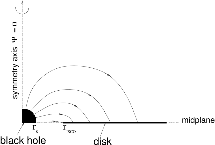
Figure 1: Schematic drawing of an axisymmetric linked Black Hole – Disk magnetosphere.

I consider a steady-state force-free magnetosphere of a Schwarzschild Black Hole surrounded by a thin, rotating, infinitely-conducting accretion disk. I am interested only in the large-scale magnetic field, ignoring any small-scale and intermittent field structures. I assume the topology of this global magnetic field to be such that all the field lines connect the disk to the event horizon (or, rather, the stretched horizon of the Membrane Paradigm, see Thorne et al. 1986) of the black hole (see Fig. 1); in particular this means that there are no open field lines extending out to infinity. I also assume that the system possesses axial symmetry and reflection symmetry with respect to the equatorial disk plane.

Magnetic field lines are assumed to be frozen into the disk. Also, whereas inside the disk the magnetic field is considered to be dynamically unimportant, in the very tenuous magnetosphere above the disk the electromagnetic forces are assumed to be dominant over the inertial, gravitational, and pressure forces. Under these conditions, the structure of the magnetosphere is governed by the force-free equation:

$$\rho_{e}{\bf E}\,+{{\bf j\times B}\over c}=0\,,$$ (1)

where all the electromagnetic quantities are measured by the Fiducial Observers (FIDOs), see MT82 and Thorne et al. (1986).

At this point, however, I have to make the following remark. In a realistic situation the force-free approximation is bound to break down close enough to the event horizon, as the plasma inertia and gravity necessarily start to dominate the dynamics there. In particular, the black hole is always enveloped by a fast magnetosonic critical surface. Nevertheless, as the plasma density is taken to zero, this fast critical surface moves in infinitesimally close to the horizon (e.g., Beskin 1997). This fact makes it possible to effectively extend the domain of validity of the force-free approximation all the way to the horizon. At the same time, however, this “full-MHD origin” of the force-free equation is important, because it provides one with an additional condition that leads to a way to regularize the force-free solution at the event horizon (see § 3.1). Such a regularization is possible because the solutions of the full-MHD set of equations are automatically free of certain singularities that are admitted, in principle, by the force-free equation.

The geometry of space-time around a Schwarzschild Black hole is described by

$$ds^{2}=-\alpha^{2}dt^{2}+\alpha^{-2}dr^{2}+r^{2}d\theta^{2}+r^{2}\sin^{2}\theta\,d\phi^{2}\,,$$ (2)

where

$$\alpha(r)\equiv\sqrt{1-{r_{s}\over r}}$$ (3)

is the lapse function and $r_{s}\equiv 2GM/c^{2}$ is the Schwarzschild radius of the event horizon.

I employ the 3+1 split of laws of electrodynamics, introduced by MT82. In this approach, Maxwell’s equations in Schwarzschild geometry take the following form:

$$\nabla\cdot{\bf E}=4\pi\rho_{e}\,,$$ (4)

$$\nabla\cdot{\bf B}=0\,,$$ (5)

$$\nabla\times(\alpha{\bf E})=-{1\over c}\,\partial_{t}{\bf B}\,,$$ (6)

$$\nabla\times(\alpha{\bf B})={1\over c}\,\partial_{t}{\bf E}+{{4\pi\alpha}\over c}\,{\bf j}\,.$$ (7)

An axisymmetric magnetic field can be written in terms of two functions $\Psi(r,\theta)$ and $I(r,\theta)$ as

$${\bf B(r,\theta)}={\bf B}_{\rm pol}+{\bf B}_{\rm tor}=\nabla\Psi\times\nabla\phi+{I\over{\alpha}}\,\nabla\phi\,,$$ (8)

where $\Psi$ is the poloidal magnetic flux function and $I$ is $(2/c)$ times the poloidal electric current flowing through the circular loop $r={\rm const}$, $\theta={\rm const}$. Note that the choice of sign in this definition of $I$ is consistent with the choice made by Mobarry & Lovelace (1986) but is opposite to that by MT82.

I use the orthonormal basis $\{{\bf e}_{\hat{\alpha}}\}=\{{\bf e}_{\hat{r}},{\bf e}_{\hat{\theta}},{\bf e}_{\hat{\phi}}\}$, where ${\bf e}_{\hat{\alpha}}=g_{\alpha\alpha}^{-1/2}\partial_{\alpha}$ (note: there is no summation over $\alpha$ in this expression), that is

$${\bf e}_{\hat{r}}=\alpha\,\partial_{r},\quad{\bf e}_{\hat{\theta}}={1\over r}\,\partial_{\theta},\quad{\bf e}_{\hat{\phi}}={1\over{r\sin\theta}}\,\partial_{\phi}\,.$$ (9)

In Schwarzschild metric (2), the 3-gradient of an arbitrary function $\chi(r,\theta,\phi)$ is calculated as follows:

$$\nabla\chi=\alpha\,(\partial_{r}\chi)\,{\bf e}_{\hat{r}}+{1\over r}\,(\partial_{\theta}\chi)\,{\bf e}_{\hat{\theta}}+{1\over{r\sin\theta}}\,(\partial_{\phi}\chi)\,{\bf e}_{\hat{\phi}}\,.$$ (10)

Thus,

$$\nabla\Psi(r,\theta)=\alpha\,(\partial_{r}\Psi)\,{\bf e}_{\hat{r}}+{1\over r}\,(\partial_{\theta}\Psi)\,{\bf e}_{\hat{\theta}}\,,$$ (11)

and

$$\nabla\phi={1\over{r\sin\theta}}\,{\bf e}_{\hat{\phi}}\,.$$ (12)

Applying this to expression (8) for the magnetic field components, one gets

$${\bf B}_{\rm pol}=\nabla\Psi\times\nabla\phi={1\over{r\sin\theta}}\,{{\partial\Psi}\over{r\partial\theta}}\,{\bf e}_{\hat{r}}-{\alpha\over{r\sin\theta}}\,{{\partial\Psi}\over{\partial r}}\,{\bf e}_{\hat{\theta}}\,,$$ (13)

and

$${\bf B_{\rm tor}}={I\over\alpha}\nabla\phi={I\over{\alpha r\sin\theta}}\,{\bf e}_{\hat{\phi}}\,.$$ (14)

As for the electric field, it can be shown that, under the conditions of axisymmetry, stationarity, and ideal magnetohydrodynamics (MHD), i.e., ${\bf E\cdot B}=0$, it is given by

$$E_{\hat{\phi}} = 0\,,$$ (15)

$${\bf E}_{\rm pol} = -\,{1\over{\alpha c}}\ \Omega(\Psi)\,\nabla\Psi\,,$$ (16)

where $\Omega(\Psi)$ is the angular velocity of the field lines.

As I have mentioned earlier, the main equation determining the structure of the magnetosphere is the force-free equation (1). Upon examining the toroidal component of this equation, one immediately sees that poloidal current $I$ has to be constant along magnetic field lines:

$$I=I(\Psi)\,.$$ (17)

Thus, the electromagnetic field in a stationary axisymmetric ideal-MHD force-free magnetosphere is completely described by the poloidal magnetic flux function $\Psi(r,\theta)$ and two functions of $\Psi$, namely, $\Omega(\Psi)$ and $I(\Psi)$.

Next, one can show that the two poloidal components of the force-free equation (1) can be combined into the force-free Grad–Shafranov equation for the poloidal flux function $\Psi(r,\theta)$. In the most general Kerr-metric case this equation has first been derived in the full four-dimensional framework by BZ77 and then later by MT82, who had used the language of the 3+1 split (see also Beskin 1997). Subsequently, it has been generalized to full general-relativistic MHD including the effects of plasma inertia and pressure (e.g., Nitta et al. 1991; Beskin & Par’ev 1993). In the specific case of Schwarzschild geometry, the full-MHD Grad–Shafranov equation, along with its simpler, force-free version, has been derived and discussed by Mobarry & Lovelace (1986). Here I shall use their force-free Grad–Shafranov equation (44); in my notation it can be written as follows (I set the speed of light $c$ and the gravitational constant $G$ both equal to one throughout this paper):

$$(\alpha^{2}-R^{2}\Omega^{2})\,\Delta^{*}\Psi={\alpha^{4}\over{2R^{2}}}\,\nabla\Psi\cdot\nabla\biggl{(}{{R^{4}\Omega^{2}}\over\alpha^{4}}\biggr{)}-II^{\prime}(\Psi)\,,$$ (18)

where

$$R\equiv r\sin\theta\,,$$ (19)

and

$$\Delta^{*}\Psi\equiv\partial_{r}(\alpha^{2}\partial_{r}\Psi)+{\sin\theta\over r^{2}}\,\partial_{\theta}\,\biggl{(}{1\over{\sin\theta}}\,\partial_{\theta}\Psi\biggr{)}$$ (20)

is the linear Grad–Shafranov operator in Schwarzschild geometry.

Equation (18) is a nonlinear second-order elliptic PDE for the function $\Psi(r,\theta)$; the right-hand side (RHS) of this equation contains no second-order derivatives of $\Psi$, but does contain terms that are linear and quadratic in the first order derivatives of $\Psi(r,\theta)$. One can rewrite this equation in the following alternative form, more suitable for further calculations:

$$(\alpha^{2}-R^{2}\Omega^{2})\,\biggl{(}\alpha^{2}\partial_{r}^{2}\Psi+{1\over r^{2}}\,\Delta_{\theta}^{*}\Psi\biggr{)} + \alpha^{2}[\alpha^{2}(r)]^{\prime}\,\partial_{r}\Psi=$$

$$\Omega\Omega^{\prime}(\Psi)\,R^{2}|\nabla\Psi|^{2}\, - II^{\prime}(\Psi)+\Omega^{2}\biggl{(}2\alpha^{2}\sin^{2}\theta\,r\,\partial_{r}\Psi+\sin{2\theta}\,\partial_{\theta}\Psi\biggl{)}\,,$$ (21)

where

$$\Delta_{\theta}^{*}\Psi\equiv\sin\theta\,{\partial\over{\partial\theta}}\,\biggl{(}{1\over{\sin\theta}}\,{\partial\Psi\over{\partial\theta}}\biggr{)}$$ (22)

is the poloidal-angle part of the Grad–Shafranov operator and

$$|\nabla\Psi|^{2}=\alpha^{2}\biggl{(}{{\partial\Psi}\over{\partial r}}\biggr{)}^{2}+{1\over{r^{2}}}\,\biggl{(}{{\partial\Psi}\over{\partial\theta}}\biggr{)}^{2}\,.$$ (23)

In flat space with Euclidean geometry, $\alpha=1={\rm const}$, equation (21) becomes

$$(1-R^{2}\Omega^{2})\,\biggl{(}\partial_{r}^{2}\Psi+{1\over r^{2}}\,\partial_{\theta}^{2}\Psi\biggr{)} - (1+R^{2}\Omega^{2})\,{{\cot\theta}\over{r^{2}}}\,\partial_{\theta}\Psi-2\Omega^{2}\,r\sin^{2}\theta\,\partial_{r}\Psi$$ (24)

$$= \Omega\Omega^{\prime}(\Psi)\,R^{2}\,|\nabla\Psi|^{2}-II^{\prime}(\Psi)\,,$$

which can be immediately recognized as the familiar pulsar equation with $\Omega=\Omega(\Psi)\neq{\rm const}$ (e.g., Okamoto 1974).

In Schwarzschild geometry, the radial derivative of the square of the lapse function $\alpha$ is $[\alpha^{2}(r)]^{\prime}=r_{s}/r^{2}$, and so one can rewrite (21) in the following final form:

$$(\alpha^{2}-R^{2}\Omega^{2})\,\biggl{(}\alpha^{2}\partial_{r}^{2}\Psi+{1\over r^{2}}\,\partial_{\theta}^{2}\Psi\biggr{)} - (\alpha^{2}+R^{2}\Omega^{2})\,{{\cot\theta}\over{r^{2}}}\,\partial_{\theta}\Psi+{\alpha^{2}\over r}\,\biggl{(}{r_{s}\over r}-2R^{2}\Omega^{2}\biggr{)}\,\partial_{r}\Psi$$ (25)

$$= \Omega\Omega^{\prime}(\Psi)\,R^{2}\,|\nabla\Psi|^{2}-II^{\prime}(\Psi)\,.$$

Let us now discuss the boundary conditions that supplement equation (18) [or its equivalent forms (21) and (25)]. First, the rotation axis is a field line, so let us set

$$\Psi(r,\theta=0)=0\,.$$ (26)

Second, since we are considering the case where all the field lines are closed, i.e., go from the black hole to the disk, the flux function has to vanish at infinity:

$$\Psi(r=\infty,\theta)=0\,.$$ (27)

Third, we consider a disk that does not extend all the way to the event horizon but instead ends abruptly at a certain inner-edge radius $r_{\rm in}$. The most natural choice for $r_{\rm in}$ is $r_{\rm ISCO}$, the radius the Innermost Stable Circular Orbit (ISCO) (equal to $6M$ for a Schwarzschild black hole); at this point in the discussion, however, one can just leave $r_{\rm in}>r_{s}$ unspecified. I assume that the magnetic field lines are frozen into the disk beyond $r_{\rm in}$, with some given (but, at this point, arbitrary) magnetic flux distribution:

$$\Psi(r\geq r_{\rm in},\theta=\pi/2)=\Psi_{d}(r)\,.$$ (28)

The region $(r_{s}\leq r\leq r_{\rm in},\theta=\pi/2)$ that separates the disk from the black hole is generally referred to as the plunging region. Here the infalling matter can no longer be supported against gravity by the centrifugal force; hence, it presumably falls very rapidly towards the black hole. As a result, magnetic loops are strongly stretched in the radial and azimuthal directions and the vertical magnetic field is greatly diminished. Under these circumstances, it is natural to choose the plunging-region boundary condition in the following form:

$$\Psi(r_{s}\leq r\leq r_{\rm in},\theta=\pi/2)=\Psi_{\rm max}\equiv\Psi_{d}(r_{\rm in})={\rm const}\,.$$ (29)

Finally, one cannot and, indeed, need not specify any boundary conditions at the event horizon. This is because the horizon, being an analog of spatial infinity, cannot emit waves that carry information outward and is thus casually disconnected from the outside magnetosphere (e.g., Punsly 1989; Punsly & Coroniti 1990). Within the force-free framework, the mathematical basis for this statement lies in the fact that the horizon is a singular surface of the Grad–Shafranov equation. Therefore, one can only apply some regularity conditions there (see § 3.1 for a detailed discussion).

Notice that specifying the boundary conditions is not enough for a complete problem set-up. Indeed, the force-free Grad–Shafranov equation (18) [and its equivalent forms (21) and (25)] also involves two, a priori unknown, functions of $\Psi$, i.e., $\Omega(\Psi)$ and $I(\Psi)$; therefore, one also needs to discuss what determines these two functions. First, in the problem considered in this paper, it is in fact very easy to find $\Omega(\Psi)$. Indeed, since the field lines are assumed to be frozen into the disk, each field line has to rotate with the angular velocity of its footpoint on the disk surface:

$$\Omega(\Psi)=\Omega_{d}[r_{0}(\Psi)]\,.$$ (30)

Here, $\Omega_{d}(r)$ is a prescribed disk rotation law (e.g., Keplerian) and $r_{0}(\Psi)$ is the radial position of the footpoint of field line $\Psi$ on the surface of the disk; it is related to the function $\Psi_{d}(r)$ via $\Psi_{d}[r_{0}(\Psi)]=\Psi$.

As for the other function, i.e., $I(\Psi)$, it is not physically appropriate to try to specify it explicitly at the surface of the disk or at the event horizon. The basic reason for this is the following. The Grad–Shafranov equation is a second-order PDE with two singular surfaces and two unknown functions of $\Psi$ (i.e., two “integrals of motion”), $\Omega(\Psi)$ and $I(\Psi)$. Hence, one can (and indeed needs to) specify only two functions at the boundaries (see Beskin 1997) and I have already chosen both of these functions, $\Psi_{d}(r)$ and $\Omega(\Psi)=\Omega_{K}[r_{0}(\Psi)]$, to be specified on the disk surface [see eqs. (28) and (30)]. Therefore, trying to specify directly one more function, such as $I(\Psi)$, would over-constrain the system. Instead, as I discuss in detail in § 3.2, the correct way to determine $I(\Psi)$ is through the use of the regularity condition at the inner light cylinder.

3 Regularity Conditions on the Singular Surfaces of the Grad–Shafranov Equation (for $\Omega\neq 0$)

As one can easily see from the Grad–Shafranov equation in the form (25), a force-free magnetosphere of a Schwarzschild black hole (with the closed-field configuration considered here) has two regular singular surfaces on which the coefficients in front of the highest order derivatives of $\Psi$ vanish. These are the Event Horizon $\alpha=0$ (or $r=r_{s}=2M$) and the Light Cylinder $\alpha^{2}=R^{2}\Omega^{2}$. On each of these two surfaces I am going to impose a corresponding regularity condition; these two regularity conditions are going to be indispensable in my analysis.

The first of the two surfaces, i.e., the event horizon, is singular because the coefficient $\alpha^{2}\equiv 1-r_{s}/r$ in front of the second-order radial (i.e., normal to this surface) derivative becomes zero. This surface is the limit of the fast magnetosonic surface as the plasma density goes to zero. Correspondingly, as one analyses the low-density limit of the full-MHD Grad–Shafranov equation, one finds that the critical condition on the fast surface turns into the event-horizon regularity condition (Beskin 1997). Since one of the boundaries of the domain coincides with the event horizon, I shall use the regularity condition at the horizon in lieu of a boundary condition for $\Psi(r,\theta)$ at $r=r_{s}$ (see § 3.1).

The second singular surface, namely, the light cylinder, can be characterized as the surface where the magnitude of the electric field is equal to that of the poloidal magnetic field, and, correspondingly, where the toroidal velocity of the rotating field lines, $v_{\bf B}=R\Omega/\alpha$ equals the speed of light. I shall use the regularity condition at the light cylinder as the main condition that fixes the function $I(\Psi)$ (see § 3.2).

It is important to note that, in contrast to a rigidly-rotating pulsar magnetosphere, in the case of an accreting black hole, where the field lines are tied to a differentially-rotating Keplerian disk, the angular velocity $\Omega$ is a (non-constant) function of $\Psi$. Hence, the spatial location and even the shape of the light cylinder are not known a priori; they need to be determined self-consistently as a part of the whole solution. Also note that the light cylinder, that one has to deal with in the problem considered here, is the so-called inner light cylinder. In a more general situation, where some of the field lines are open and extend to infinity, there may be two light cylinders: the outer one and the inner one (Znajek 1977; BZ77). The outer light cylinder is crossed at large distances by the open field lines and is a direct analog of the light cylinder in pulsar magnetospheres. The inner light cylinder is crossed much closer to the black hole by the field lines threading the event horizon; its existence is a purely general-relativistic (GR) effect; it is due to the fact that the expression for the electric field (16) has the additional factor $1/\alpha$ as compared with the non-GR expression.

3.1 Regularity Condition at the Event Horizon

Let us now discuss the behavior of the flux function in the vicinity of the event horizon. In general, equation (25) admits solutions that are not regular at the horizon. In particular, the two indicial exponents of the linear part of equation (25) are equal to zero and one; hence, one can expect the asymptotic expansion near $r=r_{s}$ to contain logarithmic terms in addition to pure power laws (e.g., Bender & Orszag 1978). Taking into account that the magnetic flux must be finite on the horizon (see below), one can write the first few terms in the asymptotic expansion of a general solution of the full nonlinear equation (25) as

$$\Psi(r\rightarrow r_{s},\theta) = \Psi_{0}(\theta)+\tilde{\Psi}_{1}(\theta)(r-r_{s})\log(r-r_{s})+\Psi_{1}(\theta)(r-r_{s})$$ (31)

$$+ \hat{\Psi}_{2}(\theta)(r-r_{s})^{2}\log^{2}(r-r_{s})+\tilde{\Psi}_{2}(\theta)(r-r_{s})^{2}\log(r-r_{s})$$

$$+ \Psi_{2}(\theta)(r-r_{s})^{2}\ +\ ...$$

Here, the presence of the $(r-r_{s})^{2}\log^{2}(r-r_{s})$-term is due to the nonlinear term $R^{2}\,\Omega\Omega^{\prime}|\nabla\Psi|^{2}$ that appears on the RHS of the Grad–Shafranov equation.

A physically-reasonable solution, however, should be free of the logarithmic terms, as we shall see below. One can trace the origin of this regularity requirement to the full-MHD framework’s condition of regularity at the fast magnetosonic surface, as one makes the transition to the force-free limit (e.g., Beskin 1997; Beskin & Kuznetsova 2000). The physical meaning of the event-horizon regularity condition has been discussed beautifully by MT82 and by Thorne et al. (1986). My discussion here follows their line of thought.

According to MT82 and Thorne et al. (1986), the only condition that one can impose at the event horizon is the requirement that the physically-reasonable Freely-Falling Observer (FFO) measures finite fields ${\bf E}_{FFO}$ and ${\bf B}_{FFO}$ near the horizon. In order to determine the behavior of the fields measured by the FIDO, one then has to perform a Lorentz transformation from the FFO frame to the FIDO frame. This transformation is a radial boost with the velocity $v=2M/r$, which corresponds to $\gamma=1/\alpha$. The result is:

$${\bf E}_{\perp},\ {\bf B}_{\perp}\qquad-\quad{\rm finite;}$$ (32)

$${\bf E}_{\parallel},\ {\bf B}_{\parallel}\propto{1\over\alpha},\quad\alpha\rightarrow 0\,;$$ (33)

but

$${\bf E}_{\parallel}-{\bf n}\times{\bf B}_{\parallel}\sim\alpha,\quad\alpha\rightarrow 0\,.$$ (34)

(Here the $\perp$ sign describes the perpendicular to the event horizon, i.e., radial, component, and the $\parallel$ sign describes the parallel to the event horizon, i.e., the $\phi$ and $\theta$, components.)

First, from equation (32) it follows that $\Psi(r_{s},\theta)$ must be finite, as we have already anticipated.

Next, consider equation (34); it has two components ($\phi$ and $\theta$) and I shall consider them separately. First, since $E_{\hat{\phi}}=0$ according to equation (15), the $\phi$-component of equation (34) gives

$$B_{\hat{\theta}}=O(\alpha)\qquad\Rightarrow\qquad{\partial\Psi\over{\partial r}}=\ {\rm finite\ at}\quad\alpha=0\,.$$ (35)

Thus, $\tilde{\Psi}_{1}(\theta)\equiv 0$ and the expansion (31) near the horizon becomes:

$$\Psi(r,\theta) = \Psi_{0}(\theta)+\Psi_{1}(\theta)(r-r_{s})+\hat{\Psi}_{2}(\theta)(r-r_{s})^{2}\log^{2}(r-r_{s})$$ (36)

$$+ \tilde{\Psi}_{2}(\theta)(r-r_{s})^{2}\log(r-r_{s})\ +\ \Psi_{2}(\theta)(r-r_{s})^{2}\ +\ ...$$

The condition (35) may seem trivial, but notice that everywhere in equation (25) the first- and second-order radial derivatives of $\Psi$ appear only in a combination with $\alpha$ or $\alpha^{2}$. Thus, without condition (35), it would in principle be possible for these derivatives to diverge in the limit $r\rightarrow r_{s}$, while leaving the product $\alpha^{2}\partial_{r}^{2}\Psi$ finite and comparable with all the other (regular) terms near the event horizon. It is only due to condition (35) that one can discard all such solutions and hence drop all the terms proportional to $\alpha$ when applying equation (25) at the horizon. One then gets the following equation:

$$II^{\prime}(\Psi_{0})=\Omega(\Psi_{0})\sin\theta\biggl{[}\Omega^{\prime}\sin\theta\biggl{(}{{d\Psi_{0}}\over{d\theta}}\biggr{)}^{2}+\Omega\cos\theta{{d\Psi_{0}}\over{d\theta}}+\Omega\sin\theta{{d^{2}\Psi_{0}}\over{d\theta^{2}}}\biggr{]}\,.$$ (37)

In other words, equation (37) is obtained by substituting expansion (36) into the Grad–Shafranov equation (25) and looking at the terms of lowest order in $(r-r_{s})$. Furthermore, when one looks at the balance in the next two orders in $(r-r_{s})$, namely $O[(r-r_{s})\log^{2}(r-r_{s})]$ and $O[(r-r_{s})\log(r-r_{s})]$, one can deduce that $\hat{\Psi}_{2}(\theta)=0=\tilde{\Psi}_{2}(\theta)$, and so $\partial_{r}^{2}\Psi$ must be finite at the event horizon.

It is interesting to note that not only the second, but also the first radial derivatives of $\Psi$ drop out of the Grad–Shafranov equation when $\alpha$ is set to zero. One thus sees that, upon using the regularity condition (34), the Grad–Shafranov differential equation becomes an algebraic equation at the event horizon, as far as the radial direction is concerned; it is of course still a differential equation in the $\theta$-direction. The resulting equation (37) can be viewed as an Ordinary Differential Equation (ODE) that determines the function $\Psi_{0}(\theta)\equiv\Psi(r=r_{s},\theta)$, provided that both $I(\Psi)$ and $\Omega(\Psi)$ are known.

Equation (37) can be readily integrated, resulting in

$$I(\Psi_{0})=\pm\Omega(\Psi_{0})\sin\theta\,{{d\Psi_{0}}\over{d\theta}}\,,$$ (38)

where I set the integration constant equal to zero because I require the poloidal current $I(\Psi)$ to vanish at the pole $\theta=0$. One can integrate (38) further to determine (albeit implicitly) the function $\Psi_{0}(\theta)$:

$$\int\limits_{0}^{\Psi_{0}}{{\Omega(\Psi_{0})}\over{\pm I(\Psi_{0})}}d\Psi_{0}=\int\limits_{0}^{\theta}{d\theta\over{\sin\theta}}\,,$$ (39)

where I have used the boundary condition $\Psi_{0}(\theta=0)=0$.

Notice that, in principle, the regularity condition (38), derived from the $\phi$ component of equation (34), admits both plus and minus signs. In order to break this degeneracy, one needs to use the remaining condition, namely the $\theta$ component of equation (34):

$$E_{\hat{\theta}}+B_{\hat{\phi}}=O(\alpha),\qquad\alpha\rightarrow 0\,.$$ (40)

According to equations (14) and (16), both $B_{\hat{\phi}}$ and $E_{\hat{\theta}}$ are of order $1/\alpha$ near the event horizon, which is consistent with equation (33). Condition (40), however, tells us that these fields balance each other out to the lowest order in $\alpha$. Using expressions (16) for ${\bf E}$ and (14) for $B_{\hat{\phi}}$, one immediately obtains:

$$I(\Psi)=+\Omega(\Psi)\sin\theta\,{{d\Psi_{0}(\theta)}\over{d\theta}}\,.$$ (41)

This equation is identical to equation (38) with the plus sign; thus, condition (34), derived from the requirement that the FFO falling onto the black hole (as opposed to the one coming out of it) measures finite fields, enables one to break the sign degeneracy in equation (38).

Condition (41) has been derived in the general case of a Kerr black hole by Znajek (1977). Note that the corresponding equation (7.29b) of MT82, when applied to the nonrotating black hole case $\Omega_{H}=0$, has the opposite sign (minus). This is because they define $I(\Psi)$ with the minus sign [e.g., their equation (4.8)] as compared with my equation (14). Also note that Mobarry & Lovelace (1986) use the same sign convention for $I$ as is used in this paper, but they still cite the MT82 condition with the minus sign.

To sum up, one can impose a certain regularity condition at the event horizon; this condition is the rudiment of the full-MHD fast magnetosonic critical condition in the limit of vanishing plasma density (see Beskin 1997). In the case $\Omega\neq 0$, the event-horizon regularity condition can be viewed as the equation that determines the values of $\Psi$ on the horizon; thus it is in a sense similar to prescribing a Dirichlet-type boundary condition at the event horizon. The reason for this is that not only the second-, but also the first-order radial derivatives drop out of this equation when $\alpha=0$. It is interesting to note that, in contrast, in the case of a nonrotating field [$\Omega(\Psi)=0$, $I(\Psi)=0$], the event-horizon regularity condition can be regarded as an analog of a mixed-type von Neumann–Dirichlet boundary condition linking the function $\Psi_{0}(\theta)$ to the first radial derivative $\partial\Psi/\partial r$ at the horizon (see § 4). Having noted this similarity between the horizon regularity condition and Dirichlet (or mixed-type) boundary conditions, I would like to stress that, at the same time, the regularity condition (41) cannot be regarded as an independently-imposed boundary condition.

3.2 Regularity Condition at the Light Cylinder

In addition to the event horizon $\alpha=0$, there is another singular surface of equation (25), namely, the light cylinder $r=r_{\rm LC}(\theta)$ defined by the condition

$$\alpha^{2}=R^{2}\Omega^{2}(\Psi)\,.$$ (42)

This is the surface where the electric field becomes equal to the poloidal magnetic field and hence where the toroidal velocity of the magnetic field lines, $v_{F}=R\Omega/\alpha$, becomes equal to the speed of light. This surface separates two regions: the outer region, where $\alpha^{2}>R^{2}\Omega^{2}$, and the inner region, where $\alpha^{2}<R^{2}\Omega^{2}$. The Grad–Shafranov equation remains elliptic in both of these regions, but on the light-cylinder surface itself the coefficient in front of both the radial and the $\theta$ second derivatives becomes zero; hence this surface is a (regular) singular surface of the Grad–Shafranov equation.

Notice that the Grad–Shafranov equation admits solutions with second-order derivatives that diverge at the light cylinder; when multiplied by $(\alpha^{2}-R^{2}\Omega^{2})$, these derivatives could give a finite contribution that would be balanced by the other terms in the equation. Such solutions, however, would be characterized by a non-zero jump of the first-order derivatives of $\Psi$ across the light cylinder; this would mean that magnetic field would not be continuous across the light cylinder, i.e., that a current sheet would develop along this surface. In the present study, I am interested in those magnetic field configurations that continue smoothly through the light cylinder without any such current sheets. This is because, as one can argue, any current sheets would dissipate due to resistive or other nonideal effects and cease to exist. Therefore, one can impose a light-cylinder regularity condition that states that $\Psi(r,\theta)$ should be a continuously differentiable function and hence the terms containing the second-order derivatives of $\Psi$ should give zero contribution at $r=r_{\rm LC}(\theta)$. Applying this regularity condition, together with (42), to equation (25), one then obtains the following equation:

$$II^{\prime}(\Psi)=\Omega\Omega^{\prime}(\Psi)R^{2}|\nabla\Psi|^{2}+2\alpha^{2}{\cot\theta\over{r^{2}}}{{\partial\Psi}\over{\partial\theta}}-{\alpha^{2}\over r}(1-3\alpha^{2}){{\partial\Psi}\over{\partial r}},\qquad{\rm at}\ r=r_{\rm LC}(\theta)\,.$$ (43)

Thus, the role of the light cylinder is that its presence enables one, upon imposing a regularity condition, to determine the remaining unknown function of $\Psi$, namely, the poloidal current function $I(\Psi)$. Equation (43) is just an explicit manifestation of this idea. In other words, of all the possible poloidal-current (and hence toroidal field) distributions $I(\Psi)$, only the one that satisfies equation (43) should give rise to a magnetic configuration without unphysical discontinuities.

As I have mentioned earlier, the field lines going from the surface of a rotating black hole to spatial infinity (such as those involved in the Blandford–Znajek process), should cross two light cylinders. Correspondingly, there would be two regularity conditions. One then should be able to use these two conditions to fix both unknown functions $I(\Psi)$ and $\Omega(\Psi)$; thus the problem would become fully determined without the need to invoke, as it is often done, a remote astrophysical load with uncertain physical properties. Whether this approach is physically valid, depends, however, on the physical properties of the putative particle-creation (or particle-injection) region. Such a region must necessarily be present somewhere between the two light-cylinder surfaces, because the particle flux must be directed inward at the inner surface and outward at the outer surface. Even if the density of matter in this region is low enough for the force-free approximation to be valid, the ideal-MHD assumption may break down here. As a result, there could be a finite voltage drop across this region (similar to the situation in the spark gap in pulsar magnetosphere) and, hence, $\Omega(\Psi)$ could have different values on the two sides of this region. Then, the physics of the particle-creation region would have to provide the additional information necessary to fix the magnetospheric parameters (Beskin & Kuznetsova 2000). It is conceivable, however, that the voltage drop, and hence the resulting jump in $\Omega$, would be small. Then, the additional complications associated with the particle-creation region could be ignored and the idea of using the two light-cylinder regularity conditions to determine the two functions $I(\Psi)$ and $\Omega(\Psi)$ would work. At the same time, the conditions of regularity could still be imposed at the event horizon and at infinity (but not the boundary conditions!). The regularity condition at infinity can be set if the domain under consideration extends to cylindrical distances much larger than the outer light-cylinder radius. If the amount of magnetic flux in the system is finite, this condition is conceptually similar to the regularity condition at the event horizon; it corresponds to an outgoing force-free electromagnetic wave and has the physical meaning of the force balance between the poloidal electric and the toroidal magnetic fields.

4 Zero-rotation limit of the Grad–Shafranov equation

Let us consider, as an important special case, the zero-rotation limit of the Grad–Shafranov equation:

$$\Omega(\Psi)\equiv 0\,.$$ (44)

Even though this case is just a special limit of a more general situation, there are some important differences between this case and the case with $\Omega\neq 0$. In particular, in the $\Omega=0$ case the light-cylinder condition (42) becomes $\alpha=0$ and thus the light cylinder coincides with the event horizon. Therefore, as we shall see, the conditions set at the horizon can be used both to determine the poloidal-current function $I(\Psi)$ and as a regularity condition in the Grad–Shafranov equation. Indeed, upon substituting $\Omega(\Psi)=0$ into equation (18), one gets:

$$\alpha^{2}\Delta^{*}\Psi\equiv\alpha^{2}\biggl{[}\partial_{r}(\alpha^{2}\partial_{r}\Psi)+{{\sin\theta}\over r^{2}}\partial_{\theta}\biggl{(}{1\over{\sin\theta}}\partial_{\theta}\Psi\biggr{)}\biggr{]}=-II^{\prime}(\Psi)\,.$$ (45)

At the event horizon $\alpha^{2}=0$, so, if one restricts oneself to solutions that behave near $r=r_{s}$ according to (36), the left-hand side (LHS) of this equation, and hence its RHS, vanish. Thus one concludes that in the absence of rotation the poloidal current is zero, $I(\Psi)\equiv 0$, and therefore the field is purely poloidal. Next, according to equation (16), the electric field is identically zero and thus ${\bf j\times B}=0$. This means that the toroidal current must also be equal to zero and thus the no-rotation condition (44) automatically leads to the absence of all electric currents in the magnetosphere. The magnetic field is then a vacuum field; upon setting the RHS of equation (45) to zero and dividing this equation by $\alpha^{2}$, one obtains the following very simple linear equation that is valid everywhere outside the event horizon:

$$\Delta^{*}\Psi=\partial_{r}(\alpha^{2}\partial_{r}\Psi)+{{\sin\theta}\over r^{2}}\,\partial_{\theta}\biggl{(}{1\over{\sin\theta}}\partial_{\theta}\Psi\biggr{)}=0\,\qquad r>r_{s}\,.$$ (46)

[General separable solutions of this equation, and the rich multipolar structure they form, have been derived and analyzed by Ghosh (2000).]

Now let us look at the behavior of the solution near the event horizon. Both indicial exponents of the linear equation (46) are equal to zero and hence one could expect some logarithmic terms to appear in the asymptotic expansion near $r=r_{s}$. However, the physical reasoning leading to regularity conditions (32)–(34) is still valid in the zero-rotation case. Therefore, the asymptotic expansion should be regular: $\Psi(r,\theta)=\Psi_{0}(\theta)+\Psi_{1}(\theta)(r-r_{s})+\Psi_{2}(\theta)(r-r_{s})^{2}+...$, as $r\rightarrow r_{s}$. Upon substituting this expansion into equation (46) and upon examining the lowest (zeroth) order terms in $(r-r_{s})$, one derives the following event-horizon regularity condition:

$$r_{s}\Psi_{1}(\theta)+\Delta_{\theta}^{*}\Psi_{0}(\theta)=0\,,$$ (47)

where I made use of $[\alpha^{2}(r)]^{\prime}|_{r=r_{s}}=1/r_{s}$.

Notice that equation (47) can also be written in the form

$$r_{s}{{\partial\Psi}\over{\partial r}}|_{r=r_{s}}+\Delta_{\theta}^{*}\Psi|_{r=r_{s}}=0\,,$$ (48)

which can also be obtained immediately from the Grad–Shafranov equation (46) in the limit $r\rightarrow r_{s}$ simply by dropping the $\alpha^{2}\partial_{r}^{2}\Psi$ term. Comparing equations (37) and (48) that represent the Grad–Shafranov equation applied to the event horizon in the cases with and without rotation, respectively, one can see that there is a remarkable difference between these two cases. Namely, in the case with rotation [$\Omega(\Psi)\neq 0$ and hence $I(\Psi)\neq 0$], the magnetic flux function on the event horizon, $\Psi_{0}(\theta)$, is determined from an ODE. That is, its only link to the magnetic field outside the horizon is provided by the two functions $\Omega(\Psi)$, $I(\Psi)$, but not by the radial derivatives of $\Psi$. In contrast, in the zero-rotation case, $\Psi(r,\theta)$ satisfies a PDE at the horizon; the connection between $\Psi_{0}(\theta)$ and the outside field $\Psi(r>r_{s},\theta)$ cannot be maintained by $\Omega(\Psi)$ and $I(\Psi)$ because both of these two functions are identically zero in this case; instead, the connection is established by the radial derivative of $\Psi$, as can be seen from equation (48).

I have solved equation (46) numerically, using the boundary conditions (26)–(29). More specifically, I have taken the inner radius of the disk $r_{\rm in}$ to be equal to the ISCO radius: $r_{\rm in}=r_{\rm ISCO}=6M$. In addition, I have restricted my consideration to only a single specific case,

$$\Psi_{d}(r)={{r_{\rm ISCO}}\over r}={6M\over r}\,,$$ (49)

where I have set $\Psi_{\rm max}=\Psi_{d}(r_{\rm in})=1$.

When performing these calculations, I have used a relaxation procedure to solve the elliptic equation on a grid that was uniform in $\theta$ (60 gridpoints) and in the coordinate $x\equiv\sqrt{r_{s}/r}$ (100 gridpoints). The relaxation procedure is a modification of the one used by Uzdensky et al. (2002) to study the non-relativistic force-free magnetospheres of magnetically-linked star–disk systems.

Figure 2 shows the contour plot of the poloidal magnetic flux function for the zero-rotation case. Interestingly, the numerically-obtained function $\Psi_{0}^{(0)}(\theta)$ (the poloidal flux distribution on the horizon in the rotation-free case) is matched perfectly by a simple analytical expression describing the monopole field:

$$\Psi_{0}^{(0)}(\theta)=1-\cos{\theta}=2\,\sin^{2}{\theta\over 2}\,.$$ (50)

This result is, in fact, not that surprising, considering that the equator boundary condition (29) enforces a monopole-like field configuration all the way from the event horizon to the inner edge of the disk (see also Beskin & Kuznetsova 2000).

Solution (50) corresponds to a uniform radial magnetic field on the horizon:

$$B_{r}^{(0)}(r=r_{s},\theta)={1\over{r_{s}^{2}}}\,{1\over{\sin\theta}}\,{{d\Psi_{0}^{(0)}}\over{d\theta}}={1\over{r_{s}^{2}}}={1\over{4M^{2}}}\,.$$ (51)

This implies that the assumption of the magnetic field being uniform at the horizon, adopted by Wang et al. (2002, 2003), is actually pretty reasonable, at least in the case of Schwarzschild black hole surrounded by a nonrotating (and, as we shall see in the next section, even by a Keplerian!) disk.

In addition, from equation (48) one finds that in this case

$${\partial\Psi^{(0)}\over{\partial r}}|_{r=r_{s}}\equiv 0\,.$$ (52)

5 Slow-Rotation Case: Keplerian Disk

Consider now a situation where the disk does rotate around the black hole, but with a relatively small angular velocity, in the sense that $R\Omega(\Psi)\ll 1$ everywhere. Then the light cylinder, whose position is determined by the condition (42), has to lie very close to the event horizon:

$$\alpha_{\rm LC}=R\Omega(\Psi)|_{\rm LC}\ll 1\qquad\Rightarrow\qquad r_{\rm LC}={r_{s}\over{1-\alpha_{\rm LC}^{2}}}\simeq r_{s}(1+\alpha_{\rm LC}^{2})+O(\alpha_{\rm LC}^{4})\,.$$ (53)

Next, since $\partial_{r}\Psi$ is finite at the event horizon according to (35), one can estimate

$$\Psi_{\rm LC}(\theta)\equiv\Psi[r=r_{LC}(\theta),\theta]\simeq\Psi_{0}(\theta)+(r_{\rm LC}-r_{s})\,{{\partial\Psi}\over{\partial r}}|_{r=r_{s}}=\Psi_{0}(\theta)+O(\alpha_{\rm LC}^{2})\,.$$ (54)

In addition, one can approximate $R_{\rm LC}(\theta)\equiv r_{\rm LC}(\theta)\sin\theta=r_{s}\sin\theta+O(\alpha_{\rm LC}^{2})$ on the RHS of equation (42) and thus obtain:

$$\alpha_{\rm LC}(\theta)=r_{s}\sin\theta\,\Omega[\Psi_{0}(\theta)]+O(\alpha_{\rm LC}^{3})\,.$$ (55)

Thus, in the slow-rotation case, the location of the light cylinder with respect to the event horizon becomes immediately determined in terms of $\Psi_{0}(\theta)$ and $\Omega(\Psi)$.

At this point I would like to digress to argue that, in fact, a Keplerian disk can be regarded as slowly-rotating to a very good degree of approximation. Indeed, a Keplerian disk is characterized by

$$\Omega_{K}(r)\equiv{{M^{1/2}}\over{r^{3/2}}}\,,\qquad r\geq r_{\rm ISCO}\equiv 6M\,,$$ (56)

The maximum value $\Omega_{\rm max}$ of $\Omega_{K}(r)$ is achieved at $r_{\rm ISCO}=6M$: $\Omega_{\rm max}=\Omega_{K}(r_{\rm ISCO})=6^{-3/2}M^{-1}\simeq 0.068/M$. In this paper I am considering magnetic configuration in which the field line passing through the inner edge of the disk lies entirely in the equatorial plane $\theta=\pi/2$ and spans the entire plunging region $(r_{s}\leq r\leq r_{\rm ISCO};\theta=\pi/2)$. This line then intersects the light cylinder at $\alpha_{\rm LC}(\theta=\pi/2)\simeq r_{s}\Omega_{\rm max}=1/3\sqrt{6}\simeq 0.136\ll 1$; correspondingly, using equation (53), $r_{\rm LC}(\pi/2)-r_{s}\simeq M/27\ll r_{s}$. For all other field lines [with $r_{0}(\Psi)>r_{\rm ISCO}$], the corresponding values of $\alpha_{\rm LC}$ and of the difference $r_{\rm LC}-r_{s}$ are even less than these, because of the smaller values of both $\Omega(\Psi)$ and $\sin\theta$. One thus sees that the most physically-interesting case of a Keplerian disk can indeed be described very well by the slow-rotation limit.

The next important simplification in the slow-rotation limit comes from the fact that, according to equation (41), the poloidal-current function $I(\Psi)$ is proportional to $\Omega(\Psi)$ and is thus also small. This enables one to regard both $\Omega(\Psi)$ and $I(\Psi)$ as giving rise to only small perturbations in the Grad–Shafranov equation (25). Accordingly, one can expect the solution $\Psi(r,\theta)$ of this equation to be approximated very closely by the solution $\Psi^{(0)}(r,\theta)$ of equation (46) describing the zero-rotation case. In particular, this means that the event-horizon flux distribution $\Psi_{0}(\theta)$ is very close to $\Psi_{0}^{(0)}(\theta)=1-\cos\theta$.

To verify the validity of these claims, I have solved the full Grad–Shafranov equation (25) (for a Keplerian disk) numerically, subject to the same boundary conditions (26)–(29), (49). In this numerical solution I have had to locate the light cylinder and have used the light cylinder regularity condition (43) to determine the function $I(\Psi)$ iteratively, until convergence was achieved. The numerical procedure that I have used has, once again, been a modification of the procedure used and described by Uzdensky et al. (2002).

The contour plot of the poloidal magnetic flux function $\Psi(r,\theta)$ for the case of Keplerian disk is presented in Figure 3. One can easily see that the difference between this case and the zero-rotation case (presented in Figure 2) is indeed almost imperceptible. One also finds that the numerically-obtained function $\Psi_{0}(\theta)$ coincides perfectly with the analytical expression (50). Thus one concludes that, when studying the magnetosphere of a Schwarzschild black hole magnetically linked to a slowly-rotating (e.g., Keplerian) disk, one can indeed replace the exact solution $\Psi_{0}(\theta)$ of the full nonlinear force-free Grad–Shafranov equation (25) by the more readily computable function $\Psi_{0}^{(0)}(\theta)\equiv\Psi_{0}(\theta)|_{\Omega=0}$, which comes from the solution of the simpler linear PDE (46). This conclusion is very important as one now no longer needs to use the event-horizon condition (41) for the determination of $\Psi_{0}(\theta)$, as required by our usual, proper procedure. Consequently, this condition is now freed up and one can use it for a direct determination of the function $I(\Psi)$, instead of having to use for this purpose the complicated light-cylinder regularity condition (43). As an example, I shall now demonstrate this streamlined procedure for the case of Keplerian disk.

With the disk magnetic flux distribution $\Psi_{d}(r)$ given by equation (49) and with the Keplerian rotation velocity $\Omega_{K}(r)$ given by (56), the function $\Omega(\Psi)$ can be expressed explicitly as

$$\Omega(\Psi)={1\over M}\,\biggl{(}{\Psi\over 6}\biggr{)}^{3/2}\,,$$ (57)

Together, the two functions $\Psi_{d}(r)$ and $\Psi_{0}(\theta)$ provide a mapping relation between the disk surface and the event horizon. Thus, using expression (50) for the horizon distribution $\Psi_{0}(\theta)$, one immediately obtains:

$$\Omega[\Psi_{0}(\theta)]={1\over{3^{3/2}M}}\,\sin^{3}{\theta\over 2}\,,$$ (58)

$$\alpha_{\rm LC}(\theta)={2\over{3^{3/2}}}\,\sin\theta\,\sin^{3}{\theta\over 2}\,,$$ (59)

and hence, using equation (41), one gets

$$I[\Psi_{0}(\theta)]={1\over{3^{3/2}M}}\,\sin^{2}\theta\,\sin^{3}{\theta\over 2}\,,$$ (60)

Combining this formula with the expression (50) for $\Psi_{0}(\theta)$, one can finally express $I$ as a function of $\Psi$:

$$I(\Psi)={{\Psi^{5/2}(2-\Psi)}\over{6^{3/2}M}}\,.$$ (61)

All of these expressions agree perfectly with my numerical results for the Keplerian disk.

6 Conclusions and Discussion of Future Plans

In this paper I have studied an axisymmetric stationary force-free magnetosphere of a Schwarzschild black hole in the presence of a thin ideally-conducting accretion disk. Such a magnetosphere is described by the Grad–Shafranov equation — a second-order elliptic nonlinear Partial Differential Equation for the poloidal magnetic flux function $\Psi$. The problem is further complicated by the presence in this equation of two functions of $\Psi$, the angular velocity of the magnetic field lines $\Omega(\Psi)$ and the poloidal current $I(\Psi)$, that need to be somehow specified for the problem to be fully determined.

I have restricted my consideration to the so-called Magnetically-Coupled configuration in which all the magnetic field lines that emerge from the hole’s (stretched) event horizon connect to the disk surface. In this case, the Grad–Shafranov equation possesses two regular singular surfaces, the event horizon and the inner light cylinder. Correspondingly, I have set two regularity conditions, one at each surface. I have used the event-horizon regularity condition to determine the horizon’s magnetic flux distribution $\Psi_{0}(\theta)$ and the light-cylinder regularity condition to fix the function $I(\Psi)$. In addition, I have prescribed two functions at the disk surface: the poloidal flux distribution $\Psi_{d}(r)$, which I have used as a boundary condition for $\Psi$ at the equatorial plane, and the disk angular velocity $\Omega_{d}(r)$. Under the assumption that the disk is infinitely conducting, the magnetic field lines in a steady state have to rotate with the angular velocity of their disk footpoints; thus, the functions $\Omega_{d}(r)$ and $\Psi_{d}(r)$ together determine $\Omega(\Psi)$, i.e., the second function of $\Psi$ present in the Grad–Shafranov equation. With all these conditions specified, and with $\Psi$ set equal to zero along the rotation axis $\theta=0$ and at infinity, the problem has now been fully determined mathematically.

I have then obtained numerical solutions of the problem for two important specific cases. The first one is the case of a nonrotating disk, $\Omega(\Psi)=0=I(\Psi)$. The Grad–Shafranov equation is greatly simplified and becomes linear in this case. By solving it numerically, I have found that the radial magnetic field is uniform on the black hole’s event horizon, corresponding to the split-monopole horizon flux distribution $\Psi_{0}(\theta)=1-\cos\theta$.

The second case I have considered is the case of a Keplerian disk. I first have argued that this case can be analyzed in the slow-rotation limit of the Grad–Shafranov equation, $R\Omega\ll c$. In this limit, the inner light cylinder lies very close to the horizon, i.e., $\alpha_{LC}\ll 1$. In addition, the poloidal current $I(\Psi)$ is also small and hence the poloidal-field structure of the magnetosphere, described by $\Psi(r,\theta)$, is in fact very close to that corresponding to the zero-rotation case. In particular, this means that one can use the zero-rotation result $\Psi_{0}(\theta)=1-\cos\theta$ to obtain exact analytical expressions for the functions describing the slow-rotation, e.g., Keplerian, case, such as the location $\alpha_{LC}(\theta)$ of the light cylinder and the function $I(\Psi)$. In addition to deriving these expressions, I have solved the full nonlinear problem for the Keplerian disk numerically, without making the slow-rotation approximation. I have found my analytical predictions to be in perfect agreement with the numerical results.

As I have discussed in the Introduction, the present work, dealing with a Schwarzschild black hole, should be viewed simply as a first step in a larger project. More relevant and more physically-interesting is, of course, the case of the magnetosphere of a Kerr black hole. In this case, the magnetic connection can lead to the transfer of energy and angular momentum from the rapidly-rotating black hole to the disk, thereby changing the disk’s observable spectra (Li 2000, 2001, 2002, 2003). In addition, one may expect that the toroidal magnetic field, generated due to the twisting of the poloidal magnetic field lines by the rapidly spinning black hole, will exert a strong outward pressure on the poloidal field; this, in turn, may lead to a significant inflation and even a partial opening of the magnetic field. Such a process, if it does occur, would be very similar to the analogous process of field-line inflation and opening due to toroidal-field pressure known to take place in differentially-rotating force-free magnetospheres of magnetically-linked star–disk systems (e.g., van Ballegooijen 1994; Lovelace et al. 1995; Uzdensky et al. 2002; Uzdensky 2002a,b). In the case of an accreting Kerr black hole, this process would be extremely important, as it would lead to a simultaneous, hybrid action of the Magnetic-Coupling process (on the closed field lines) and the Blandford-Znajek process (on the open field lines). Solving the Grad–Shafranov equation should then give us the location of the separatrix between the open and closed field-line regions and hence an estimate of the relative importance of these two processes as a function of the black-hole spin parameter $a$.

These arguments provide the motivation for extending the present work to the Kerr case in the near future. In addition to purely technical complications, simply due to a larger number of terms in the equations, an analysis of the Kerr case will probably also require the development of a proper treatment for the open field lines. This includes, for example, the combined use of the inner and outer light-cylinder regularity conditions to fix the two functions $\Omega(\Psi)$ and $I(\Psi)$ and also prescribing the appropriate conditions at infinity (see the discussion at the end of § 3).

Another direction for future research has to do with a more realistic description of the disk. Indeed, in the present paper I assumed that the disk is perfectly conducting and arbitrarily prescribed the magnetic flux distribution, $\Psi_{d}(r)$, on its surface [in particular, I took $\Psi_{d}(r)\sim 1/r$]. Whereas a thin disk, even when it is turbulent, can indeed be considered a perfect conductor on the rotation-period time scale, in the longer term this is not so. If the disk is turbulent (due to the magneto-rotational instability, for example), it will have some effective turbulent magnetic diffusivity. If the large-scale poloidal field approaches such a disk at a finite angle [i.e., if $(B_{r}/B_{z})_{d}=O(1)$], this effective diffusivity will lead to a relatively fast resistive slippage of the magnetic footpoints in the radial direction (with the velocity of the order of $v_{\rm turb}\gg v_{\rm accretion}$), and thus to a relatively rapid rearrangement of the flux distribution $\Psi_{d}(r)$. A quasi-steady state (on time scales much longer than the rotation period) can be established only if the large-scale poloidal magnetic field is nearly perpendicular to the surface of the (turbulent) disk. Thus, I believe that the von Neumann disk boundary condition $\partial_{\theta}\Psi(r>r_{\rm in},\theta=\pi/2)=0$ is physically better motivated than the Dirichlet boundary condition $\Psi(r>r_{\rm in},\theta=\pi/2)=\Psi_{d}(r)$ adopted in the present paper.

I would like to thank Vasilii Beskin, Arieh Königl, B. C. Low, Leonid Malyshkin, Vladimir Pariev, and Brian Punsly for their encouragement and fruitful discussions. This research was supported by the National Science Foundation under Grant No. PHY99-07949.

7 References

Begelman, M. C., Blandford, R. D., & Rees, M. J. 1984, Rev. Mod. Phys., 56, 255

Bender, C. M., & Orszag, S. A. 1978, Advanced Mathematical Methods for Scientists and Engineers, McGrow-Hill, Inc., New York

Beskin, V. S., & Par’ev, V. I. 1993, Phys. Uspekhi, 36, 529

Beskin, V. S. 1997, Phys. Uspekhi, 40, 659

Beskin, V. S., & Kuznetsova, I. V. 2000, Nuovo Cimento, 115, 795; preprint (astro-ph/0004021)

Blandford, R. D. 1999, in Astrophysical Disks: An EC Summer School, ed. J. A. Sellwood & J. Goodman (San Francisco: ASP), ASP Conf. Ser. 160, 265; preprint (astro-ph/9902001)

Blandford, R. D. 2000, Phil. Trans. R. Soc. Lond. A, 358, 811; preprint (astro-ph/0001499)

Blandford, R. D., & Znajek, R. L. 1977, MNRAS, 179, 433 (BZ77)

Contopoulos, I., Kazanas, D., & Fendt, C. 1999, ApJ, 511, 351

Damour, T. 1978, Phys. Rev. D, 18, 3589

Fendt, C. 1997, A&A, 319, 1025

Gammie, C. F. 1999, ApJ, 522, L57

Ghosh, P. 2000, MNRAS, 315, 89

Gruzinov, A. 1999, preprint (astro-ph/9908101)

Hirotani, K., Takahashi, M., Nitta, S.-Y., & Tomimatsu, A. 1992, ApJ, 386, 455

Komissarov, S. S. 2001, MNRAS, 326, L41

Krolik, J. H. 1999, Active Galactic Nuclei: From The Central Black Hole To The Galactic Environment (Princeton: Princeton Univ. Press)

Li, L.-X. 2000, ApJ, 533, L115

Li, L.-X. 2001, in X-ray Emission from Accretion onto Black Holes, ed. T. Yaqoob & J. H. Krolik, JHU/LHEA Workshop, June 20-23, 2001

Li, L.-X. 2002, A&A, 392, 469

Li, L.-X. 2003, Phys. Rev. D, 67, 044007

Lovelace, R. V. E., Romanova, M. M., & Bisnovatyi-Kogan, G. S. 1995, MNRAS, 275, 244

Macdonald, D., & Thorne, K. S. 1982, MNRAS, 198, 345 (MT82)

Macdonald, D. A. 1984, MNRAS, 211, 313

Mobarry, C. M., & Lovelace, R. V. E. 1986, ApJ, 309, 455

Nitta, S.-Y., Takahashi, M., & Tomimatsu, A. 1991, Phys. Rev. D, 44, 2295

Okamoto, I. 1974, MNRAS, 167, 457

Phinney, E. S. 1983, in Astrophysical Jets, ed. A. Ferrari & A. G.Pacholczyk (Dordrecht: Reidel), 201

Punlsy, B. 1989, Phys. Rev. D, 40, 3834

Punsly, B. 2001, Black Hole Gravitohydromagnetics (Berlin: Springer)

Punlsy, B., & Coroniti, F. V. 1990, ApJ, 350, 518

Thorne, K. S., Price, R. H., & Macdonald, D. A. 1986, Black Holes: The Membrane Paradigm (New Haven: Yale Univ. Press)

Uzdensky, D. A., Königl, A., & Litwin, C. 2002, ApJ, 565, 1191

Uzdensky, D. A., 2002a, ApJ, 572, 432

Uzdensky, D. A., 2002b, ApJ, 574, 1011

Uzdensky, D. A., 2003, ApJ, accepted; preprint (astro-ph/0305288)

van Ballegooijen, A. A. 1994, Space Sci. Rev., 68, 299

Wang, D. X., Xiao, K., & Lei, W. H. 2002, MNRAS, 335, 655

Wang, D.-X., Lei, W. H., & Ma, R.-Y. 2003, MNRAS, 342, 851

Znajek, R. L. 1977, MNRAS, 179, 457

Znajek, R. L. 1978, MNRAS, 185, 833

Figure 2: Contour plot of the magnetic flux function $\Psi(r,\theta)$ in the zero-rotation case, $\Omega(\Psi)=0=I(\Psi)$.

Figure 3: Contour plot of the magnetic flux function $\Psi(r,\theta)$ for the case of Keplerian disk.