COMPUTING NON-GAUSSIAN MAPS OF THE CMB

We discuss methods to compute maps of the CMB in models featuring active causal sources and in non-Gaussian models of inflation. We show our large angle results as well as some preliminary results on small angles. We conclude by discussing on-going work.

1 Introduction

In the last few years, observations of the CMB, such as those from the WMAP satellite $\!{}^{{\bf?}}$, have provided increasingly strong evidence for cosmic inflation, the idea that quantum fluctuations in the early Universe were magnified up to become the primordial seeds for structure formation. In many models, inflation produces a purely Gaussian signal. In such a situation, it is straightforward to compute a map, as all the information is contained in the two-point correlation function, or equivalently in the $C_{\ell}$’s, which can be computed in a few minutes at the most. If we are interested in producing only a temperature map, we only need to generate $2\ell+1$ random numbers with a Gaussian distribution of zero mean and a standard deviation of $\sqrt{C_{\ell}}$ for every $\ell$ up to the scale of interest and sum over the spherical harmonics. In cases where the signal is not purely Gaussian one cannot proceed in this simple way as the $C_{\ell}$’s do not contain all the information. The maps then have to be computed directly.

2 Methods

The method we will discuss here was developed to compute maps of the CMB in cosmic string models and was presented in great detail elsewhere $\!{}^{{\bf?}}$. Here, we shall go over the main points and show how easily it can be adapted to treat non-Gaussian inflation.

All the metric and matter perturbation equations can be written in the following manner:

$$\dot{y}(\mathbf{k},\eta)=\mathcal{A}(k,\eta)y(\mathbf{k},\eta)+q(\mathbf{k},\eta)\,,$$ (1)

with initial conditions $y(\mathbf{k},0)=c(\mathbf{k})$. The vector $q$ contains the causal source energy momentum tensor. The solution to such a coupled system of equation is:

$$y(\mathbf{k},\eta)=Y(k,\eta)\mathbf{c(\mathbf{k},0)}+Y(k,\eta)\int_{0}^{\eta}Y^{-1}(k,\eta^{\prime})q(\mathbf{k},\eta^{\prime})d\eta^{\prime}\,,$$ (2)

where the fundamental matrix $Y$ obeys the following equation:

$$\dot{Y}(k,\eta)=\mathcal{A}(k,\eta)Y(k,\eta)\,,$$ (3)

with initial conditions $Y(k,0)=\mathcal{I}$. The matrices are constructed from a Boltzmann code and are integrated over to produce the perturbations which are integrated over according to the Sachs-Wolfe formula to produce the temperature fluctuations.

3 Cosmic Strings

As mentionned in the previous section, we developed our methods to treat cosmic strings. Obviously, it can be used for other active causal sources, but cosmic strings are inherently more interesting, as they are expected to be generically produced at the end of inflation in many models, notably many realistic versions of brane inflation $\!{}^{{\bf?}}$.

Our work involves Nambu-Goto strings, which are effectively described as one-dimensional objects. The equations of motions are solved using the Allen-Shellard code $\!{}^{{\bf?}}$.

3.1 All-Sky Maps

Our first results $\!{}^{{\bf?}}$ were all-sky CMB maps from which we inferred the varying of the reduced linear energy density of the strings $G\mu/c^{2}$ as a function of the cosmological constant by normalizing the low-$\ell$ plateau of COBE. Two such maps are shown in Fig. 1

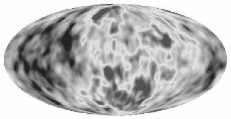
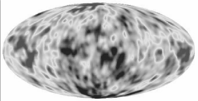
Figure 1: CMB maps for $\Omega_{\Lambda}=0$ (left) and,$\Omega_{\Lambda}=0.7$ (right). The other parameters are as given in the text.

Our result, obtained for a flat FRW Universe with $h=0.72$ and $\Omega_{b}h^{2}=0.002$ is:

$$\frac{G\mu}{c^{2}}=\left(0.695+\frac{0.012}{1-\Omega_{\Lambda}}\right)\times 10^{-6}\,.$$ (4)

The cosmic string simulations all started at $\eta_{0}/4$ and ended at $\eta_{0}$, the conformal time today. This is a lower normalization than obtained in Allen et al. $\!{}^{{\bf?}}$, which is most likely due to the more accurate incorporation of small-scale structure in the string networks.

3.2 Medium to Small Angle Maps

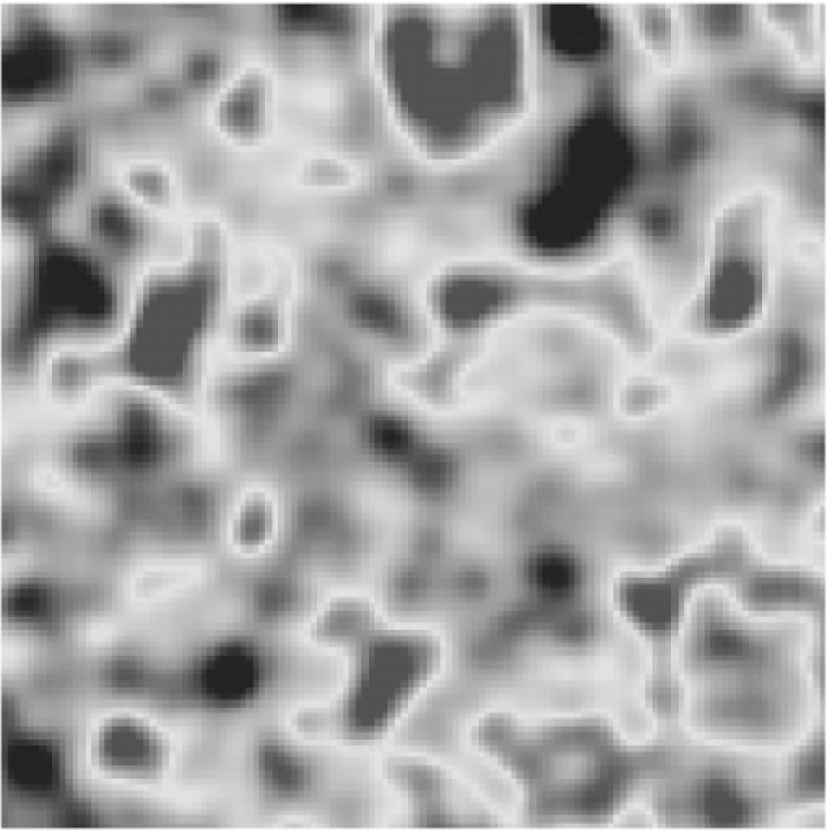
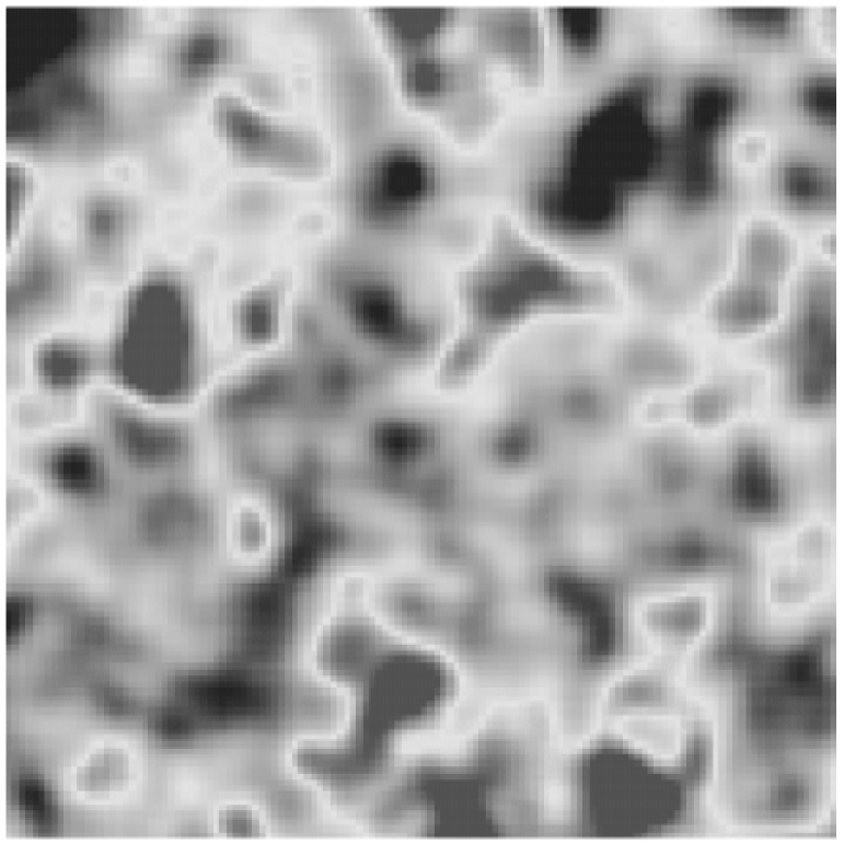
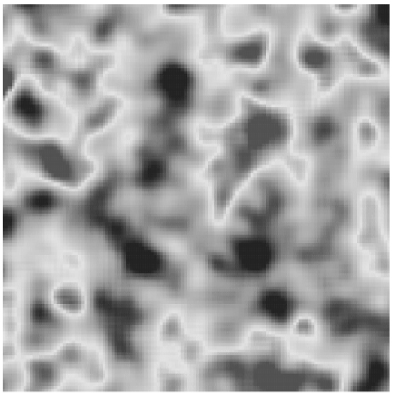
Figure 2: CMB maps of $6.4^{\circ}\times 6.4^{\circ}$, $12.8^{\circ}\times 12.8^{\circ}$ and $25.6^{\circ}\times 25.6^{\circ}$. The parameters are as given in the text.

When studying smaller angular resolution, it is necessary to restrict ourselves to patches of sky. Fig. 2 shows three such maps, each with 16384 square pixels computed for a flat FRW Universe with the same parameters as for the all-sky maps, but with the cosmological constant fixed at $\Omega_{\Lambda}=0.7$. The simulations span different epochs: $\eta_{rec}$ to $4\eta_{rec}$, $2\eta_{rec}$ to $8\eta_{rec}$ and $4\eta_{rec}$ to $16\eta_{rec}$ for the smallest to the largest maps.

We have performed a very basic search for non-Gaussianities and found that the pixel temperature distribution is indeed non-Gaussian, but that the completely diagonal bispectrum is not a good tool to extract this signal. This is most easily seen from Fig. 3. Note that thesevery preliminary results come from simulations with a limited dynamic range, a fact which tends to enhance the signatures of individual strings. Temperature contributions from the higher density of strings at earlier times will tend to push the results towards Gaussianity. Further results will be published elsewhere $\!{}^{{\bf?}}$.

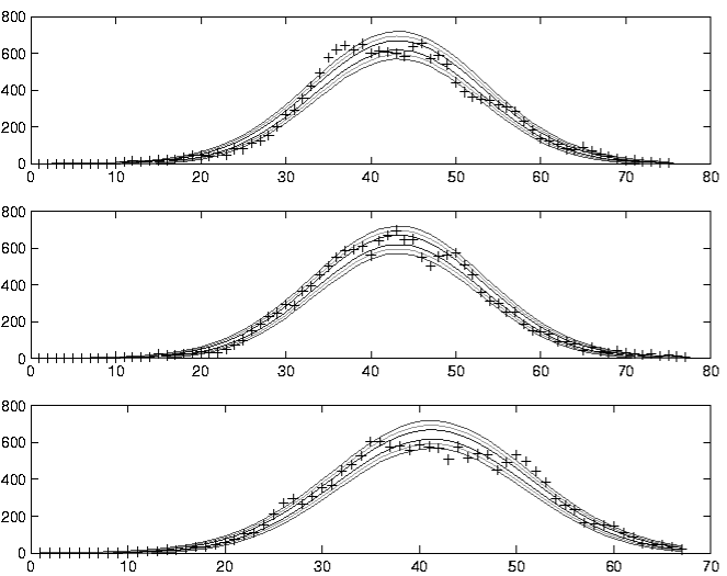
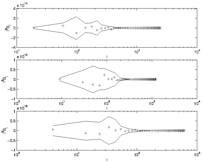
Figure 3: Pixel Temperature distribution for the maps shown in Fig. 2 with the 1-$\sigma$, 2-$\sigma$ and 3-$\sigma$ contours of an ensemble of 1000 Gaussian maps (left) and the diagonal bispectrum for the same maps with the 1-$\sigma$ contours the Gaussian ensemble.

4 Non-Gaussian Inflation

Departures from Gaussianity in inflationnary models can arise in a number of circumstances, for example when there are many fields (e.g Bartolo et al. $\!{}^{{\bf?}}$, Bernardeau & Uzan $\!{}^{{\bf?}}$) or when higher order perturbations are taken into account (e.g. Acquaviva et al. $\!{}^{{\bf?}}$, Maldacena $\!{}^{{\bf?}}$). Other authors have proposed methods to compute non-Gaussian inflationary maps (e.g. Ligouri et al. $\!{}^{{\bf?}}$). Here, we simply adapt the method outlined for cosmic strings (or other causal sources) to inflation. In this case, $q=0$ ; hence, the integral in Eq. 2 is zero as well, which reduces the computation by more than half (there is further reduction in computing time from the fact that the inverts of the fundamental matrices need not be computed, but this is negligeable in comparison). Hence, only the initial conditions need to specified on a grid. These can be obtained from a field simulation of the inflaton $\!{}^{{\bf?}}$.

5 Conclusion and Future Prospects

In this talk, we have reviewed a method to compute maps of the CMB in intrinsically non-Gaussian models. We also presented preliminary results on intermediary angle size CMB maps in the presence of cosmic strings. These maps exhibit some non-Gaussianities, but further analysis may reveal they are not generic. We are currently working on smaller angle high resolution maps from cosmic strings $\!{}^{{\bf?}}$ and non-Gaussian inflation $\!{}^{{\bf?}}$. Hopefully, these two very different scenarios could be easily differentiated by their non-Gaussian signature alone.

Acknoledgements

All the simulations were performed on COSMOS IV, the Origin 3800 supercomputer, funded by SGI, HEFCE and PPARC.

References

References

- [1] C. L. Bennett et al. First year wilkinson microwave anisotropy probe observations: Maps and basic results. ApJS, 148:1, 2003.
- [2] M. Landriau and E. P. S. Shellard. Fluctuations in the CMB induced by cosmic strings: Methods and formalism. Phys.Rev., D67:103512, 2003.
- [3] S. Sarangi and S. H. H. Tye. Cosmic string production towards the end of brane inflation. Phys. Lett., B536:185, 2002.
- [4] B. Allen and E. P. S. Shellard. Cosmic string evolution - a numerical simulation. Phys.Rev.Lett., 64:119, 1990.
- [5] M. Landriau and E. P. S. Shellard. Large angle CMB fluctuations from cosmic strings with a comological constant. astro-ph/0302166; accepted for publication in Physical Review D, 2003.
- [6] B. Allen, R. R. Caldwell, E. P. S. Shellard, A. Stebbins, and S. Veeraraghavan. Large angular scale CMB anisotropy induced by cosmic strings. Phys.Rev.Lett., 77:3061, 1996.
- [7] M. Landriau and E. P. S. Shellard. In preparation.
- [8] N. Bartolo, S. Matarrese, and A. Riotto. Non-Gaussianity from inflation. Phys.Rev., D65:103505, 2003.
- [9] F. Bernardeau and J. P. Uzan. Non-Gaussianity in multi-field inflation. Phys.Rev., D66:103506, 2002.
- [10] V. Acquaviva, N. Bartolo, S. Matarrese, and A. Riotto. Second-order cosmological perturbations from inflation. Nucl.Phys., B 667:119, 2003.
- [11] J. Maldacena. Non-Gaussian features of primordial fluctuations in singlefield inflationary models. JHEP, 0305:013, 2003.
- [12] M. Liguori, S. Matarrese, and L. Moscardini. High-resolution simulations of cosmic microwave background non-Gaussian maps in spherical coordinates. astro-ph/0306248.
- [13] G. Rigopoulos, E. P. S. Shellard, and M. Landriau. In preparation.