The structure of the NGC 1333-IRAS2 protostellar system on 500 AU scales

This paper investigates small-scale (500 AU) structures of dense gas and dust around the low-mass protostellar binary NGC 1333-IRAS2 using millimeter-wavelength aperture-synthesis observations from the Owens Valley and Berkeley-Illinois-Maryland-Association interferometers. The detected $\lambda=3$ mm continuum emission from cold dust is consistent with models of the envelope around IRAS2A, based on previously reported submillimeter-continuum images, down to the 3″, or 500 AU, resolution of the interferometer data. Our data constrain the contribution of an unresolved point source to 22 mJy. The importance of different parameters, such as the size of an inner cavity and impact of the interstellar radiation field, is tested. Within the accuracy of the parameters describing the envelope model, the point source flux has an uncertainty by up to 25%. We interpret this point source as a cold disk of mass $\gtrsim 0.3$ $M_{\odot}$. The same envelope model also reproduces aperture-synthesis line observations of the optically thin isotopic species C³⁴S and H¹³CO⁺. The more optically thick main isotope lines show a variety of components in the protostellar environment: N₂H⁺ is closely correlated with dust concentrations as seen at submillimeter wavelengths and is particularly strong toward the starless core IRAS2C. We hypothesize that N₂H⁺ is destroyed through reactions with CO that is released from icy grains near the protostellar sources IRAS2A and B. CS, HCO⁺, and HCN have complex line shapes apparently affected by both outflow and infall. In addition to the east-west jet seen in SiO and CO originating from IRAS2A, a north-south velocity gradient near this source indicates a second, perpendicular outflow. This suggests the presence of a binary companion within $0{\aas@@fstack{\prime\prime}}3$ (65 AU) from IRAS2A as driving source of this outflow. Alternative explanations of the velocity gradient, such as rotation in a circumstellar envelope or a single, wide-angle ($90^{\circ}$) outflow are less likely.

1 Introduction

Our understanding of the cloud cores that form stars has benefited significantly from the advent over the last years of (sub)millimeter-continuum bolometer cameras. Sensitive, spatially resolved measurements have allowed quantitative testing of models of starless/pre-stellar cores and envelopes around young stars (e.g. Shirley et al., 2000, 2002; Hogerheijde & Sandell, 2000; Motte & André, 2001; Jørgensen et al., 2002; Schöier et al., 2002; Belloche et al., 2002). Not only do these models sketch the evolution of the matter distribution during star formation, they also can serve as ‘baselines’ for interpreting higher resolution observations obtained with millimeter interferometry. Such data address the presence and properties of circumstellar disks during the early, embedded phase (e.g. Hogerheijde et al., 1998, 1999; Looney et al., 2000). This Paper presents millimeter aperture-synthesis observations of continuum and line emission of the young protobinary system NGC~1333-IRAS2, and uses modeling results based on single-dish submillimeter continuum imaging from Jørgensen et al. (2002; Paper I hereafter) to interpret the data in terms of a collapsing envelope, a disk, and (multiple) outflows on 500 AU scales.

The deeply embedded (‘class 0’; Lada, 1987; André et al., 1993) young stellar system NGC~1333-IRAS2 (IRAS 03258+3104; hereafter IRAS2) has been the subject of several detailed studies. It is located in the NGC~1333 molecular cloud, well known for harboring several class 0 and I objects, and was first identified from IRAS data by Jennings et al. (1987). Quoted distances to NGC~1333 range from 220 pc (Černis, 1990) to 350 pc (Herbig & Jones, 1983); here we adopt 220 pc in accordance with Paper I. At this distance the bolometric luminosity of IRAS2 is $16\leavevmode\nobreak\ L_{\odot}$. Submillimeter-continuum imaging (Sandell & Knee, 2001, and Fig. 1 below) and high-resolution millimeter interferometry (Blake, 1996; Looney et al., 2000) have shown that IRAS2 consists of at least three components: two young stellar sources 2A and, 30″ to the south-east, 2B; and one starless condensation 2C, 30″ north-west of 2A. The sources 2A and 2B are also detected at cm wavelengths (Rodríguez et al., 1999; Reipurth et al., 2002).

Maps of CO emission of the IRAS2 region show two outflows, directed north-south and east-west (Liseau et al., 1988; Sandell et al., 1994; Knee & Sandell, 2000; Engargiola & Plambeck, 1999). Both flows appear to originate to within a few arcseconds from 2A (Engargiola & Plambeck, 1999), indicating this source is a binary itself although it has not been resolved so-far. The different dynamical time scales of both flows suggests different evolutionary stages for the binary members, which lead Knee & Sandell (2000) to instead propose 2C (30″ from 2A) as driving source of the north-south flow. It is unclear how well dynamic time scales can be estimated for outflows that propagate through dense and inhomogeneous clouds such as NGC~1333. Single-dish CS and HCO⁺ maps also show contributions by the outflow, especially for CS (Ward-Thompson & Buckley, 2001). The north-south outflow may connect to an observed gradient in centroid velocities near 2A, but the authors cannot rule out rotation in an envelope perpendicular to the east-west flow.

Paper I determined the physical properties of the IRAS2 envelope using one-dimensional radiative transfer modeling of Submillimeter Common User Bolometer Array (SCUBA) maps and the long-wavelength spectral energy distribution (SED). Assuming a single radial power-law density distribution, $\rho\propto r^{-p}$, an index $p=1.8$ and a mass of 1.7 $M_{\odot}$ within 12,000 AU was found (see Table 1 and Fig. 1). Monte-Carlo modeling of the molecular excitation and line formation of C¹⁸O and C¹⁷O observations yield a CO abundance of $2.6\times 10^{-5}$ with respect to H₂, a factor 4-10 lower than what is found in local dark clouds (e.g. Frerking et al., 1982; Lacy et al., 1994).

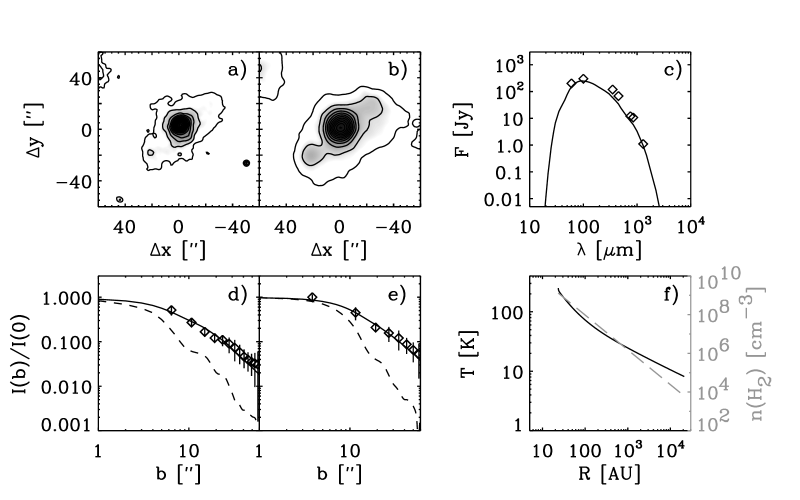
Figure 1: a) and b) SCUBA maps of IRAS2 at 450 and 850 $\mu$m, respectively, centered on IRAS2A. c) Observed SED (symbols) and model fit (solid curve). d) and e) Brightness profiles at 450 and 850 $\mu$m (symbols) and the model fit (solid curve). The dashed curves show the beam profiles. f) Density (dashed line) and temperature (solid line) distributions of best-fit model. See Paper I for details.

Table 1: The parameters for IRAS2 from Paper I.

Distance, $d$	220 pc
$L_{\rm bol}$	16 $L_{\odot}$
$T_{\rm bol}$	50 K
Envelope parameters:
Inner radius ($T=250$ K), $R_{i}$	23.4 AU
Outer radius, $R_{\rm 10K}$a	1.2$\times 10^{4}$ AU
Density at 1000 AU, $n$(H2)	1.5$\times 10^{6}$ cm-3
Slope of density distribution, $p$	1.8
Mass, $M_{\rm 10K}$a	1.7 $M_{\odot}$
CO abundance, [CO/H2]	2.6$\times 10^{-5}$

Notes: ^aThe outer boundary is not well constrained, but taken to be the point where the temperature in the envelope has dropped to 10 K. The mass refers to the envelope mass within this radius.

This Paper presents $\lambda=3$ mm interferometric observations of IRAS2 in a range of molecular emission lines probing dense gas and continuum emission tracing cold dust. It builds on the modeling of Paper I by using it as a framework to interpret the small-scale structure revealed by the aperture-synthesis data. Section 2 describes the observations and reduction methods. Section 3 analyzes the continuum emission, and compares it to the previously derived models. Section 4 presents the molecular-line maps and discusses the physical and chemical properties of the gas in the proximity of IRAS2. Section 5 reports a pronounced north-south velocity gradient around IRAS2A and explores rotation or outflow as possible explanations. Section 6 concludes the Paper by summarizing the main findings. A companion paper (Jørgensen et al., 2003a) presents a detailed study of the bow shock at the tip of the east-west jet from IRAS2 based on single-dish and interferometric (sub)millimeter observations.

2 Observations

2.1 Interferometer data

IRAS2 ($\alpha(2000)=03^{\rm h}28^{\rm m}56\aas@@fstack{s}29$; $\delta(2000)=31^{\circ}14\arcmin 33\aas@@fstack{\prime\prime}93$) was observed with the Millimeter Array of the Owens Valley Radio Observatory (OVRO) between October 5, 1994 and January 1, 1995 in the six-antenna L- and H-configurations. Tracks were obtained in two frequency settings at 86 and 97 GHz, and each track observed alternatingly two fields: the source positions discussed in this Paper and the bow shock at the end of the eastern jet (Jørgensen et al., 2003a). The observed tracks cover projected baselines of 3.1-70 k$\lambda$ at 86 GHz. The observed lines are listed in Table 2, and were recorded in spectral bands with widths of 32 MHz ($\sim 100$ km s^-1). H¹³CO⁺ $1-0$ and CS $2-1$ were observed in 128 spectral channels and the remaining lines in 64 spectral channels. The complex gain variations were calibrated by observing the nearby quasars 0234+285 and 3C84 approximately every 20 minutes. Fluxes were calibrated by observations of Uranus and Neptune. Calibration and flagging of visbilities with clearly deviating amplitudes and/or phases was performed with the MMA reduction package (Scoville et al., 1993).

The millimeter interferometer of the Berkeley-Illinois-Maryland Association (BIMA) observed IRAS2 on November 4-5, 2000, and January 20-21, February 20, and June 5-6, 2001. The array B-, C-, and D-configurations provided projected baselines of 1.7–68 k$\lambda$. The lines of HCO⁺ $J$=1–0, HCN 1–0, N₂H⁺ 1–0, and C³⁴S 2–1 were recorded in 256-channel spectral bands with a total width of 6.25 MHz ($\sim 20$ km s^-1). The complex gain of the interferometer was calibrated by observing the bright quasars 3C84 (4.2 Jy) and 0237+288 (2.3 Jy) approximately every 20 minutes. The absolute flux scale was bootstrapped from observations of Uranus. The rms noise levels are 0.14 Jy beam^-1 in the 24 kHz channels, with a synthesized beam size of $8.2^{\prime\prime}\times 7.5^{\prime\prime}$ FWHM. The data were calibrated with routines from the MIRIAD software package (Sault et al., 1995).

In the reduction, data points with clearly deviating phases or amplitudes were flagged. The maps were cleaned down to 3 times the rms noise using the MIRIAD ‘clean’ routine. The strong continuum of the two central point sources allowed self-calibration, which was applied and used to correct the spectral line data. The naturally weighted continuum observations typically had rms noise better than 1$\times 10^{-3}$ Jy beam^-1 with half power beam widths (HPBW) of $\approx$ 3″ for the OVRO observations and $\approx$ 8″ for the BIMA data (see Table 3). Table 2 lists the details of the line observations.

Table 2: Line data of IRAS2 discussed in this Paper.

Molecule	Line	Rest freq.	Observed with
CH3OH	$2_{1}-1_{1}$	97.5828	OVRO
CS	$2-1$	97.9810	OSO, OVRO
	$3-2$	146.9690	IRAM 30m
	$5-4$	244.9356	IRAM 30m, JCMTb
	$7-6$	342.8830	JCMTb
C34S	$2-1$	96.4129	IRAM 30m, BIMA
	$5-4$	241.0161	JCMT
HCN	$1-0$a	88.6318	OSO, BIMA
H13CO+	$1-0$	86.7543	OSO, OVRO
HCO+	$1-0$	89.1885	OSO, BIMA
N2H+	$1-0$a	93.1737	OSO, BIMA
SiO	$2-1$	86.8470	OVRO
SO	$2_{2}-1_{1}$	86.0940	OVRO
SO2	$7_{3,5}-8_{2,6}$	97.7023	OVRO

Notes: ^aHyperfine splitting observed in one setting. ^bArchival data.

2.2 Single-dish data

Using the Onsala 20 m telescope (OSO) a number of molecules were observed towards IRAS2A in March 2002. These are listed in Table 2. We also include line data from Jørgensen et al. (2002, 2003b) obtained with the IRAM 30m and James Clerk Maxwell (JCMT) telescopes, and spectra taken from the JCMT archive. The lines were converted to the main beam antenna temperature scales using the appropriate efficiencies, and low-order polynomial baselines were fitted and subtracted.

3 The continuum emission

The 3 mm continuum images clearly show the two components 2A at ($-9^{\prime\prime}$, $+3^{\prime\prime}$) and 2B at ($+14^{\prime\prime}$, $-18^{\prime\prime}$) (Fig. 2). Table 3 lists the results of fits of two circular Gaussians to the visibility data. Consistent with Looney et al. (2000), 2A is the stronger of the two. Differences in detected fluxes between the OVRO and BIMA data sets indicate that the emission is extended, and varying amounts are picked up by the respective $(u,v)$ coverages of the arrays. Emission from the third source 2C, north-west of 2A, is not detected, supporting the suggestion that it has not yet formed a star and lacks a strong central concentration.

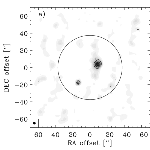
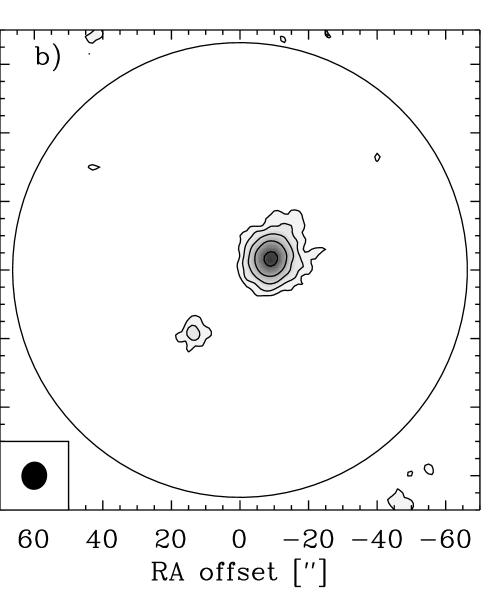
Figure 2: Maps of continuum emission at 86–89 GHz from OVRO (a) and BIMA (b). Offsets are with respect to the pointing center of $\alpha(2000)=03^{\rm h}28^{\rm m}56\aas@@fstack{s}29$ and $\delta(2000)=31^{\circ}14\arcmin 33\aas@@fstack{\prime\prime}93$. Contours are shown at 3$\sigma$, 6$\sigma$, 12$\sigma$, 24$\sigma$ and 48$\sigma$, where $\sigma$ is the RMS noise level of Table 3. The filled ellipses in the lower left corner of the panels indicate the synthesized beam sizes; the large circles show the 50% sensitivity levels of the primary beams.

Table 3: Results of fits to the visibilities.

	OVRO	BIMA
RMS (Jy beam-1)	1.0$\times 10^{-3}$	0.9$\times 10^{-3}$
Beam	3.2″$\times$2.8″	8.2″$\times$7.5″
	IRAS2A
$F_{\rm tot}$ (Jy)	$0.035$	$0.040$
X-offset (″)	$-9.17$	$-8.92$
Y-offset (″)	$3.67$	$3.10$
	IRAS2B
$F_{\rm tot}$ (Jy)	$0.012$	$0.014$
X-offset (″)	$13.66$	$13.78$
Y-offset (″)	$-17.51$	$-18.37$

Notes: IRAS2A is marginally resolved, whereas IRAS2B is unresolved.

3.1 A model for the continuum emission

The different detected fluxes from OVRO and BIMA in Table 3 and comparison of the interferometer images of Fig. 2 and the SCUBA images of Fig. 1 clearly show that the arrays have resolved out significant amounts of extended emission because of their limited $(u,v)$ coverage. The envelope model (density, temperature, dust emissivity as function of wavelength) by Paper I predicts sky-brightness distributions at 3 mm, and fluxes in the interferometer beams after sampling at the actual $(u,v)$ positions and subtracting the contribution from 2B. This latter subtraction of the Gaussian fit to 2B only affects the results minimally, indicating that 2B is well separated from and much weaker than 2A. Fig. 3 compares the predicted flux as function of projected baseline length with the data. In addition to the model envelopes, we have included as free parameter the flux of an unresolved point source ($<3\arcsec$). Because a point source contributes equally on all baselines, this addition corresponds to a vertical offset of the model curve in the plots. Such offsets are apparent in both OVRO and BIMA data, and a point source flux of 22 mJy at 3 mm provides an adequate fit to the data when added to the model envelopes.

Figure 3: Visibility amplitudes of the observed continuum emission from the BIMA (upper panel) and OVRO (lower panel) observations as a function of projected baseline length in k$\lambda$ centered at the position of IRAS2A. The data are plotted as filled symbols with 1$\sigma$ error bars, the continuous lines indicate the predictions from the continuum model of Paper I with the same $(u,v)$ sampling as the observations - respectively with (solid) and without (dashed) an unresolved compact source of 22 mJy added to the model. The dotted histogram indicates the zero-expectation level: the expected amplitude signal due to noise alone in the absence of source emission.

The inferred point source flux is consistent with Looney et al. (2003), who find a 20 mJy source at 2.7 mm associated with IRAS2A. For reasonable assumptions about the spectral index of the point source ($\alpha$=2–4 if thermal) this component does not contribute significantly to the flux in the much larger SCUBA beams, and therefore does not invalidate the SCUBA-based envelope models. The thermal nature of the point source is supported by detection of 2A at a flux of 0.22 mJy at 3.6 cm and a resolution of 0.3″ with the VLA (Reipurth et al., 2002). This yields a spectral index of 1.9 between 3.6 cm and 3.3 mm, consistent with optically thick thermal emission. A similar conclusion was reached by Rodríguez et al. (1999) based on the spectral index from VLA observations of IRAS2A at 3.6 and 6 cm.

Assuming that the point source emission is optically thin and thermal, the inferred flux of 22 mJy corresponds to a dust mass of $3.3\times 10^{-3}$ $M_{\odot}$ if we adopt an average temperature of 30 K and a emissivity per unit (dust) mass at 3.5 mm of $\kappa=0.24$ cm² g^-1 from extrapolation of the opacities by Ossenkopf & Henning (1994) for grains with thin ice mantles as was assumed in the envelope models in Paper I. With a standard gas-to-dust ratio of 100, the total mass is 0.33 $M_{\odot}$. If the emission is optically thick as the spectral index indicates, this is in fact a lower limit to the mass. The favored explanation for this compact mass distribution is a circumstellar disk.

3.2 Parameter dependency of the continuum model

To test the validity of the envelope model a number of parameters were varied within the constraints set by the modeling of the SCUBA observations (Fig. 4). The uncertainty in the power-law index from the SCUBA model of Paper I is $\pm 0.2$. Over this range of density slopes we find central point source fluxes of $22\pm 4$ mJy, with a clear degeneracy between the slope of the density profile and the flux of the central point source. This is similar to what Harvey et al. (2003) find in a detailed analysis of high-resolution millimeter continuum observations of the class 0 object B335. Both BIMA and OVRO data sets are fitted well within the uncertainties using the density profile slope from the SCUBA data, although the actual best fit model to the OVRO data has a slightly steeper density slope ($p=1.9$) and a lower point source flux. The interferometry data cannot constrain the slope of the density profile further than its uncertainty from the SCUBA model. So although the data can be fitted with a single power-law density envelope from the scales probed by the SCUBA observations down to the scales probed by the interferometry observations, a steepening or flattening of the density profile at small scales cannot be ruled out.

Figure 4: Visibility amplitudes of the observed BIMA continuum emission as in Fig. 3 compared to various input models centered at the position of IRAS2A. Upper panels: a) models with changing steepness of the density profile. b) test of different values of the outer radius and inclusion of the interstellar radiation field. Models with an outer radius 3 times larger than the model from paper I (i.e. 36000 AU) are shown. Lower panels: c) fit to the inside-out collapse model of Shu (1977) with parameters constrained independently by molecular line observations and SCUBA continuum observations. d) models with changing size of the inner radius.

Harvey et al. (2003) find that the uncertainty in the central point source flux dominates over uncertainties in other model parameters such as external heating by the interstellar radiation field (ISRF), wavelength dependence of the dust emissivity, outer radius of the envelope, and deviations from spherical symmetry (e.g., an evacuated outflow cavity). Because our interferometer data only sample the inner regions, they are not sensitive to variations in the outer radius or inclusion of heating by the ISRF. The latter hardly affects the temperature structure because the source is relatively luminous and dominates the heating as is seen in Fig. 5.

Figure 5: Temperature profile in the outermost region of the envelope without (solid line) and with (dashed line) contributions from the interstellar radiation field. The dotted line indicates the temperature of 10 K corresponding to the envelope outer radius (Paper I).

In similar studies to that presented in Paper I, Shirley et al. (2002) and Young et al. (2003) modeled the SEDs and brightness profiles from SCUBA observations of protostellar sources using 1D radiative transfer, assuming power-law density profiles and solving for the temperature structure. Two differences exist, however, in the approaches taken in these two papers and our Paper I: Shirley et al. and Young et al. included contributions to the heating of the envelope by the external interstellar radiation field and adopted outer envelope radii significantly larger than those set by the 10 K boundary used in Paper I. For the sources common to the two samples, Shirley et al. found on average steeper density profiles than ours for the class 0 objects whereas Young et al. found similar density profiles to ours for the class I objects. Young et al. suggested that the disagreement for the class 0 objects and agreement for the class I objects was due to a combination of neglect of the ISRF and an underestimate of the sizes of the envelopes in Paper I: while inclusion of the ISRF will indeed tend to steepen the derived density profile, an overestimate of the outer radius (by factors of 2 or more) will tend to flatten the derived profile. As illustrated above, however, these parameters have negligible impact on the IRAS2 envelope structure. It is therefore interesting to note the agreement in slope between the interferometer and SCUBA continuum observations, in contrast to the discussion of B335 by Harvey et al. (2003). Comparing to the results of Shirley et al. (2002), Harvey et al. found a slightly flatter density profile when modeling the interferometer observations. While uncertainty in the outer radius and ISRF may lead to only small departures for the interferometry data, it can lead to systematic changes in the slope of derived power-law density profile from the SCUBA observations of $\simeq 0.2$. This could explain the differences between the density profiles from the interferometry and SCUBA data for B335.

Our envelope model is entirely based on SCUBA data, and the interferometer fluxes serve only to constrain any point source flux. The robustness of that constraint depends on the assumption that the envelope model can be extrapolated down to scales much smaller than the SCUBA resolution (4″= 900 AU). In Paper I the inner radius is fixed at a temperature of 250 K which occurs at $R=22$ AU, but it was argued that this is not determined by the data. The size of any inner cavity is expected to affect the interferometer data since these sample small scales: a larger adopted cavity would result in a higher inferred point source flux to compensate for the reduced small-scale emission. Fig. 6 plots this ‘required’ point source flux against inner cavity size. The point source flux increases from 22 mJy for cavities $<25$ AU to $\approx 27$ mJy for cavities $\gtrsim 200$ AU (1″). The interferometer data would resolve cavities larger than this and a point source could no longer compensate for the removed emission.

Figure 6: Derived point source flux plotted against size of the inner envelope cavity.

Turning this reasoning around, the inferred point source could be due to an increase in envelope density on small scales, as opposed to a circumstellar disk in an envelope cavity. Assuming a temperature of 150 K appropriate for the envelope scales unresolved by the interferometers instead of the 30 K assumed for the disk, one derives a mass of 0.06 $M_{\odot}$. For comparison the mass of the single power-law density model within 150 AU is only 0.008 $M_{\odot}$. So to explain the detected flux an increase in density by almost an order of magnitude is needed, which seems unlikely.

The model from Paper I assumes that the envelope is heated by a stellar blackbody of 5000 K at the center. If, as is argued above, the star is surrounded by a disk that reprocesses a significant fraction of the stellar light, the input spectrum shifts to longer wavelengths. To investigate the effect on the envelope’s temperature structure, Fig. 7 compares the SEDs of the original model and a model where the central star is surrounded by a 200 AU outer radius, 0.33 $M_{\odot}$ disk. The disk follows the descriptions of Chiang & Goldreich (1997) and Dullemond et al. (2001), and the envelope’s inner cavity has been increased to 200 AU in radius so that it encompasses the disk. As a result, the temperature at the inner edge of the envelope drops from the original 250 K (at 22 AU) to 75 K (at 200 AU). The radiative transfer code DUSTY produces the envelope’s temperature distribution and emergent SED using the star+disk spectrum as heating input, similar to the calculations of Paper I for the star-only spectrum. The comparison in Fig. 7 shows that the SEDs between 60 $\mu$m and 1.3 mm are unchanged. Our derived envelope parameters are therefore unaffected by the exact form of the input spectrum. The departures grow larger at the shorter wavelengths (2–20 $\mu$m) and may be observable with, e.g., SIRTF. It is not surprising that the SEDs are most different at these wavelengths. Flared disk models such as those of Chiang & Goldreich (1997) are specifically invoked to explain so-called ‘flat-spectrum’ sources. Their superheated surface layers ‘flatten’ the SED of these star+disk systems by boosting the 2–20 $\mu$m emission. It is not obvious that such a description of the disk is valid for early, deeply embedded objects, such as IRAS2A. Still, the important point here is that the influence of the disk on the observed SED is likely to be negligible at the wavelengths where the envelope model is constrained.

Figure 7: Changes of the emerging SED due to inclusion of a 200 AU outer, 0.3 $M_{\odot}$ disk: in the upper panel the SEDs from the star + envelope (solid line) and star + envelope + disk models (dashed line) are compared. In both models the central star is represented by a 5000 K blackbody. In the lower panel the ratio between the models are shown - the typical 20% error-level in the flux calibration is illustrated by the solid rectangle.

3.3 A collapse model for the continuum emission

As demonstrated by Hogerheijde & Sandell (2000), Shirley et al. (2002), and Schöier et al. (2002) models other than a density power law can also fit continuum observations, in particular the inside-out collapse model of Shu (1977). These authors conclude that a collapse model can provide an equally good fit as power-law models, with the caveat by Shirley et al. (2002) that collapse models only fit their class 0 objects for sufficiently low ages where this model is well approximated by a single power law on the scales resolved by SCUBA. Schöier et al. (2002) and Shirley et al. (2002) find that continuum and line data sets sometimes give discrepant collapse model fits to the same sources, with line data favoring higher ages than continuum data.

Fitting the Shu (1977) inside-out collapse model to the SCUBA data for IRAS2 gives best fit values of $a=0.3$ km s^-1 and $t=1.7\times 10^{4}$ years (see Fig. 8) with the quality of the fits essentially identical to those of the single power-law models. This collapse model also fits the BIMA and OVRO data if a point source of 25 mJy is introduced.

Figure 8: Fits to the SCUBA observations with a inside-out collapse model with an isothermal sound speed, $a$, of 0.3 km s^-1 and an age of $1.7\times 10^{4}$ years.

The integrated CS and C³⁴S line intensities were fitted independently with the collapse model using detailed radiative transfer as in Schöier et al. (2002) for a constant fractional abundance with radius. The uncertainties in the line fluxes are assumed to be 20% and for each model the $\chi^{2}$-estimator is used to pick out the best model and estimate confidence levels for the derived parameters. Interestingly, the fits to the CS and C³⁴S lines (Fig. 9) give identical parameters to those derived from the dust modeling, in contrast with the other sources (e.g. Shirley et al., 2002; Schöier et al., 2002).

Figure 9: Constraints on the inside-out collapse model derived from the CS and C³⁴S line intensities, assuming CS and C³⁴S abundances of 1$\times 10^{-9}$ and 1$\times 10^{-10}$ respectively found in the single power-law density model. The inferred age and sound speed agree well with those derived from the continuum data.

The identical fits to the line intensities and continuum observations and success of both collapse and power-law density models illustrates the low age inferred for IRAS2: the collapse expansion radius in the inside-out collapse model is for the envelope parameters located at $\approx 4\arcsec$ and therefore not directly probed by the SCUBA continuum maps. Likewise the CS lines predominantly probe the outer regions of the envelopes where the density profile in the collapse model for the low age of IRAS2 essentially is a power-law. This also explains why a slightly higher point source flux is obtained with the collapse model than the power-law density model: inside the collapse expansion radius the density profile flattens in the collapse model, lowering the mass and thereby the flux towards the unresolved center of the envelope. This is compensated by increasing the point source flux when modeling the interferometer observations.

In summary, the interferometer continuum data are well described by the same 1.7 $M_{\odot}$ envelope models that fit the SCUBA data. Power-law descriptions for the density and inside-out collapse model fit the data equally well. They indicate the presence of a $F_{\rm 3\,mm}\approx$ 22 mJy point source, presumably a $\gtrsim$ 0.33 $M_{\odot}$ circumstellar disk. Uncertainties associated with the envelope model are reflected in the accuracy of the point source flux, which may vary by up to 25% from the quoted value. The next section describes the line emission in this context.

4 Line emission

4.1 Morphology

Fig. 10-11 shows the integrated intensity maps of all lines detected with BIMA (HCN, HCO⁺, N₂H⁺, C³⁴S) and OVRO (CS, H¹³CO⁺, SO, and CH₃OH). Velocity centroid images are shown for CS, HCN and HCO⁺ in Fig. 12. Emission of SiO and SO₂ was not detected toward the source position. The images from BIMA show more extended structure than those from OVRO because of the different $(u,v)$ coverage of the two arrays. All detected lines have a peak near the object 2A, and most show a peak near 2B. The non-detections of SO and CH₃OH near 2B are likely due to limited sensitivity given the low signal-to-noise of these lines toward 2A. Only the non-detection of N₂H⁺ toward 2B is highly significant: emission in this line appears to avoid 2B. The extended emission picked up by BIMA shows three components. A roughly north-south ridge seen in HCN, HCO⁺, and N₂H⁺; emission along the east-west outflow in HCO⁺ and, at the tip of the eastern jet at the edge of the image, in HCN; and an extended peak in N₂H⁺ around the continuum position 2C. Interestingly, N₂H⁺ also seems to avoid the east-west outflow and appears almost anti-correlated with HCO⁺.

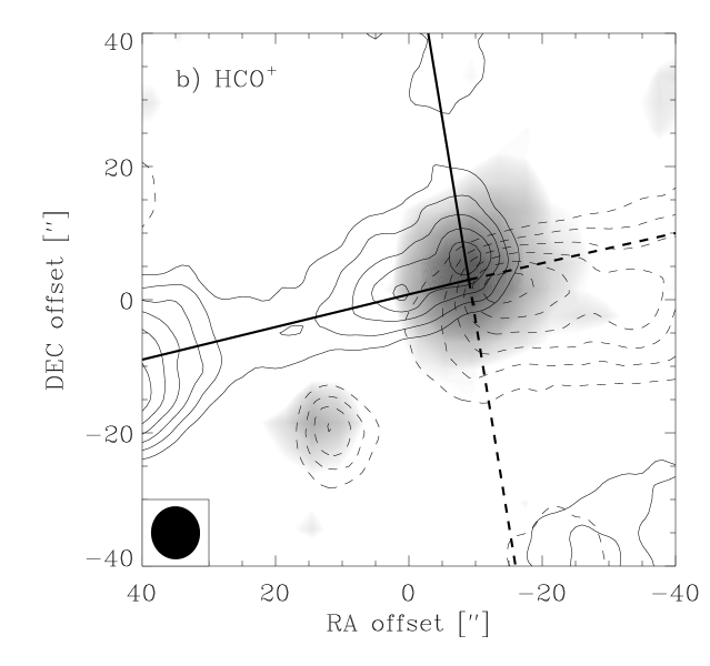
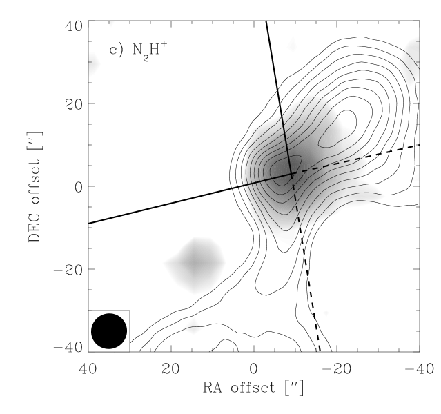
Figure 10: Integrated line emission from the BIMA observations for a) HCN, b) HCO⁺, c) N₂H⁺and d) C³⁴S plotted over the 3 mm continuum maps (grey-scale). The outflow axes have been marked with straight lines with the red part being solid and blue part being dashed. For HCN and HCO⁺ the emission has been integrated over the red and blue parts of the line (3 to 7 km s^-1 and 9 to 13 km s^-1) shown as the dashed and solid lines, respectively. For N₂H⁺ and C³⁴S the total integrated emission is presented, in the case of N₂H⁺ integrated over the main group of hyperfine lines. For C³⁴S the contours are presented in steps of 3$\sigma$, for HCN and HCO⁺ in steps of 5$\sigma$ and for N₂H⁺ in steps of 7$\sigma$.

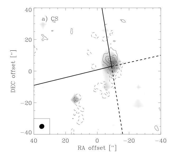
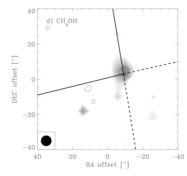
Figure 11: Integrated line emission from the OVRO data, showing a) CS, b) H¹³CO⁺, c) SO and d) CH₃OH. CS is integrated over blue (5 to 9 km s^-1; dashed contours) and red (9 to 13 km s^-1; solid contours) parts of the line with contours in steps of 3$\sigma$. For the other molecules lines have been integrated from 7 to 11 km s^-1 and contours are given in steps of 2$\sigma$. The grey-scale indicate the 3 mm continuum maps.

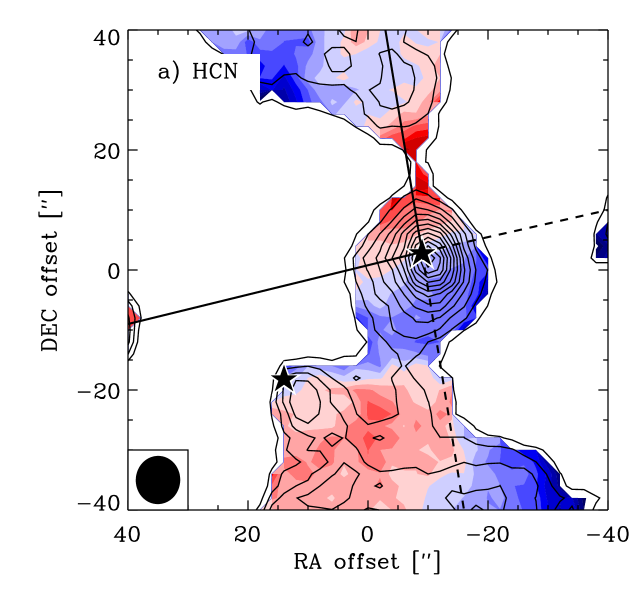
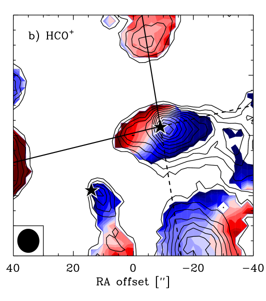
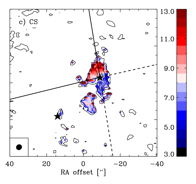
Figure 12: First order moment (velocity) maps of the a) HCN, b) HCO⁺ (BIMA) and c) CS emission (OVRO). Each map has been overplotted with the total integrated emission in steps of 3 $\sigma$ (solid line contours). The outflow axes have been marked by lines and IRAS2A and IRAS2B continuum sources by stars.

The intensity ratio of 1.5:2.7:4.7 of the N₂H⁺ hyperfine lines suggest that the emission is optically thin and close to LTE, where the ratio would be 1:3:5. Relative to the 450 $\mu$m emission from SCUBA that traces cool dust, the N₂H⁺ emission is strongest around 2C, lower around 2A, and absent toward 2B as illustrated in Fig. 13. In a study of dark cloud cores, Bergin et al. (2001, 2002) find that N₂H⁺ has a large abundance deep inside the clouds and a lower abundance in the exterior regions. This trend is opposite to that of CO, which is often highly depleted deep inside cores. Bergin et al. argue that N₂H⁺ is effectively destroyed through reactions with CO, and therefore is only present at high abundance where CO is depleted. This scenario can also explain the relative distribution of N₂H⁺ in 2C, 2A, and 2B: in the starless core 2C temperatures are low and CO is highly depleted, resulting in strong N₂H⁺ emission; in 2A the star has already heated the material and some CO has been released, reducing the N₂H⁺ abundance and emission; the evolved core 2B has been thoroughly heated by the star, and most N₂H⁺ has been effectively destroyed by the released CO. This hints at triggered star formation with the sources lining up from southeast to northwest in evolutionary order, with 2B older than 2A, and 2A older than 2C.

Figure 13: The contrast between the N₂H⁺ and SCUBA emission: the N₂H⁺emission divided by the 450 $\mu$m continuum emission (normalized) along a straight line with a position angle of 45^∘ through IRAS2A (solid line) and the 450 $\mu$m continuum emission in the same positions (dashed line).

Several molecules only show emission in a very narrow velocity range around the systemic velocity of the cloud of $\sim 8$ km s^-1: H¹³CO⁺, SO, CH₃OH, N₂H⁺, and C³⁴S. Others show pronounced gradients in a north-south direction within $\approx$ 20″ from IRAS2A (HCN, HCO⁺, CS) and along the east-west outflow (most clearly in HCO⁺). Whether the north-south gradient around 2A is rotation in a circumstellar envelope or is related to the north-south outflow seen on larger scales is addressed in Section 5. To asses the amount of recovered flux as function of velocity, Fig. 14 compares single-dish spectra with interferometer spectra averaged over the single-dish beam size and converted to the antenna-temperature intensity scale. The interferometer recovers at most 17% of the emission, and much less in many cases. Apart from a scaling factor, the line shapes of C³⁴S, N₂H⁺, and H¹³CO⁺ are similar in the interferometer and single-dish spectra, implying that although the interferometers picked up only the more compact emitting structures, only small velocity gradients can be present within the envelope itself. Deep self-absorption apparent in HCO⁺, HCN, and CS near the systemic velocity indicates that surrounding cloud material is optically thick and entirely resolved out. The velocity structure seen in these lines therefore only reflects material at relatively extreme red- and blue-shifts.

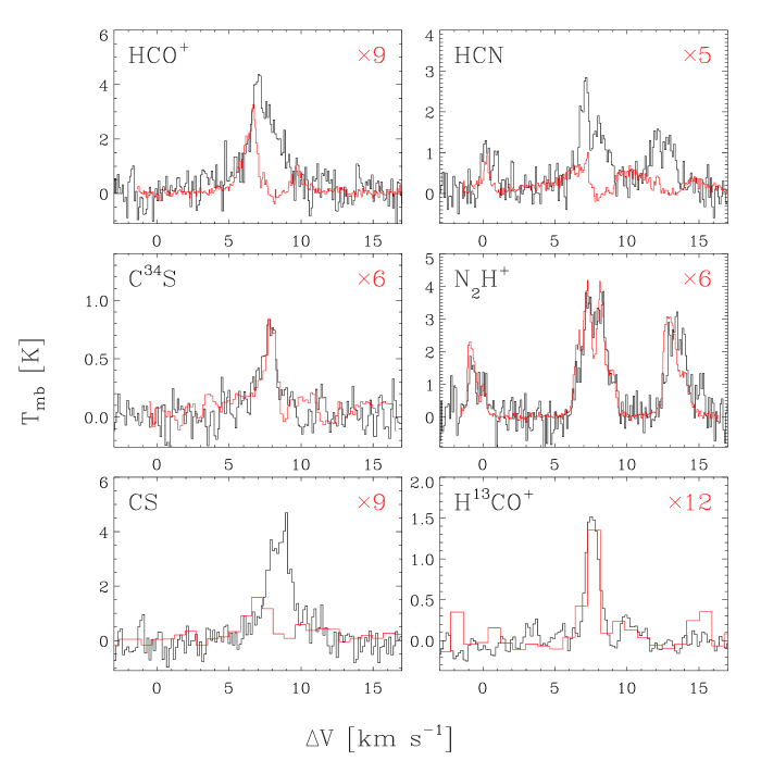
Figure 14: Comparison between the single-dish observations (dark) and corresponding spectra from the interferometer observations restored with the single-dish beam (red). The spectra from the interferometry observations have been scaled by the factors indicated in the upper right corner (factors 5–12) to include all spectra in the same plots.

4.2 Envelope contributions to the line emission

The available envelope model can help explain the interferometric line data, by separating the expected emission of the envelope from other components. We adopt the power-law envelope model of Sect. 3, and fix the molecular abundances from fitting the integrated intensities of single-dish observations of optically thin isotopes. Table 4 lists the derived abundances. Jørgensen et al. (2003b) discuss this method in greater detail and compare the results for a larger sample. With these abundances, the molecular excitation is solved using the code of Hogerheijde & van der Tak (2000) and the emergent sky-brightness distribution calculated. For comparison with the interferometer data the sky-brightness distribution was sampled at the $(u,v)$ positions of the data. The resulting visibilities were then inverted, cleaned, and restored in a similar way as the data.

Table 4: Abundances in the 1D static envelope model derived from of single-dish line observations. For details see Jørgensen et al. (2003b).

Molecule	Abundance ([X/H2])
C34S	1.4$\times 10^{-10}$
CS	1.3$\times 10^{-9}$
H13CO+ (all except 1-0 line)	4.3$\times 10^{-11}$
H13CO+ (1-0 line)	8.0$\times 10^{-11}$

Fig. 15 compares the observed and modeled line emission for C³⁴S. The upper panel shows a comparison between the model and the single-dish observations (upper spectrum) and the interferometry data convolved with the single-dish beam (lower spectrum). In the lower panel the visibilities are plotted as a function of projected baseline length. Both comparisons show that the model works very well in describing the interferometry and single-dish line observations simultaneously and reproduces the emission distribution at the observed scales. This has two implications. First, that optically thin species such as C³⁴S trace material in the envelope and are well described by the model derived from the continuum observations. Second, for species such as C³⁴S the chemistry is homogeneous at the observed radial scales in the envelope, so that a constant fractional abundance is sufficient to describe the chemistry within the assumptions and uncertainties in the modeling.

For H¹³CO⁺ the situation is a bit more complex. The modeling of the single-dish lines reveal a picture similar to that of the CO isotopic species in Paper I; while a constant fractional abundance can describe the line intensities of higher $J$ lines, the intensity of the $J=1-0$ line is underestimated by the model. In Paper I it was suggested that this was due to ambient cloud material being picked up by the larger single-dish beam. The same problem may be an issue for H¹³CO⁺. Fitting the H¹³CO⁺ $J=1-0$ single-dish line alone gives an abundance of 8.0$\times 10^{-11}$. With this abundance, the model can describe the intensity of a spectrum convolved with a beam equivalent to the single-dish observations as illustrated in the upper panel of Fig. 16. The model, however, cannot fit the line profiles simultaneously for the single-dish and interferometry spectra when a constant turbulent broadening is adopted. This is likely caused by the larger single-dish beam picking up the more extended cloud where the velocity distribution may be different. We emphasize, however, that this is a significantly smaller effect than what is seen for, e.g., CS, HCN and HCO⁺ (Fig. 14). It is also seen that the model cannot describe the emission on smaller scales when plotting the visibilities vs. projected baseline length, as illustrated in the lower panel of Fig. 16. If the lower H¹³CO⁺ abundance found from fitting the higher $J$ lines is adopted, the model perfectly reproduces the observed H¹³CO⁺ emission distribution. This discrepancy suggests that the single-dish beam of 44″ picks up the ambient cloud and the envelope around IRAS2B as it also is seen in the H¹³CO⁺ 1–0 interferometry maps. This will contribute to the spectrum extracted from the interferometry cube when convolved with the single-dish beam (e.g. the upper panel of Fig. 16). The good fit to the visibility curve in the lower panel of Fig. 16 indicates that the abundance constrained by the higher excitation single-dish line observations of H¹³CO⁺ is representative of the actual envelope abundance.

It is not possible to account for the observed CS, HCN and HCO⁺ emission within the envelope models. As can be seen in Fig. 17, the CS line intensity is, for example reproduced only at intermediate baselines where also the single-dish line observations are sensitive. On longer baselines the model clearly breaks down and underestimates the observed emission. It is also evident that the pronounced double peak structure seen in interferometry spectra cannot be explained with a simple collapse model alone. This problem will be further explored in the next section.

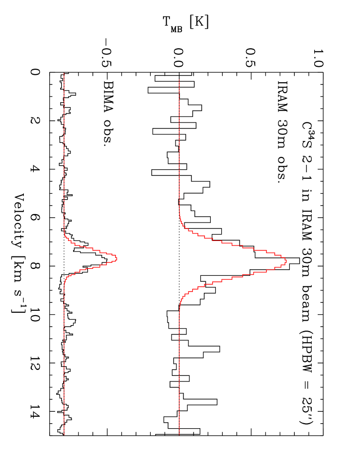
Figure 15: Upper panel: Comparison between the C³⁴S emission from the single-dish observations using the IRAM 30 m telescope with the BIMA interferometry observations (lower spectrum), offset along the $T_{\rm mb}$ axis by -0.8 K and restored with a 25″ beam similar to the single-dish data. The prediction from the 1D static model of the emission brightness distribution from Paper I with abundances derived from single-dish line observations given in Table 4 and sampled at the relevant $(u,v)$ grid has been overplotted on the spectrum in red. Lower panel: visibility amplitude plotted as function of projected baseline length. The predictions from the envelope model with C³⁴S abundance constrained by the single-dish line observations have been overplotted as the solid line. The zero-expectation level is indicated as the dotted histogram.

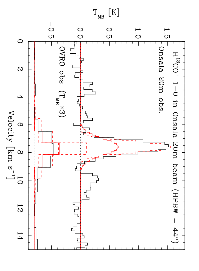
Figure 16: As in Fig. 15, but for H¹³CO⁺ emission as traced by single-dish observations from the Onsala 20m telescope (44″ beam) and interferometry with the OVRO millimeter array. The H¹³CO⁺ interferometer spectra have been scaled by a factor 3 in order to be able to visualize them together with the single-dish observations. The solid line in both panels indicate the model with H¹³CO⁺ abundance constrained by the high $J$ line observations. The dashed line indicate the model constrained by the H¹³CO⁺ $J=1-0$ line. In the lower panel models both with a turbulent broadening of 0.5 and 1.5 km s^-1 have been shown for the abundance constrained by the $1-0$ line. The integrated intensities are the same, however.

Figure 17: Comparison between interferometry observations and envelope model for CS.

5 Velocity structure beyond the envelope

Fig. 18 shows position-velocity diagrams of HCO⁺, HCN, and CS along the north-south velocity gradient apparent in the material within $\approx 20$″ from IRAS2A as seen in Fig. 10-12. The previous section found that the velocity structure in these lines could not be explained by the envelope model with infall. Fitting a linear gradient to the velocity centroid at each offset yields values as given in Table 5 for the three species. It is seen that the fitted velocity gradients agree well and correspond to a weighted average of $1.10\pm 0.23$ km s^-1 arcsec^-1. This gradient may be an overestimate of the actual gradient, because the interferometer predominantly recovers extreme velocities due to resolving out. On the other hand, velocity gradients inferred from single dish observations only are biased toward velocities closer to the rest velocity of the cloud due to the larger beam.

Figure 18: Position-velocity diagrams for a) HCN, b) HCO⁺ and c) CS. The solid line indicates a linear gradient fitted to the centroids for the velocity channel. The hyperfine splitting of HCN is seen as the extension of emission along the velocity axis.

Table 5: Velocity gradient derived through a linear fit to the centroid of the brightness for each velocity channel as indicated in Fig. 18.

Molecule	Velocity gradient
	[km s-1 arcsec-1]
CS	$1.09\pm 0.29$
HCN	$1.00\pm 0.49$
HCO+	$1.25\pm 0.53$

The inferred north-south velocity gradient of 1.10 km s^-1 arcsec^-1, or 1.03$\times 10^{3}$ km s^-1 pc^-1, is two orders of magnitude larger than that inferred by Ward-Thompson & Buckley (2001) from single-dish CS and HCO⁺ observations. This increase in velocity gradient from the spatial scales of the single-dish to the interferometer data is too large to be explained by differential rotation in either a Keplerian structure (expected increase of a factor $\sqrt{10}$) or a magnetically braked core (Basu, 1998) (expected increase of a factor 10). Even if the gradients on single-dish and interferometer scales are unrelated, Keplerian rotation cannot explain our observed velocities since it requires an unrealistically large central mass of 31 $M_{\odot}$.

An alternative explanation for the north-south velocity gradient around IRAS2A is that it is part of the north-south outflow detected on larger scales in CO (Liseau et al., 1988; Engargiola & Plambeck, 1999; Knee & Sandell, 2000). Engargiola & Plambeck (1999) concluded that the origin of this flow lies within a few arcsec from 2A, while Hodapp & Ladd (1995) infer a north-south jet that passes within a few arcsec from 2A from H₂ images. Neither this Paper nor Looney et al. (2000) find evidence for continuum emission from a second source, although it could be below the detection limit or be unresolved ($<0.3\arcsec=65$ AU). The different levels to which HCO⁺, HCN, and CS trace the east-west and north-south flows may reflect differences in shock chemistry as the flows progress through the inhomogeneous cloud environment of IRAS2. This also serves as caution in interpreting differences in the spatial extent of, e.g., CO line wing emission as differences in ‘dynamic time scales’; this presupposes similar environments in which the flows propagate.

Instead of two perpendicular outflows, a single, wide-angle ($90^{\circ}$), northwest–southeast flow could also explain the observed gradients. In this interpretation, what appear to be two independent flows actually trace the interaction of the wide-angle flow with the surrounding material along the sides of the cavity. This scenario is reminiscent of the wide-angle outflow of B5-IRS1 (Velusamy & Langer, 1998). However, in this scenario the jet-like morphology of the shocked region east of IRAS2 (Blake, 1996; Bachiller et al., 1998; Jørgensen et al., 2003a) is difficult to explain.

6 Conclusion

This Paper has shown that the envelope model derived from submillimeter continuum imaging with SCUBA provides a useful framework to interpret interferometric measurements of continuum and line emission. It allows separation of small-scale structures associated with the envelope from small-scale structure in additional elements of the protostellar environment, such as outflows and disks. Our main findings are as follows.

1. Compact 3 mm continuum emission is associated with the two protostellar sources NGC 1333-IRAS2A and 2B; the starless core 2C is not detected, indicating it lacks sufficient central concentration.

2. The 3 mm continuum emission around 2A in the interferometer data is consistent with the extrapolation of the envelope density and temperature distribution to small scales. Changes in the extent of the envelope and inclusion of the interstellar radiation field do not change this conclusion. A density structure as predicted from an inside-out collapse (Shu, 1977) fits the data equally well.

3. The 3 mm continuum data show the presence of a 22 mJy unresolved source, presumably a circumstellar disk of total mass $\gtrsim 0.3$ $M_{\odot}$.

4. Line emission in the optically thin tracers H¹³CO⁺ and C³⁴S is also consistent with the extrapolated envelope model. Since these tracers are optically thin, this suggest that the bulk of the material is well described by the envelope model.

5. Optically thick emission lines of CS, HCO⁺, and HCN only trace a small fraction of the material at velocities red- and blue-shifted by several km s^-1. Emission closer to systemic is obscured by resolved-out large-scale material. The detected emission is closely associated with two perpendicular outflows directed east-west and north-south. This suggests that the source 2A is an unresolved ($<65$ AU) binary.

6. The morphology of the line emission in the maps shows that chemical effects are present. An example is the emission of N₂H⁺ that traces cold material around 2A and that is especially strong toward the starless core 2C. The emission avoids the region around 2B and the outflows. We suggest that the dearth of N₂H⁺ emission is due to destruction through reaction with CO released from ice mantles in warmed-up regions. This indicates an evolutionary ordering 2C–2A–2B, in order of increasing thermal processing of the material.

This work suggests that successful interpretation of the small-scale structure around embedded protostars requires a solid framework for the structure of the surrounding envelope on larger scales. In this framework one can effectively fill in the larger-scale emission that is resolved out by interferometer observations. The submillimeter-continuum imaging by instruments like SCUBA has proved particularly powerful because it does not suffer from chemical effects that make line emission measurements so complex. On the other hand, this very chemistry reflects which physical processes are occurring: e.g., the N₂H⁺ emission that shows the thermal history of the material.

The success of the envelope model in describing the optically thin species, such as C³⁴S and H¹³CO⁺ makes IRAS2 a promising candidate in order to study the relation between the envelope chemistry and the spatial distribution of molecular species. In particular, studies of a larger sample of optically thin molecular lines at arcsecond scale resolution may probe differences in the radial distributions of molecules reflecting the chemistry. IRAS2A is for this purpose a promising target due to the relative simplicity of the central envelope component. High angular resolution, high sensitivity maps may also allow for a more detailed comparison to models for the protostellar collapse in order to possibly address the evolution of low-mass protostars in the earliest stages.