The Luminosity Function of Void Galaxies in the Sloan Digital Sky Survey

Abstract

The Sloan Digital Sky Survey now extends over a large enough region that galaxies in low density environments can be detected. Rojas et al. have developed a technique to extract more than 1000 void galaxies with $\delta\rho/\rho<-0.6$ on scales r $>7h^{-1}$Mpc from the SDSS. In this paper, we present the luminosity function of these galaxies and compare it to that of galaxies at higher densities. We obtain a measurement of the void galaxy luminosity function over the range $-21.5<$ M${}_{\rm r}^{*}<-14.5$ in the SDSS r-band. The void galaxy luminosity function (LF) is well fit by a Schechter function with values of $\Phi^{*}=(0.19\pm 0.04)\times 0.01h^{3}$Mpc^-3, M${}_{\rm r}^{*}$ - 5log$h=-19.74\pm 0.11$ and $\alpha=-1.18\pm 0.13$, where as the LF of the wall galaxy has Schechter function parameters $\Phi^{*}=(1.42\pm 0.03)\times 0.01h^{3}$Mpc^-3, M${}_{\rm r}^{*}$ - 5log$h=-20.62\pm 0.08$ and $\alpha=-1.19\pm 0.07$. The fainter value of M${}_{\rm r}^{*}$ is consistent with the work of Rojas et al. who found that void galaxies were fainter than galaxies at higher densities but the value of $\alpha$ is very similar to that of galaxies at higher densities. To investigate this further, the LF of wall and void galaxies as a function of density is considered. Only the wall galaxies in the highest density regions have a shallower faint end slope. The LF of the void galaxies is also compared to the LF of the wall galaxies with and without similar properties to the void galaxies (color, Sersic index and strength of H$\alpha$ emission). The LF of the bluest, Sersic index $n<2$ and EW(H$\alpha)>5\AA$ wall galaxies is very similar in shape to that of the void galaxies, with only slightly brighter M${}_{\rm r}^{*}$ values and similar values of $\alpha$. The LFs of the red, high Sersic index, low EW(H$\alpha$) wall galaxies have a much shallower slope and brighter M${}_{\rm r}^{*}$ values. The value of $\alpha\approx-1.2$ found from the void galaxy LF is shallower that that found from CDM models, suggesting that voids are not filled with a large population of dwarf galaxies.

1 Introduction

One of the most fundamental properties of a distribution of galaxies is the luminosity function (LF) where $\Phi(L)=dN/dLdV$. Measurements of the galaxy LF have improved over recent years due to the large size of new redshift surveys, such as the 2dF Galaxy Redshift Survey (2dFGRS) and the Sloan Digital Sky Survey (SDSS). For example, Norberg et al. (2002b) measured the $b_{J}$-band LF from a sample of 110,500 galaxies from the 2dFGRS and Blanton et al. (2002) measured the r-band LF from a sample of 147,986 galaxies taken from SDSS.

The samples of galaxies are now large enough that they can be split into subsamples and the properties of different types of galaxies can be studied in more detail. Projects based on 2dFGRS data include Madgwick et al. (2002) who measured the LF as a function of spectral type, Norberg et al. (2002a) who studied the dependence of galaxy clustering strength on luminosity, and Lewis et al. (2002) who studied the environmental dependence of galaxy star formation rates. In the case of the SDSS, Nakamura et al. (2003) have studied the LF as a function of galaxy morphology, Hogg et al. (2002, 2003) have studied the overdensities of galaxy environments as a function of luminosity and color, Gómez et al. (2002) have studied galaxy star-formation as a function of environment and Goto et al. (2003) studied the environment of passive spiral galaxies.

There are many measurements of the LF in many different wavebands and over a wide range of environments. We restrict our discussion to LFs measured from optical surveys that cover wide areas. See de Lapparent (2003) for a comprehensive review of LFs. Most of these analyses have focused on the LF of galaxies found in regions with densities equal or higher to the density around field galaxies (e.g. Loveday et al. 1992; Marzke et al. 1994a, b; Zucca et al. 1997; Ratcliffe et al. 1998; Lin et al. 1996; Folkes et al. 1999; Blanton et al. 2001, 2002; Norberg et al. 2002b). In this paper, we will focus on the LF of galaxies found in extremely underdense environments ($\delta\rho/\rho<-0.6$ measured on scales of $7h^{-1}$Mpc), which we will refer to as void galaxies.

The reason we wish to study the LF of void galaxies is to shed light on the discrepancies between theory and observation. CDM models predict the existence of low mass halos in voids (Dekel & Silk 1986; Hoffman, Silk & Wyse 1992). If these halos contain dwarf galaxies then the void galaxy luminosity function should have a steep faint end slope. However, surveys of dwarf galaxies indicate that they trace the same overall structures as ‘normal’ galaxies (Bingelli 1989) and pointed observations toward void regions have also failed to detect a significant population of faint galaxies (Kuhn, Hopp & Elsässer 1997; Popescu, Hopp & Elsässer 1997). Also, including the effects of photoionization in theoretical models has been shown to restrict galaxy formation, which leads to a LF with a flatter faint-end slope (Benson et al. 2003). However, observationally the shape of the void galaxy LF remains unknown. Grogin & Geller (1999) measured the void galaxy LF for 46 galaxies in regions with density less than half of the mean density (i.e. $\delta\rho/\rho<-0.5$). They found that the LF of void galaxies was quite steep, $\alpha=-1.4\pm 0.5$. This value lies between the steep values predicted by CDM and the shallower values found observationally for galaxies in denser environments.

In this paper we have a sample of $10^{3}$ void galaxies selected from the SDSS from which the void galaxy LF can be measured. Rojas et al. (2003a, b) has already studied the properties of these galaxies. They find that void galaxies are fainter, bluer, have surface brightness profiles more similar to late-type galaxies and that they have higher specific star formation rates. Goldberg et al. (2003 in prep) have also investigated the form of the mass function in voids. They find that the observed mass function is consistent in both shape and normalization with a semi-analytical mass function in an underdense environment with $\delta\rho/\rho<-0.5$. This paper is outlined as follows. In section 2 we describe the SDSS and how void galaxies are selected from it. In section 3 we describe how the LF is estimated and present the results in section 4. In section 5 we consider the LF of different sub-samples of the data, in section 6 we interpret the results and compare to other studies and in section 7 we give conclusions.

2 The Void Galaxy Sample

To obtain a sample of 10³ void galaxies, we use data from the Sloan Digital Sky Survey. The SDSS is a wide-field photometric and spectroscopic survey. The completed survey will cover approximately $10^{4}$ square degrees. CCD imaging of 10⁸ galaxies in five colors and follow-up spectroscopy of 10⁶ galaxies with $r<17.77$ will be obtained. York et al. (2000) provides an overview of the SDSS and Stoughton et al. (2002) describes the early data release (EDR) and details about the photometric and spectroscopic measurements and Abazajian et al. (2003) describes the first data release (DR1). Technical articles providing details of the SDSS include descriptions of the photometric camera (Gunn et al. 1998), photometric analysis (Lupton et al. 2002), the photometric system (Fukugita et al. 1996; Smith et al. 2002), the photometric monitor (Hogg et al. 2001), astrometric calibration (Pier et al. 2003), selection of the galaxy spectroscopic samples (Strauss et al. 2002; Eisenstein et al. 2001), and spectroscopic tiling (Blanton et al. 2003a). A thorough analysis of possible systematic uncertainties in the galaxy samples is described in Scranton et al. (2002). All the galaxies are k-corrected and evolution corrected according to Blanton et al. (2003b) and we assume a $\Omega_{\rm m},\Omega_{\Lambda}$ = 0.3, 0.7 cosmology and Hubble’s constant, $h=H_{o}/100$ km s^-1Mpc^-1 throughout.

Void galaxies are drawn from a sample referred to as sample10 (Blanton et al. 2002). This sample covers nearly 2000 deg² and contains 155,126 galaxies. We use a nearest neighbor analysis to select galaxies that on scales of 7$h^{-1}$Mpc have density contrast, $\delta\rho/\rho<-0.6$ as void galaxies. In the future we wish to identify void galaxies with even lower values of $\delta\rho/\rho$ but with this sample it is not possible. The choice of $\delta\rho/\rho<-0.6$ for the density around void galaxies is also consistent with other definitions of voids. For example the voidfinder of Hoyle & Vogeley (2002) identifies on scales of 7$h^{-1}$Mpc whether galaxies are ‘void’ or ‘wall’ galaxies. The void galaxies can reside in voids reqions but even though 10% of galaxies are classified as void galaxies, the void regions still have average values of $\delta\rho/\rho<-0.9$. Other techniques such as the method of El-Ad & Piran (1997) or use of tessellation techniques such as the Delaunay Tessellation described in Hoyle et al. (2003 in prep.) could also be used to find void galaxies but currently the geometry of the SDSS does not allow these techniques to be used as they require large contiguous volumes. The exact process of selecting the void galaxies is described in detail in Rojas et al. (2003a). We provide a brief overview, as follows:

First, a volume limited sample with z${}_{\rm max}=0.089$ is constructed. This is used to trace the distribution of the voids. Any galaxy in the full flux-limited sample with redshift z$<$z_max that has less then three volume-limited neighbors in a sphere with radius 7$h^{-1}$Mpc and which does not lie close to the edge of the survey is considered a void galaxy. Galaxies with more than 3 neighbors are called wall galaxies. Flux-limited galaxies that lie close to the survey boundary are removed from either sample as it is impossible to tell if a galaxy is a void galaxy or if its neighbors have not yet been observed. This produces a sample of 1,010 void galaxies and 12,732 wall galaxies. These void and wall galaxies have redshifts in the range $0.034\mathrel{\hbox{\hbox to0.0pt{\hbox{\lower 4.0pt\hbox{$\sim$}}\hss}\hbox{$<$}}}z<0.089$ and, more importantly for the LF, the void galaxies have magnitudes in the range $-22<$M${}_{\rm r}<-17.77$, which we show in the left hand plot of figure 1. This sample is referred to as the distant sample.

The SDSS observing schedule is to observe narrow (2.5 degree) but long ($\sim 100$ degree) great circles on the sky. Therefore, there is little nearby volume in the SDSS and all the galaxies lie close to the SDSS boundary. However, the wider angle Updated Zwicky Catalog (Falco et al. 1999) and the Southern Sky Redshift Survey (da Costa et al. 1998) can be used to trace the distribution of voids locally (see figure 1. in Rojas et al. 2003a). Volume-limited samples with approximately the same density as the SDSS volume-limited sample are constructed. These have z${}_{\rm max}=0.025$. We apply the same nearest neighbor analysis and identify a further 194 void galaxies and 2,256 wall galaxies. The absolute magnitude of the galaxies is $-19.7<$M${}_{\rm r}<-13$, shown in the right hand plot of figure 1. This sample is referred to as the nearby sample.

The properties of the galaxies that we are interested in are there magnitudes, colors, surface brightness profiles and star formation rates. The magnitudes that are measured from the SDSS are petrosian magnitudes (Petrosian 1976). More details are given in Stoughton et al. (2002) but basically the petrosian magnitude is the total amount of flux within a circular aperture whose radius depends on the shape of the galaxy light profile, i.e., the size of the aperture is not fixed so galaxies of the same type are observed out to the same physical distance at all redshifts. The colors of the galaxies are found using petrosian magnitudes in two bands. We use the g-r color as the u-band data can be noisy. To estimate the form of the surface brightness profile we use the Sersic index (Sersic 1968) measured by Blanton et al. (2002). The Sersic index, $n$, is found by fitting the functional form $I(r)=I_{0}{\rm exp}(-r^{1/n})$. A value of $n=1$ corresponds to a purely exponential profiles, while $n=4$ is a de Vaucouleurs profile. The final measurement we consider is the star formation rate, as measured by the strength of the H$\alpha$ emission line. We could also consider other lines such as H$\beta$, OII, NII. Rojas et al. (2003b) finds that on average the equivalent widths of void galaxies are larger than the equivalent widths of wall galaxies in all of these lines. As we just want to define a high and low star formation rate sub-samples (see section 5), the choice of the line over the others is not critical.

3 Estimating the Luminosity Function

3.1 Method

Although referred to throughout this paper as the luminosity function, we actually calculate the magnitude function, $\Phi(M)$, which is related to the LF through the relation $\Phi(L)dL=\Phi(M)dM$. To calculate the LF, we use the maximum likelihood approach of Efstathiou, Ellis & Peterson (1988, SWML). Similar results were obtained using the V_max method (Schmidt 1968), apart from at the faint end where the V_max method is known to be a poor estimator due to sample variance.

We measure the LF of the distant and nearby, void and wall galaxies separately. The distant and nearby LFs are combined using an error weighted average of the two measurements in the region of overlap. The LFs of the wall and void galaxy samples are normalized to match the number per square degree of galaxies that would be predicted from the full SDSS sample. Approximately 11/12ths of the galaxies are considered wall galaxies and 1/12th are void galaxies (Rojas et al. 2003a).

To measure $\Phi^{*}$, M${}_{\rm r}^{*}$ and $\alpha$ we $\chi^{2}$-fit the void and wall LFs to a Schechter function. We $\chi^{2}$-fit the Schechter function twice to each LF: The first time, all three parameters are allowed to vary to obtain an estimate of M${}_{\rm r}^{*}$. The second time, we $\chi^{2}$-fit the three parameters again but only over the range M${}_{\rm r}^{*}$-1 $<$ M${}_{\rm r}<$ M${}_{\rm r}^{*}$+5 which means we are fitting the Schechter function to the same part of the LF for each sub-sample. We do this because the wall galaxy LF can be measured over a wider range of magnitudes than the void galaxy LF and thus a comparison between the two LFs might not otherwise be fair. Estimates of $\alpha$ are most sensitive to the range of magnitudes over which the fits are performed. Even so, the values of $\alpha$ found by the restricted range and the full range of magnitudes available agree within 1$\sigma$.

3.2 Errors

We use two methods to estimate the uncertainties in the LF measurements. The first method is that of Efstathiou et al. (1988), which uses the property that the maximum-likelihood estimates of $\Phi$ are asymptotically normally distributed. An alternative is the jackknife method (Lupton 1993). Following Blanton et al. (2001), we construct 18 sub samples of the galaxies. Each sub-sample excludes a different 1/18th of the area of the survey. We measure the LF of each sample and estimate the error via

$${\rm Var}(x)=\frac{N-1}{N}\sum_{i=1}^{N}(x-(\bar{x}))^{2}.$$ (1)

4 Luminosity Functions of Void and Wall Galaxies

In figure 2, we present the LFs of the void and wall galaxies. The first thing to notice is that we are able to measure the LF of void galaxies over a wide range of absolute M_r values, from $-21.5<$M${}_{\rm r}<-14.5$. This is only possible due to the large volume of the SDSS and the way in which void galaxies were found both locally, using the UZC and SSRS2, and at higher redshifts. The amplitudes of the distant and nearby LFs match well in amplitude in the region where they sample the same range of absolute magnitude, as shown in figure 2. In the left hand plot, we show the LFs estimated from the void (lower amplitude) and wall (higher amplitude), distant (solid lines) and nearby (dashed lines) samples. In the right hand side of figure 2, we show a combined void (circles) and wall (triangles) LF. The errors shown come from the method of Efstathiou et al. (1988). The solid lines show best fit Schechter function curves. These are discussed further below.

Sample	$\Phi^{*}$	M${}_{\rm r}^{*}$ - 5log$h$	$\alpha$	$\chi^{2}/\nu$
	$\times$ 0.01$h^{3}$Mpc-3
Void Combined	0.19$\pm 0.04$	-19.74$\pm 0.11$	-1.18$\pm 0.13$	0.9
Void Distant	0.20$\pm 0.08$	-19.68$\pm 0.18$	-0.97$\pm 0.23$	1.1
Void Nearby	0.31$\pm 0.21$	-20.10$\pm 1.90$	-1.25$\pm 0.15$	0.5
Wall Combined	1.42$\pm 0.3$	-20.62$\pm 0.08$	-1.19$\pm 0.07$	1.9
Wall Distant	1.79$\pm 0.6$	-20.40$\pm 0.14$	-1.03$\pm 0.16$	2.3
Wall Nearby	4.20$\pm 1.2$	-18.55$\pm 1.29$	-1.15$\pm 0.12$	0.7

Table 1: Fitting a Schechter function to the void and wall LFs of the combined (distant and near LFs combined into one LF), distant, and near samples. The distant samples alone can constrain $\Phi^{*}$ and M${}_{\rm r}^{*}$ well but cannot place strict limits on $\alpha$, whereas the nearby samples constrain $\alpha$ better.

We compare the errors found via the Efstathiou et al. and jackknife methods in figure 3. Figure 3 shows the fractional error as measured by the two methods for each sample, void/wall, distant/nearby. The errors match each other very well, especially in places where the LF can be accurately measured. The jackknife errors tend to vary more from point to point, whereas the Efstathiou et al. errors follow a smoother trend. As the two methods give consistent results we will only consider the Efstathiou et al. errors in any further analysis.

We $\chi^{2}$-fit a Schechter function to the various LFs as described in section 3. In the case of the void galaxies, the LFs are very well fit with values of $\chi^{2}$ per degree of freedom close to 1. The wall galaxies are less well fit by a Schechter function: the value of $\chi^{2}$ per degree is around 2.5. These values probably reflect the smaller errorbars on the wall galaxy LF more than the fact that the void galaxies have a LF with a shape that more closely resembles a Schechter function.

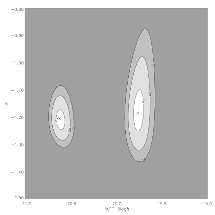
The best fit Schechter function parameters to the combined void and wall galaxy LFs are shown in table 1. The values from the combined void and wall samples are used to calculate the Schechter function curves in figure 2. In figure 4, we fix $\Phi^{*}$, using the value in table 1, and present the contours of $\alpha$ and M${}_{\rm r}^{*}$ found from fitting the combined LFs. The Schechter function parameters found for the combined wall sample are similar to those of Blanton et al. (2001), who obtained $\Phi^{*}=(1.46\pm 0.12)\times 10^{-2}h^{3}$ Mpc^-3, M${}_{\rm r}^{*}$ - 5log$h=-20.83\pm 0.03$ and $\alpha=-1.20\pm 0.03$. We also fit the distant samples and nearby samples independently. In the distant sample cases, the value of $\alpha$ is not well determined. In the nearby sample cases, $\Phi^{*}$ and M${}_{\rm r}^{*}$ are not well fit. This is because the nearby and distant samples alone only probe a narrow range of luminosity. These results are also given in table 1.

It may be possible that the LF and the Schechter function parameters are incorrectly estimated due to the way the nearby and distant samples are matched together. The value of M${}_{\rm r}^{*}$ and $\alpha$ should not be too affected as only the points around M${}_{\rm r}=-17.5$ have little influence on the estimation of these parameters. The overall normalization is most likely to be affected as the points around -17.5 might be underestimated. To see what difference the points in the overlap around M_r=-17.5 have on the estimation of the LF, we ignore the points between $-18<$M${}_{\rm r}<-16.7$ and refit the combined void LF. The Schechter function parameters agree with those found from fitting the whole LF to within 1$\sigma$. Once the SDSS is finished it will cover a larger contiguous area, thus the void galaxies can be detected nearby without the use of the CFA+SSRS2 and the LF estimated from one contiguous sample. The larger number of void galaxies will also make it possible to consider the bivariate distribution of surface brightness and luminosity.

5 Luminosity Function as a function of Density, Color, Profile and H$\alpha$ Line Strength

The sample of void galaxies is large enough that it can be split in half and the LF measured without the uncertainty in the measurement of the LF dominating the LF signal. In figure 5, the LF of the void and wall galaxies is considered as a function of local density. We use the distance to the third nearest neighbor as a measure of the local density and split both the void and wall galaxy samples close to the median value, then measure the LF from these sub-samples.

Sample	$\Phi^{*}$	M${}_{\rm r}^{*}$ - 5log$h$	$\alpha$	$\chi^{2}/\nu$
	$\times$0.01$h^{3}$Mpc-3
Blue	0.90$\pm 0.5$	-20.34$\pm 0.14$	-1.32$\pm 0.11$	1.0
Sersic index $<2$	1.30$\pm 0.6$	-20.02$\pm 0.16$	-1.28$\pm 0.10$	0.9
High EW(H$\alpha$)	0.90$\pm 0.5$	-19.98$\pm 0.17$	-1.32$\pm 0.11$	1.0
Red	0.98$\pm 0.5$	-20.38$\pm 0.12$	-0.73$\pm 0.21$	4.8
Sersic index $>2$	0.98$\pm 0.5$	-20.34$\pm 0.14$	-0.51$\pm 0.32$	8.0
Low EW(H$\alpha$)	1.00$\pm 0.6$	-20.36$\pm 0.14$	-0.55$\pm 0.35$	7.8

Table 2: Fitting a Schechter function to the wall galaxies split by color, Sersic index and strength of the H$\alpha$ emission. The fits are made to the LFs shown in figure 6 and described in section 5.

The void galaxies all have a distance to the third nearest neighbor larger than 7$h^{-1}$Mpc which implies a value of $\delta\rho/\rho<-0.6$ (see Rojas et al. 2003a for details). We split the sample at 8.4$h^{-1}$Mpc which means the lowest density half contains galaxies with $\delta\rho/\rho<-0.75$ and the higher density half has galaxies with $-0.75<\delta\rho/\rho<-0.6$. The wall galaxy sample has an median distance to the third nearest neighbor close to 4$h^{-1}$Mpc. The wall galaxies are split here which means the lower density wall sample has values of $-0.6<\delta\rho/\rho<1$ and the higher density wall galaxy sample has values of $1<\delta\rho/\rho$. In this case only, we also sparsely sample the wall galaxy samples to contain 500 galaxies which is the number of void galaxies in each sample so that the signal in the void and wall galaxies is comparable.

We find that the LFs of the high and low density void samples and the low density wall sample are similar. There is a trend towards brighter values of M${}_{\rm r}^{*}$ - 5log$h$ ($\sim-19.70,-19.80,-20.20,\pm 0.15$ respectively) with increasing density but the faint end slopes are quite similar ($\sim-1.15\pm 0.20$). These LFs are very similar to the shape of the LF of the full void galaxy sample, but with a factor of two lower amplitude. The LF of the wall galaxies in the highest density sample, however, has a somewhat different shape: the faint end slope, $\alpha$, is shallower ($-0.92\pm 0.20$) and M${}_{\rm r}^{*}$ - 5log$h$ is brighter ($-20.40\pm 0.15$).

To investigate the shape of the LF further, we would like to study the void galaxy LF as a function of photometric and spectroscopic parameters such as color, surface brightness profile (SBP), and line widths. However, as shown in Rojas et al. (2003a), the void galaxies only have a narrow range of these properties - they are blue, have small $n<2$ Sersic indices and have strong equivalent widths (Rojas et al. 2003b, in prep). Instead, we consider the wall galaxies and split these into one sample that has properties similar to the void galaxies and one that does not, i.e. we split on color at g-r=0.75, Sersic index at $n=2$ and H$\alpha$ equivalent width of 5 Å, and measure the LF of each sample of wall galaxies. These values are close to but not exactly the median value.

In each of the panels in figure 6, we show the LF of the full void and wall galaxy samples, as shown in figure 2, the LF of the wall galaxies with properties similar to void galaxies (open circles), and the LF of the wall galaxies with properties dissimilar to void galaxies (filled circles). We also show the void galaxy LF multiplied by a factor of 11 to approximately match the amplitude of the wall galaxy LF as there are $\sim$11 times as many wall galaxies as void galaxies. We show the blue vs. red wall galaxies in the left hand plot, the wall galaxies with surface brightness profiles similar to spiral galaxies vs. elliptical galaxies in the center plot, and the galaxies with strong H$\alpha$ emission vs. the galaxies with little H$\alpha$ emission in the right hand plot. In all cases, the LF of the wall galaxies with void galaxy like properties appears similar to the LF of the void galaxies whereas the LFs of the wall galaxies with dissimilar properties to the void galaxies are very different. It is not surprising that the LFs of the blue, low Sersic index and strong H$\alpha$ emission are similar as each sample contains mostly the same galaxies. In figure 7 we show the total number of galaxies in each sample and the number of galaxies shared between samples. 3,500 of the 5,000 galaxies in each sample are the same. The same is true for the wall galaxies with dissimilar properties and the nearby samples.

We again fit a Schechter function to each LF. The blue, low Sersic index, and high H$\alpha$ LFs all have faint end slopes of around -1.3$\pm 0.1$ and values of M${}_{\rm r}^{*}$ around -20.00$\pm 0.15$. The best fitting values of $\alpha$ and M${}_{\rm r}^{*}$ for the red, high sersic and low H$\alpha$ LFs are -0.6$\pm 0.2$ and -20.35$\pm 0.14$, although the values of $\chi^{2}$ per degree of freedom for the red, $n>2$, H$\alpha<5$ LFs are around 8, meaning that a Schechter function is a poor fit, although it remains a convenient way of comparing LFs. We present these number in table 2. This shows that the LF of void galaxies is similar to that of the wall galaxies with similar properties. This might seem in direct contradiction to Rojas et al. (2003a, b), who found that void galaxies are bluer, fainter and have diskier SBP’s. Our interpretation is that the void galaxies are just more extreme versions of the late-type wall galaxies, i.e. the void galaxies are just fainter, bluer and are forming more stars than the late-type wall galaxies rather than being a completely different population of galaxies.

6 Comparison with Previous Observations and Simulations

In this section we compare the results of the void galaxy LF to other LF measurements from a range of different environments and different galaxy types. Where possible we compile the measurements of M^∗ and $\alpha$ in table 3.

We find that the LF of the void galaxies has a relatively faint value of M${}_{\rm r}^{*}$. This shift in M${}_{\rm r}^{*}$ is consistent with the results of Rojas et al. (2003a) who find that void galaxies are fainter than wall galaxies. M${}_{\rm r}^{*}$ for the void galaxies is approximately one magnitude fainter than that of the wall galaxies and the value measured by Blanton et al. (2002) for the full sample. However, the faint end slopes of both the wall and void samples are similar to the value of -1.20$\pm 0.03$ obtained by Blanton et al. (2001) for the SDSS galaxies and -1.21$\pm 0.03$ found by Norberg et al. (2002b) for the 2dFGRS. The wall galaxy LF should be similar to that of Blanton et al. (2001) but the void galaxy LF could have been different as the void sample contains only 1/12th of the SDSS galaxies, after the galaxies close to the survey boundary are removed.

Previous work on the LF of void galaxies has been limited by the small number of void galaxies available. Grogin & Geller (1999) present Schechter function parameter contour plots for their void galaxies. The LF of the 46 void galaxies with density contrast less than -0.5 has a very steep slope of $\alpha=-1.4$ but the error on this measurement is $\pm 0.5$. Their full sample of 149 galaxies with density contrast less than 0 has a slope of $\alpha=-0.5\pm 0.3$ in the B-band and $-0.9\pm 0.3$ in the R-band. The void galaxy sample presented here resides in environments that are even more underdense than -0.5 but we do not find evidence for such a steep faint-end slope.

Trentham & Tully (2002) investigate the faint end of the LF in richer environments. They study the LF in nearby groups and clusters of galaxies such as the Virgo Cluster, Coma I Group, Leo Group and two NGC groups. They find that a Schechter function is a bad fit to the data as there appears to be a change in the shape of the LF around M${}_{R}=-18$ which the Schechter function does not account for. This feature is also seen in our LFs but because the distant and nearby samples are matched around this magnitude, it is difficult for us to asses its reality. It will be interesting to see if this shape change persists when the SDSS is finished and the LFs measured over a wide range of magnitudes without the need to stitch distant and nearby LFs together. Trentham & Tully show that despite the poor fit to a Schechter function, a faint end slope of $\alpha=-1.19$ is consistent with all of the groups considered in this study.

As well as looking at the environmental dependence of the LF, we can consider the morphological dependence of the LF and examine what type of galaxies have LF shapes similar to the void LF. Nakamura et al. (2003) looked at morphology dependent r-band LFs of a sample of 1482 SDSS galaxies with magnitudes in the range $-23<M_{\rm r}^{*}<-18$. Morphologies of the galaxies were determined by eye. They find that elliptical galaxies have a shallow faint end slope of $\alpha=-0.83\pm 0.26$. Late type spiral galaxies, Sc, d’s, also have a shallow faint end slope of $\alpha=-0.71\pm 0.26$, but Sa, b’s have a slope of $\alpha=-1.15\pm 0.26$. Only the irregular, Im, galaxies had a steep faint end slope with $\alpha=-1.9$ with no quoted error as this was measured from only a hand full of galaxies. This is mostly consistent with the results of Marzke et al. (1994b) who found that elliptical, S0, Sa, Sb and Sc, Sd galaxies had b-band faint end slopes with $\alpha<-1$, but the Sm Im LF had a value of $\alpha=-1.87$, again determined from a few galaxies. The only inconsistency between the work of Nakamura et al. and Marzke et al. is the difference between the slopes of the Sa, Sb galaxies, which Nakamura found to be steeper. Measurements in different wave bands may explain this discrepancy.

Reference	Sample	M${}_{\rm r}^{*}$ - 5log$h$	$\alpha$
Blanton et al. (2002)	SDSS	-20.83$\pm 0.03$	-1.20$\pm 0.03$
Norberg et al. (2002)	2dFGRS (bJ)	-20.65$\pm 0.07$	-1.21$\pm 0.03$
Nakamura et al. (2003)	SDSS E+SO	-20.75$\pm 0.17$	-0.83$\pm 0.26$
	SDSS Sa, Sb	-20.30$\pm 0.19$	-1.15$\pm 0.26$
	SDSS Sb, Sc	-20.30$\pm 0.20$	-0.71$\pm 0.26$
	SDSS Im	-20.0	-1.9
Nakamura et al. (2003	SDSS Concentrated	-20.35$\pm 0.19$	-1.12$\pm 0.18$
	SDSS Diffuse	-20.62$\pm 0.14$	-0.68$\pm 0.23$
Marzke et al. (1994)	CfA E (Mz)	-20.34	-0.85
	CfA S0 (Mz)	-19.85	-0.94
	CfA Sa, Sb (Mz)	-19.83	-0.58
	CfA Sb, Sc (Mz)	-19.92	-0.96
	CfA Im (Mz)	-19.90	-1.87
Grogin & Geller (1999)	CfA2 + Century (Mz)	-20.0$\pm 0.2$	-0.5$\pm 0.3$
	CfA2 + Century (R)	-20.4$\pm 0.3$	-0.9$\pm 0.3$
	CfA2 + Century Void (Mz)	-20.0	-1.4$\pm 0.5$
	CfA2 + Century Void (R)	-20.4	-1.4$\pm 0.5$
Madgwick et al. (2002)	2dFGRS Very Low SFR (bJ)	-20.57$\pm 0.05$	-0.54$\pm 0.02$
	2dFGRS Low SFR (bJ)	-20.54$\pm 0.03$	-0.99$\pm 0.01$
	2dFGRS Moderate SFR (bJ)	-20.16$\pm 0.04$	-1.24$\pm 0.02$
	2dFGRS High SFR (bJ)	-20.14$\pm 0.05$	-1.50$\pm 0.03$

Table 3: Values of M${}_{\rm r}^{*}$ - 5log$h$ and $\alpha$ found from other studies. All the values of M^∗ are shifted into the SDSS r-band using the following approximations: r - M_z =-1.11, r - b_J= -0.99, which are the shifts appropriate to Sab galaxies (Fukugita et al. 1995).

Nakamura et al. (2003) also find that concentrated galaxies have a LF with a faint end slope of $\alpha=-1.12\pm 0.18$ whereas less concentrated galaxies have a faint end slope of $\alpha=-0.68\pm 0.23$. Rojas et al. (2003a) find that void galaxies have low values of the concentration index $r_{90}/r_{50}$ hence are concentrated thus the void galaxy LF is consistent with the LF of the concentrated galaxies in Nakamura et al.

Madgwick et al. (2002) measures the LF of the galaxies in the 2dFGRS as a function of star formation activity as determined by the strength of emission lines. They found that the LF of the most passive galaxies has a shallow faint end slope of $-0.54\pm 0.02$ whereas the LF of the most active star forming galaxies had a steeper slope of $-1.50\pm 0.03$. Rojas et al. (2003b) find that void galaxies have fairly strong emission lines and higher star formation rates than wall galaxies, hence their blueness. However, these void galaxies do not have average SFRs quite as high as the most extreme Madgwick et al. sample, thus the void galaxy LF should have a faint end slope shallower than $\alpha=-1.5$.

Void galaxies have been studied using CDM simulations plus semi-analytic models. Mathis & White extracted mock galaxy catalogs from high resolution $\Lambda$CDM plus semi-analytic simulations. They measure the luminosity function as a function of environment, splitting the catalogs by both mass and volume. They find that there are no very bright galaxies in voids and that the slopes of the LFs do not change greatly with environment, although the faint end slopes are found to be $\alpha\approx-1.4$ in the high density environments and $\alpha\approx-1.6$ in the low density environments. Both of these values are steeper than observed although the trend of $\alpha$ is in the same sense as we find in figure 5, i.e. LFs measured from lower density galaxies are steeper than LFs from galaxies in higher density environments. Mathis & White point out that for a void galaxy LF to have a steeper slope, the void region would have to be populated by faint, dwarf galaxies but it does not appear that there is a large excess of dwarf galaxies in void regions, consistent with observations (Bingelli 1989; Kuhn, Hopp & Elsässer 1997; Popescu, Hopp & Elsässer 1997). They find that all types of galaxies in the simulations avoid the same regions and that no class of galaxy appears to populate the voids defined by bright galaxies. Benson et al. (2003) have investigated the effects of photoionization on the shape of the LF. They conclude that feedback, in the form of supernova-driven winds and photoionization, can significantly flatten the faint end slope of the LF. Benson et al. also note the “hump” around M=-17 in the LF of smaller mass halos of ($M<10^{13}h^{-1}{\rm M}_{\odot}$) and attribute that feature to the relative contribution of central and satellite galaxies, i.e., at magnitudes fainter than M=-17, satellite galaxies are more numerous than central galaxies.

We conclude that galaxies in voids are similar to late-type galaxies in the low density wall environments. They are fainter, bluer, diskier and are forming more stars, possibly due to a slower evolutionary process, but they do not seem to be a different population, dominated by dwarf galaxies.

7 Conclusions

Using the sample of void galaxies obtained by Rojas et al. (2003a), we measure the LF from 10³ void galaxies which cover a wide range of absolute magnitude, $-21.5<$M${}_{\rm r}<-14.5$. The void galaxy LF is well fit by a Schechter function with values of $\Phi^{*}$=0.0019 $\pm 0.0004h^{3}$Mpc^-3, M${}_{\rm r}^{*}$ - 5log$h=19.74\pm 0.11$ and $\alpha=-1.18\pm 0.13$.

The fainter value of M${}_{\rm r}^{*}$ is consistent with the result of Rojas et al. (2003a) who find that void galaxies are fainter than wall galaxies. The value of $\alpha$ is consistent with values of $\alpha$ found from other analyses of galaxies with similar photometric and spectroscopic properties. The overall shape of the void galaxy LF is similar to the shape of the LF of wall galaxies that have similar photometric properties to the void galaxies. The faint end slope is shallow compared to that of CDM models without the effects of feedback taken into consideration. Mathis & White (2002) conclude that the galaxies in voids are isolated and are not surrounded by a large population of dwarf galaxies.

Once the SDSS is complete, it will cover a wider angle and the need to use the UZC and SSRS2 to find fainter void galaxies will be removed. It will then be possible to measure the LF of void galaxies over a wide range of M_r values from one sample alone. We predict that the final sample will contain 10⁴ void galaxies, which will be large enough that the void galaxy sample itself can be split as a function of color, morphology or star formation rate to investigate the form of the LF further. We will also be able to look at the properties of void galaxies as a function of density to see whether void galaxies with $\delta\rho/\rho<-0.9$ have different properties or even if such galaxies exist.

Figure 1: Distribution of the absolute magnitudes in the distant (left hand plot) and nearby (right hand plot) wall (dotted line) and void (solid line) galaxy samples. The range of absolute magnitudes probed by the distant void galaxies is $-22.0\mathrel{\hbox{\hbox to0.0pt{\hbox{\lower 4.0pt\hbox{$\sim$}}\hss}\hbox{$<$}}}M_{\rm r}\mathrel{\hbox{\hbox to0.0pt{\hbox{\lower 4.0pt\hbox{$\sim$}}\hss}\hbox{$<$}}}-17.77$, where as the nearby void galaxies cover the magnitude range $-19.7\mathrel{\hbox{\hbox to0.0pt{\hbox{\lower 4.0pt\hbox{$\sim$}}\hss}\hbox{$<$}}}M_{\rm r}\mathrel{\hbox{\hbox to0.0pt{\hbox{\lower 4.0pt\hbox{$\sim$}}\hss}\hbox{$<$}}}-13.0$. There are 1,010 void galaxies and 12,732 wall galaxies in the distant sample and 194 void galaxies and 2,256 wall galaxies in the nearby sample.

Figure 2: The Luminosity Function of the different samples of void and wall galaxies. The left hand plot shows the LF from each of the distant (solid points) and nearby (open points), void (triangles) and wall (circles) samples. These samples are combined and the right hand plot shows the full void (triangle) and wall (circle) LFs. The solid line shows a best fit Schechter function to each sample. The parameters are listed in table 1.

Figure 3: A comparison of the error estimation techniques. We compare the fractional error as calculated by the method of Efstathiou et al. (1988, EEP, triangles) and by the jackknife method (circles), described in section 3.2. The numbers in the top left corner correspond to (a) void distant sample, (b) void nearby sample, (c) wall distant sample, (d) wall nearby sample. The errors are smaller for the distant samples due to the larger number of galaxies. Both methods give similar size errors, although the jackknife errors exhibit more scatter.

Figure 4: Comparing the void LFs to a Schechter function. The right hand contours are for the void galaxies. $\Phi^{*}$ is fixed to be 0.0019 $h^{3}$Mpc^-3, which is the best fit value found allowing $\Phi^{*}$ also to vary. The contours show the best fit values of M${}_{\rm r}^{*}$ - 5log$h$ and $\alpha$ of 19.74 and -1.18 respectively plus the 1, 2 and $3-\sigma$ contours. The left hand contours are for the wall galaxies. $\Phi^{*}$=0.014 and the best fit values of M${}_{\rm r}^{*}$ - 5log$h$ and $\alpha$ of -20.62 and -1.19 are shown as well as the 1, 2 and $3-\sigma$ contours.

Figure 5: The LF of galaxies as a function of density. Shown as the short dashed line is the full void galaxy LF as in figure 4. The solid line shows the LF of the void galaxies in the most underdense environment $(\delta\rho/\rho<-0.75)$, the circles - LF of the higher density void galaxies $(-0.75<\delta\rho/\rho<-0.6)$, the triangles - LF of the lower density wall galaxies $(-0.5<\delta\rho/\rho<1)$ and the long dashed line - LF of the higher density wall galaxies $(1<\delta\rho/\rho)$.

Figure 6: LF of wall galaxies split by color (left hand plot), Sersic index (center plot) and strength of H$\alpha$ equivalent width (right hand plot). The open circles show the LFs of the wall galaxies with properties that are generally associated with late type galaxies whereas the filled circles show the LFs of the wall galaxies with properties that are generally associated with early type galaxies. The solid line shows the LF of the wall galaxies, the dashed line with errors shows the LF of the void galaxies and the higher amplitude dashed line without errorbars shows the LF of the void galaxies multiplied by 11.

Figure 7: A venn diagram showing the number of wall galaxies that have colors, Sersic indices and H$\alpha$ equivalent widths similar to the void galaxies. The bulk of the galaxies lie in the center of the diagram, hence are contained in each sub-sample.

References

- (1) Abazajian, K., et al., 2003, ApJ, in press, astro-ph/0305492
- (2) Benson, A. J., Frenk, C. S., Baugh, C. M., Cole, S. & Lacey, C. G., 2003, MNRAS, 343, 679
- (3) Bingelli, B., 1989, in Large-Scale Structure and Motions in the Universe, ed. M. Mezetti, Dordrecht: Kluwer, 47
- (4) Blanton, M. R., et al., 2001, AJ, 121, 2358
- (5) Blanton, M. R., et al., 2002, ApJ, in press
- (6) Blanton, M. R., et al. 2003a, AJ, 125, 2276
- (7) Blanton, M. R., et al. 2003b, AJ, 125, 2348
- (8) da Costa, L. N., et al. 1998, AJ, 116, 1
- (9) de Lapparent, V., 2003, A&A submitted, astro-ph/0307081
- (10) Dekel, A., & Silk, J. 1986, ApJ, 303, 39
- (11) Efstathiou, G., Ellis, R. S. & Peterson, B. S., 1988, MNRAS, 232, 431
- (12) Eisenstein, D. J. et al. 2001, AJ, 122, 2267
- (13) El-Ad, H., & Piran, T. 1997, ApJ, 491, 421
- (14) Falco, E. E., et al. 1999, PASP, 111, 438
- (15) Folkes, S., et al., 1999, MNRAS, 308, 459
- (16) Fukugita, M., Shimasaku, K. & Ichikawa, T., 1995, PASP, 107, 945
- (17) Fukugita, M., Ichikawa, T. , Gunn, J. E. , Doi, M. , Shimasaku, K. & Schneider, D. P., 1996, AJ, 111, 1748
- (18) Goldberg, D. M., et al. 2003, in prep
- (19) Gómez, P. L., et al, 2003, ApJ, 584, 210
- (20) Goto, T. et al., 2003, PASJ submitted
- (21) Grogin, N.A. & Geller, M. J., 1999, AJ, 118, 2561
- (22) Gunn, J.E., et al. 1998, ApJ, 116, 3040
- (23) Hoffman, Y., Silk, J., & Wyse, R.F.G. 1992, ApJ, 388, L13
- (24) Hogg, D.W., Finkbeiner, D.P., Schlegel, D.J., & Gunn, J.E. 2001, AJ, 122, 2129
- (25) Hogg, D. W., et al., 2002, AJ, 124, 646
- (26) Hogg, D. W., et al., 2003, ApJ, 585, 5
- (27) Hoyle, F. & Vogeley, M. S., 2002, ApJ, 566, 641
- (28) Hoyle, F. et al. 2003, in prep
- (29) Kuhn, B., Hopp, U., & Elaässer, H., 1997, A&A, 318, 405
- (30) Lewis, I. et al., 2002, MNRAS, 334, 673
- (31) Lin, H., Kirshner, R.P., Shectman, S. A., Oemler, A., Tucker, D. L. & Schechter, P.L., 1996, ApJ, 464, 60
- (32) Loveday, J., Efstathiou, G., Peterson, B. A. & Maddox, S. J., 1992, ApJ, 400, L3
- (33) Lupton, R. H., 1993, Statistics in Theory and Practice, Princeton University Press.
- (34) Lupton, R. H., Ivezic, Z., Gunn, J. E., Knapp, G., Strauss, M. & Yasuda, N., 2002, SPIE, 4836, 350
- (35) Madgwick, D. S., et al., 2002, MNRAS, 333, 133
- (36) Marzke, R. O., Huchra, J. P & Geller, M. J. 1994a, ApJ, 428, 43
- (37) Marzke, R. O., Geller, M. J., Huchra, J. P & Corwin, H. G. Jr, 1994b, AJ, 108, 437
- (38) Nakamura, O., Fukugita, M., Yasuda, N., Loveday, J., Brinkmann, J., Schneider, D. P., Shimasaku, K., SubbaRao, M., 2003, AJ, 125, 1682
- (39) Norberg, P. et al., 2002a, MNRAS, 332, 827
- (40) Norberg, P. et al., 2002b, MNRAS, 336, 907
- (41) Petrosian, V., 1976, ApJ, 209, L1
- (42) Pier, J., et al. 2003, AJ, 125, 1559
- (43) Popescu, C., Hopp, U., & Elaässer, H., 1997, A&A, 325, 881
- (44) Ratcliffe, A., Shanks, T., Parker, Q. A. & Fong, R., 1998, MNRAS, 293, 197
- (45) Rojas, R., Vogeley, M. S., Hoyle, F. & Brinkmann, J., 2003a, ApJ submitted
- (46) Rojas, R., Vogeley, M. S. & Hoyle, F., 2003b, in preparation
- (47) Schmidt, M., 1968, ApJ, 151, 393
- (48) Scranton, R. et al. 2002, ApJ, 579, 48
- (49) Sersic, J. L., 1968, Atlas de Galaxias Australes, Observatorio Astronómico, Cordoba
- (50) Smith, J.A., et al. 2002, AJ, 123, 2121
- (51) Stoughton, C. et al. 2002, AJ, 123, 485
- (52) Strauss, M., et al. 2002, AJ, 124, 1810
- (53) Trentham, N. & Tully, R. B., MNRAS, 2002, 335, 712
- (54) York, D.G. et al., 2000, AJ, 120, 1579
- (55) Zucca, E. et al., 1997, A&A, 326, 477