Simultaneous visible and infrared spectro-polarimetry
of a solar internetwork region

Abstract

We present the first simultaneous infrared (IR) and visible spectro-polarimetric observations of a solar internetwork region. The Fe i lines at $\lambda$6301.5 Å, $\lambda$6302.5 Å, $\lambda$15648 Å, and $\lambda$15652 Å were observed, with a lag of only 1 min, using highly sensitive spectro-polarimeters operated in two different telescopes (VTT and THEMIS at the Observatorio del Teide). Some 30% of the observed region shows IR and visible Stokes $V$ signals above noise. These polarization signals indicate the presence of kG magnetic field strengths (traced by the visible lines) co-existing with sub-kG fields (traced by the infrared lines). In addition, one quarter of the pixels with signal have visible and IR Stokes $V$ profiles with opposite polarity. We estimate the probability density function of finding each longitudinal magnetic field strength in the region. It has a tail of kG field strengths that accounts for most of the (unsigned) magnetic flux of the region.

1 Introduction

Most of the solar surface appears non-magnetic when it is observed in routine synoptic magnetograms (e.g., those obtained at Kitt Peak or with the MDI instrument on board of SOHO). However, magnetic fields are detected almost everywhere, also in internetwork (IN) regions, when the polarimetric sensitivity and the angular resolution exceed a threshold. These magnetic fields of the quiet Sun, elusive but now accessible to many existing spectro-polarimeters, have received an increasing interest during the last years. They produce only weak signals, but they cover much of the solar surface and, therefore, they may be carrying most of the unsigned magnetic flux and energy existing on the solar surface at any given time (e.g., Sánchez Almeida 2003, and references therein). This makes the IN potentially important to understand the global magnetic properties of the Sun.

The observational study of the IN fields began in the seventies (Livingston & Harvey 1975; Smithson 1975), but it is still in an initial phase due to the complexity of the magnetic topology. Opposite polarities seem to coexist in one and the same resolution element of typically 1″(see Sánchez Almeida et al. 1996; Sánchez Almeida & Lites 2000; Sigwarth et al. 1999; Lites 2002; Khomenko et al. 2003). In addition, large systematic differences of intrinsic field strength are deduced depending on the diagnostic technique. Techniques based on visible lines favor kG field strengths (Grossmann-Doerth et al. 1996; Sigwarth et al. 1999; Sánchez Almeida & Lites 2000; Socas-Navarro & Sánchez Almeida 2002; Domínguez Cerdeña et al. 2003a, b), whereas inferences based on infrared (IR) lines indicate sub-kG field strengths (Lin & Rimmele 1999; Khomenko et al. 2003). (We add for completeness that estimates based on the Hanle effect indicate the presence of even weaker fields, e.g., Faurobert-Scholl et al. 1995; Bianda et al. 1999.) Sánchez Almeida & Lites (2000) conjectured that this systematic difference actually reflects the existence of a continuous distribution of field strengths ranging from sub-kG to kG (see also Socas-Navarro & Sánchez Almeida 2002). Different observations are biased towards a particular part of such a distribution, producing the observed systematic difference of field strengths. Even more, Sánchez Almeida & Lites (2000) put forward a specific physical mechanism that biases the IR observations towards sub-kG fields. It is caused by the vertical gradient of field strength existing in any magnetic structure (provided they satisfy some sort of mechanical balance with the mean solar photosphere). The Zeeman splitting of the IR lines is so large that the absorption in various layers, with different field strengths, occurs at substantially different wavelengths. The absorption is thus spread over a wide range of wavelengths, which dilutes the polarization signals. On the other hand, sub-kG fields do not disperse the IR absorption. In this case the IR lines are in the so-called weak field regime so, independently of the field strength, the absorption is always produced at the same wavelengths, and a significant polarization signal builds up. Socas-Navarro & Sánchez Almeida (2003) show that the existence of a horizontal gradient can also explain the observed discrepancy. In this particular case a distribution of field strengths is chosen such that the visible lines reflect kG fields because most of the magnetic flux is in the form of kG fields. In the IR lines, however, the kG signal is much reduced because of the wavelength smearing effect described above.

So far the seemingly contradictory visible and IR observations were taken independently (by different authors at different times). If the conjecture on the coexistence of weak and strong fields were correct, a simultaneous observation of the visible and IR lines would have to give co-spatial signals showing both, signatures of kG (visible) and of sub-kG (IR) fields. The present study was meant to test this specific prediction.

The simultaneous observations and few details of the data reduction are described in § 2. Then we explain the data analysis, the classification of the polarimetric profiles, and the determination of magnetic field strengths (§ 3). We present the main results in § 4, and the conclusions in § 5.

2 Observations

We took advantage of the Spanish Observatorio del Teide (Tenerife, Spain) having two leading telescopes with sensitive spectro-polarimeters. The IR observations were carried out with the Tenerife Infrared Polarimeter (TIP, Martínez Pillet et al. 1999) at the German Vacuum Tower Telescope (VTT). We obtained spectra of all four Stokes parameters for the IR lines Fe I $\lambda$15648 Å (effective Landé factor, $g_{eff}=3$) and Fe I $\lambda$15652 Å ($g_{eff}=1.53$). The observations in the visible range were gathered with the spectro-polarimetric mode of the THEMIS telescope (López Ariste et al. 2000). We chose 3 different spectral ranges for the visible observations. Only one containing the lines Fe I $\lambda$6301.5 Å ($g_{eff}=1.67$) and Fe I $\lambda$6302.5 Å ($g_{eff}=2.5$) is analyzed here. The slit width was set to 0$\farcs$5 in both telescopes, and we scanned the solar surface from east to west with a step size of 0$\farcs$5. Each scan consisted of 60 positions, with an integration time of 30 sec per position.

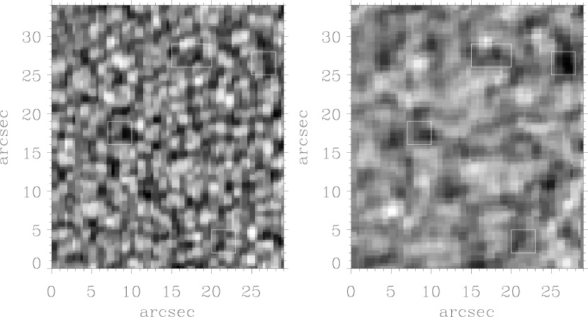
The dataset for this work was obtained on August 10, 2002, in a quiet Sun region close to disk center ($\mu=0.94$). We selected IN regions trying to avoid bright features in the H${\alpha}$ and Ca II K slit-jaw filtergrams supplied by the VTT. Having a few network patches in our fairly large Field-of-View (FOV) is unavoidable, though. In order to point both telescopes to the same region, we benefited from a video link that provided VTT slit-jaw images at THEMIS. First, we pointed both telescopes to an easily identifiable structure, e.g., a sunspot. Then we moved the VTT pointing to a quiet IN region and displaced THEMIS by the same distance. For the data set analyzed here, this method of differential pointing gave an offset of the co-alignment of the two telescopes of 1″. When the offset is corrected it leads to a time lag between the IR and visible data of only 1 minute. We found this offset by shifting the continuum intensity images obtained from the visible and the IR scans (Fig. 1). The optimum shift is chosen as that yielding the minimum difference between the two images. Figure 1 shows the resulting intensities in the IR (left) and the visible (right). Despite the difference in angular resolution, it is clear that both images correspond to the same region. The white boxes point out a set locations on the Sun, and one can easily identify the same structures in the boxes of the two spectral ranges. The spatial resolution for the IR observations is 1″–1$\farcs$2, with a granulation contrast of 1.7%, and it becomes 1$\farcs$5–1$\farcs$7 in the visible, with a contrast of 1.9%. The resolution was estimated as the cutoff of the power spectra of the continuum images shown in Fig. 1. The IR resolution is better due to the use of an active tip-tilt mirror that removes image motion during scanning (Ballesteros et al. 1996). The FOV common to visible and IR observations is of the other of 30″ $\times$ 35″ (Fig. 1).

The data reduction for the IR and visible ranges was very similar: flat field correction, removal of fringes, demodulation to get the Stokes parameters from the measurements, and correction of seeing-induced crosstalk by combining the two beams of each polarimeter. The instrumental polarization (IP) of the VTT was cleared away using a model Mueller matrix for the telescope, which was calibrated with large linear polarizers inserted at the telescope entrance (Collados 2003). THEMIS data do not need this step since it is an IP free telescope. The reduction process renders Stokes $I$, $Q$, $U$ and $V$ profiles in both spectral ranges for each pixel of our FOV. Here we only use intensity and circular polarization. The noise in the polarization measurements was estimated as $3-4\times 10^{-4}~{}I_{\mathrm{c}}$ in the IR data, and $7\times 10^{-4}I_{\mathrm{c}}$ in the visible data ($I_{\mathrm{c}}$ is the continuum intensity). They correspond to the rms fluctuations of the polarization in continuum wavelengths.

3 Data analysis

We select for analysis those IR and visible Stokes $V$ profiles whose peak polarization is larger than three times the noise level. This thresholding separates clear signals from very noisy profiles or pure noise. The pixels with both IR and visible signals above their respective threshold correspond to 30% of the FOV. However, an additional 40% of the pixels present polarization signals only in either the visible or the IR. This study deals with those pixels with signals in both spectral ranges (some 1840).

All selected profiles were classified using a Principal Component Analysis (PCA) algorithm, similar to the one used by Sánchez Almeida & Lites (2000, § 3.2). We classify, simultaneously, the IR and visible Stokes $V$ profiles. All vectors are scaled to the maximum of the blue lobe of the Fe I $\lambda$6302.5 Å Stokes $V$ profile. The PCA classification results in 25 different classes with more than 0.5% of the classified pixels, and 15 classes containing rare profiles (between 0.5% and 0.2%). Figure 2 shows some of the significant classes. We note, firstly, that the IR profiles in class 0 are similar to the most abundant class obtained by Khomenko et al. (2003, Fig. 1). Secondly, class 2 corresponds to network structures in our FOV, and it has characteristic broad IR profiles (also observed in plage regions by Stenflo et al. 1987). Finally, the most conspicuous fact is that some classes (e.g., # 4 and # 8 in Fig. 2) show opposite polarity in the visible and in the IR lines (the lobes have opposite sign).

In order to estimate magnetic field strengths, we performed Milne-Eddington (ME) inversions of the profiles of all individual pixels, as well as the mean profiles among those in each class. We use MILK, a code which is part of the Community Inversion Codes developed by HAO (see Socas-Navarro 2001). Each inversion provides 11 parameters, including the longitudinal component of the magnetic field strength, and the fill factor (fraction of resolution element covered by magnetic fields). (For a description of the procedure and approximations, see, e.g., Skumanich & Lites 1987.) The inversion is separately done for the two pairs of lines, i.e., we carry out two independent inversions per pixel, one for the visible pair and another for the IR pair. In each inversion we use the same atmospheric and magnetic field parameters for the two lines, whereas the ratio of absorption coefficients is fixed according to the expected values. Note that our ME inversion does not fit line asymmetries, although they are clearly present among the observed profiles.

4 Results

The PCA classification indicates that 25% of the pixels with coincident visible and IR signals give visible and IR profiles with opposite polarity. It follows that the visible and IR lines are tracing different magnetic structures in the same resolution element. Some classes have IR profiles with three lobes while the visible profiles have only two (not included in Fig. 2). Actually, the observed Stokes $V$ profiles present a wide variety of asymmetries, in agreement with previous observations (e.g., Sánchez Almeida & Lites 2000; Khomenko et al. 2003).

The ME inversions show that most of the classes have visible Stokes $V$ profiles characteristic of kG fields, while, simultaneously, the IR profiles indicate the presence of sub-kG field strengths. This also happens when we analyze all individual profiles. The result cannot be significantly biased by noise, since the mean profile of a class results from averaging hundreds of profiles and, therefore, bears negligible noise (see Fig. 2). On the other hand, the systematic difference between the IR and the visible is insensitive to the specific technique used to diagnose the field strength. The ratio between the Stokes $V$ extrema of the two visible lines can be used to diagnose the regime of field strength in the atmosphere. A ratio close to 1 indicates kG magnetic fields, whereas a value of some 0.6 is expected for sub-kG fields (see Sect. 5 in Socas-Navarro & Sánchez Almeida 2002). Most of the classes have ratios between 0.9 and 1, which evidences IN magnetic structures in the regime of kG fields. After the inversion of profiles in the various classes, and also from individual profiles, we found a mean magnetic field strength of 1100 G from the visible lines. They fill only 1% of the resolution elements. The mean field strength in the IR is $300$ G, and covers some 2% of the part of FOV studied here.

The ME inversions also show a few classes with weak magnetic fields both in visible and the IR. There are also classes with strong fields in both spectral ranges corresponding to network points in our FOV (class 2 in Fig. 2).

Longitudinal magnetograms measure flux density. One can infer it from ME inversions as the product of the longitudinal component of the field strength times the fill factor. When averaged over the 30% of the FOV that we study, the mean unsigned flux density turns out to be $11$ G in the visible, and $6$ G in the IR. Due to the complexity of the IN magnetic fields, the observed unsigned flux is expected to increase with increasing angular resolution (see, e.g., Sánchez Almeida et al. 2003; Domínguez Cerdeña et al. 2003b). The fact that the IR, with higher resolution, has lower unsigned flux, seems to indicate that this is a true solar effect. Specifically, most of the unsigned magnetic flux of the IN seems to be in the form of kG fields. On the other hand, the signed flux of the region in the visible is $-1.5$ G, while it is less than $0.2$ G in the IR. A similar net flux has been observed before in visible lines (e.g. Lites 2002; Domínguez Cerdeña et al. 2003b). We find it to be co-spatial with very low signed flux in IR lines.

Using magnetic fields from the ME inversion, we have estimated the Probability Density Function (PDF) of finding a given longitudinal magnetic field strength in our IN quiet Sun region. We assume that the visible and the IR polarization signals trace different structures (a reasonable hypothesis, in view of the findings described above). The range of observed field strengths is divided in bins of 50 G. Then, treating visible and IR observations as independent measurements, we assigned each measured longitudinal magnetic field to one of the bins. The probability of finding magnetic field strengths in a given bin (i.e., the PDF) will be proportional to the sum of fill factors of all those measurements in the bin. The result is shown in Fig. 3, the solid line. This PDF has been normalized so that its integral is 0.3, i.e., the fraction of FOV under analysis. In other words, the normalization assumes that the remaining 70% of the surface is field free. Figure 3 includes the PDF for the IR data alone (the dashed line), and for the visible data alone (the dotted line). We also plot the PDF suggested by Socas-Navarro & Sánchez Almeida (2003, the dash-dotted line). We find that 75% of the total flux is concentrated in fields stronger than $500$ G, which, however, occupy only 0.4% of the full FOV.

A final comment is in order. The visible and IR maps that we employ have a time lag of one minute and were coaligned with a finite accuracy (however better than the angular resolution). The lack of strict co-alignment and simultaneity may produce some differences between the visible and the IR spectra, however, they would be of random nature and, consequently, they can hardly explain the observed systematic differences.

5 Conclusions

The (almost) simultaneous visible and IR Stokes $V$ spectra described above have several conspicuous properties. They reveal the coexistence of kG and sub-kG magnetic fields in most of the pixels with polarization signals above the noise (30% of the FOV). The IR lines indicate sub-kG fields whereas visible lines trace kG. This demonstrates the conjecture by Sánchez Almeida & Lites (2000) and Socas-Navarro & Sánchez Almeida (2002, 2003).

At least 25% of pixels with coincident visible and IR signals have one polarity in the visible and the opposite in the IR. This second result offers a direct proof of the existence of two polarities in 1$\farcs$5  resolution elements. They have been inferred from line asymmetries (Sánchez Almeida & Lites 2000), as well as from the skewness of the distribution of line-of-sight magnetic field inclinations in measurements away of the solar disk center (Lites 2002).

The Probability Density Function for the longitudinal magnetic fields, that we infer from ME inversions, has a long tail of kG fields. Some 75% of the observed (unsigned) magnetic flux is in field strength larger than 500 G. This excess of kG flux is in agreement with the PDF suggested by Socas-Navarro & Sánchez Almeida (2003) to reconcile discrepancies between field strengths obtained with different methods (see § 1). We have also found the extended tails in the IR line Fe I $\lambda$15648 Å predicted by such PDF (see classes 0 and 5 in Fig. 2). They carry the information on the strong fields, but are easily misinterpreted due to the large lobes formed by weak fields.

Our observations prove that the use of only visible lines or only IR lines to study the IN fields biases the results. Diagnostics based on simultaneous visible and IR observations offer a viable and reliable alternative.

Figure 1: Continuum intensity images from the IR (left) and the visible spectro-polarimetric scans (right). The squares point out structures which can easily be identified in both images demonstrating the good co-alignment. We scanned along the horizontal direction (solar East-West); the vertical direction is the direction along the spectrograph slit (North-South).

Figure 2: Representative Stokes $V$ profiles from the PCA classification. Mean profiles of Fe I $\lambda$6301.5 Å (left), Fe I $\lambda$6302.5 Å, Fe I $\lambda$15648 Å, and Fe I $\lambda$15652 Å (right) among those in classes 0, 2, 4, 5 and 8 (see the labels on top of the figures, where the percentage of profiles included in each class is also given). Wavelengths are in Å relative to the line center (indicated in each figure as a large plus sign). The small circles represent actual observations whereas the solid lines correspond to ME fits to the observed data.

Figure 3: Probability Density Function (PDF) for observing a longitudinal magnetic field strength $B_{\mathrm{z}}$. The solid line includes both IR and visible data, whereas the distribution of values obtained solely from the IR lines and the visible lines are shown as the dashed and the dotted lines, respectively. The dot-dashed PDF was suggested by Socas-Navarro & Sánchez Almeida (2003) and it is represented for reference.

References

- Ballesteros et al. (1996) Ballesteros, E., Collados, M., Bonet, J. A., Lorenzo, F., Viera, T., Reyes, M., & Rodriguez Hidalgo, I. 1996, A&AS, 115, 353
- Bianda et al. (1999) Bianda, M., Stenflo, J. O., & Solanki, S. K. 1999, A&A, 350, 1060
- Collados (2003) Collados, M. 2003, Proc. SPIE, 4843, 55
- Domínguez Cerdeña et al. (2003a) Domínguez Cerdeña, I., Kneer, F., & Sánchez Almeida, J. 2003a, ApJ, 582, L55
- Domínguez Cerdeña et al. (2003b) Domínguez Cerdeña, I., Sánchez Almeida, J., & Kneer, F. 2003b, A&A, 407, 741
- Faurobert-Scholl et al. (1995) Faurobert-Scholl, M., Feautrier, N., Machefert, F., Petrovay, K., & Spielfiedel, A. 1995, A&A, 298, 289
- Grossmann-Doerth et al. (1996) Grossmann-Doerth, U., Keller, C. U., & Schüssler, M. 1996, A&A, 315, 610
- Khomenko et al. (2003) Khomenko, E. V., Collados, M., Solanki, S. K., Lagg, A., & Trujillo-Bueno, J. 2003, A&A, 408, 1115
- López Ariste et al. (2000) López Ariste, A., Rayrole, J., & Semel, M. 2000, A&AS, 142, 137
- Lin & Rimmele (1999) Lin, H., & Rimmele, T. 1999, ApJ, 514, 448
- Lites (2002) Lites, B. W. 2002, ApJ, 573, 431
- Livingston & Harvey (1975) Livingston, W. C., & Harvey, J. W. 1975, BAAS, 7, 346
- Martínez Pillet et al. (1999) Martínez Pillet, V., et al. 1999, in ASP Conf. Ser., Vol. 183, High Angular Resolution Solar Physics: Theory, Observations, and Techniques, ed. T. Rimmele, K. S. Balasubramaniam, & R. Radick (San Francisco: ASP), 264
- Sánchez Almeida (2003) Sánchez Almeida, J. 2003, in AIP Conf. Proc., Vol. 679, Solar Wind 10, ed. M. Velli, R. Bruno, & F. Malara (New York: American Institute of Physics), 293
- Sánchez Almeida et al. (2003) Sánchez Almeida, J., Emonet, T., & Cattaneo, F. 2003, ApJ, 585, 536
- Sánchez Almeida et al. (1996) Sánchez Almeida, J., Landi Degl’Innocenti, E., Martínez Pillet, V., & Lites, B. W. 1996, ApJ, 466, 537
- Sánchez Almeida & Lites (2000) Sánchez Almeida, J., & Lites, B. W. 2000, ApJ, 532, 1215
- Sigwarth et al. (1999) Sigwarth, M., Balasubramaniam, K. S., Knölker, M., & Schmidt, W. 1999, A&A, 349, 941
- Skumanich & Lites (1987) Skumanich, A., & Lites, B. W. 1987, ApJ, 322, 473
- Smithson (1975) Smithson, R. C. 1975, BAAS, 7, 346
- Socas-Navarro (2001) Socas-Navarro, H. 2001, in ASP Conf. Ser., Vol. 236, Advanced Solar Polarimetry – Theory, Observations, and Instrumentation, ed. M. Sigwarth (San Francisco: ASP), 487
- Socas-Navarro & Sánchez Almeida (2002) Socas-Navarro, H., & Sánchez Almeida, J. 2002, ApJ, 565, 1323
- Socas-Navarro & Sánchez Almeida (2003) Socas-Navarro, H., & Sánchez Almeida, J. 2003, ApJ, 593, 581
- Stenflo et al. (1987) Stenflo, J. O., Solanki, S. K., & Harvey, J. W. 1987, A&A, 173, 167