Massive black hole remnants of the first stars II: optical and X-ray signatures in present-day galactic haloes

Abstract

The first stars forming in minihaloes at redshifts greater than 20 may have been very massive, and could have left behind massive black hole (MBH) remnants. In a previous paper we investigated the hierarchical merging of these MBHs and their associated haloes, using a semi-analytical approach consisting of a hierarchical merger tree algorithm and explicit prescriptions for the dynamics of merged substructure inside a larger host halo following a merger. One of the results was the prediction of a number of MBHs orbiting throughout present-day galactic haloes. In addition, we estimated the mass-accretion rate of these MBHs, assuming that they retained around them a core of material from the original haloes in which they formed. On the basis of these estimates, in this paper we determine the bolometric, optical and X-ray luminosity functions for accreting MBHs, using thin disk and advection dominated accretion flow models. Our predicted MBH X-ray fluxes are then compared with observations of ultra-luminous X-ray sources in galaxies. We find that the slope and normalisation of the predicted X-ray luminosity functions are similar to those observed, suggesting that MBHs could account for some fraction of these sources.

1 Introduction

There is increasing speculation that the first generation of stars in the universe may have been extremely massive, and that some of these objects could have collapsed directly to massive black holes (MBHs) at the end of a brief stellar lifetime. If this is indeed the case, than it has interesting implications for the formation of the super-massive black holes (SMBHs) and unusual X-ray sources observed in the local universe.

Recent semi-analytic [Hutchings  et al. 2002, Fuller & Couchman 2000, Tegmark  et al. 1997] and numerical studies [Bromm, Coppi & Larson 2002, Abel, Bryan & Norman 2000] suggest that the first stars in the universe formed inside dense baryonic cores, as they cooled and collapsed within dark matter haloes at very high redshift. For a standard $\Lambda$CDM cosmology, these minihaloes are estimated to have had masses in the range $M_{min}\sim 10^{5}$–$10^{6}~{}h^{-1}$ ${\rm M}_{\odot}~{}$, and to have collapsed at redshifts $z_{\rm collapse}\sim 20$–$30$ or higher. Since these first star-forming clouds contained essentially no metals, gas cooling would proceed much more slowly in these systems than in present-day molecular clouds. As a result, they may have collapsed smoothly and without fragmentation, producing dense cores much more massive than the proto-stellar cores observed in star-formation regions today. Assuming nuclei within these cores accreted the surrounding material efficiently, the result would be a first generation of protostars with masses as great as $10^{3}$ ${\rm M}_{\odot}~{}$[Bromm, Coppi & Larson 2002, Omukai & Palla 2001].

As yet, nothing definite is known about the subsequent evolution of such objects. However, their large masses would probably result in many of them ending up as MBHs with little intervening mass loss – for systems in this mass range, gravity is so strong that there is no ejection of material from the system in a final supernova bounce [Heger et al. 2002]. This high-redshift population of MBHs is particularly interesting, since it might seed the formation of the SMBHs seen at the centres of galaxies at the present-day.

In a previous paper [Islam, Taylor & Silk 2003, paper I herafter] we used a semi-analytical model of galaxy formation to follow the evolution of MBHs as they merge together hierarchically, along with their associated haloes. The code we used combines a Monte-Carlo algorithm to generate halo merger trees with analytical descriptions for the main dynamical processes – dynamical friction, tidal stripping, and tidal heating – that determine the evolution of merged remnants within a galaxy halo. We introduce seeds into the code by assuming that in each minihalo forming before a redshift $z_{\rm collapse}$, a single MBH forms as the end result of primordial star formation.

For our computations, we considered four different sets of values for the parameters $\nu_{pk}$ and $M_{\bullet,seed}$, which fix the abundance and the mass of the seeds respectively. These values are summarised in table 1. Our choice of a seed MBH mass of 260 ${\rm M}_{\odot}~{}$is motivated by the result of Heger (2002) that massive stars above this mass will not experience a supernova at the end of their lives, but instead will collapse directly to a MBH of essentially the same mass.

Table 1: The mass of seed MBHs, and the height of the peaks in the initial density field in which they formed, for the four models considered. The collapse redshift $z_{\rm collapse}$ is the epoch when peaks of height $\nu_{pk}$ first cross the cooling threshold (see paper I).

Model	$M_{\bullet,seed}$	peak height $\nu_{pk}$	$z_{\rm collapse}$
A	260 ${\rm M}_{\odot}~{}$	3.0	24.6
B	1300 ${\rm M}_{\odot}~{}$	3.0	24.6
C	260 ${\rm M}_{\odot}~{}$	2.5	19.8
D	260 ${\rm M}_{\odot}~{}$	3.5	29.4

In paper I we investigated the abundance of MBHs in present-day galaxies as a result of this process of hierarchical merging and dynamical evolution. This is shown in figure 1.

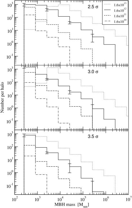
Figure 1: Abundance of all MBHs in the halo for models C, A and D (top to bottom panels) for different final halo masses averaged over 30 trees with error bars corresponding to the standard deviation.

We now look at how this model could be tested observationally in nearby galaxies. As the MBHs orbit they will emit in the optical, UV and X-ray due to accretion of matter in their direct vicinity. This matter can be either the interstellar medium (ISM) of the host, or remnant material of the original satellite that remains bound to the MBH. While optical and UV emissions could in principle arise from a variety of sources and be subject to a range of absorption and distortion mechanisms, X-ray emissions are more uniquely associated with accreting black holes. In addition, hard X-rays are much less subject to absorption. Observations of luminous and ultra-luminous X-ray point sources associated with galactic haloes in the local universe might therefore provide constraints on the existence and abundance of a population of MBHs. Optical and UV observations could be used as a follow up, to confirm the case for detection of a MBH.

In section 2 we outline the accretion scenarios and mechanisms we considered. These include thin disk and advection dominated accretion flows in particular. In section 3 we present the resulting optical and X-ray luminosity functions for MBHs orbiting in present-day haloes. This is then compared with observations of ultraluminous X-ray sources (ULXs) in section 4. We sum up our results and conclude in section 5.

2 Accretion Processes

2.1 Accretion rates

We assume that accretion onto MBHs orbiting in present-day haloes is given by the Bondi-Hoyle mass-accretion rate [Bondi & Hoyle 1944, Bondi 1952]

$$\frac{{\rm~{}d}M}{{\rm~{}d}t}=\pi r_{acc}^{2}\sqrt{v_{\bullet}^{2}+c_{s}^{2}}\rho_{g}$$ (1)

Here $c_{s}$ is the sound speed in the gas and $\rho_{g}$ its density – both far from the MBH. $v_{\bullet}$ is the velocity of the MBH and $r_{acc}$ the accretion radius

$$r_{acc}=\frac{2GM_{\bullet}}{v_{\bullet}^{2}+c_{s}^{2}}$$ (2)

giving an accretion rate

$$\frac{{\rm~{}d}M}{{\rm~{}d}t}=\frac{4\pi G^{2}M_{\bullet}^{2}\rho_{g}}{c_{s}^{3}}(1+\beta_{s}^{2})^{-3/2}$$ (3)

where we have used $\beta_{s}\equiv v_{\bullet}/c_{s}$ [Chisholm, Dodelson & Kolb 2003]. If the MBH accretes adiabatically from a gas of pure hydrogen this is

$$\dot{M} = 8.77\times 10^{-12}\left(\frac{M_{\bullet}}{100M_{\odot}}\right)^{2}\left(\frac{\rho_{g}}{10^{-24}{\rm g~{}cm}^{-3}}\right)$$ (4)

$$\times\left(\frac{c_{s}}{10{\rm~{}km~{}s}^{-1}}\right)^{-3}(1+\beta_{s}^{2})^{-3/2}~{}M_{\odot}{\rm yr}^{-1}$$

If a constant fraction $\eta$ of the accreted mass is radiated away, the bolometric accretion luminosity of the MBH is then

$$L_{bol} = \eta\frac{dM}{dt}c^{2}$$ (5)

$$= \eta~{}5\times 10^{35}\left(\frac{M_{\bullet}}{100M_{\odot}}\right)^{2}\left(\frac{\rho_{g}}{10^{-24}{\rm~{}g~{}cm}^{-3}}\right)$$

$$\times\left(\frac{c_{s}}{10{\rm~{}km~{}s}^{-1}}\right)^{-3}(1+\beta_{s}^{2})^{-3/2}{\rm~{}erg~{}s}^{-1}$$

where $c$ is the speed of light.

In what follows we assume that while the nature of the accretion process is somewhat uncertain, the overall mass-accretion rate is essentially determined by the Bondi-Hoyle formula. We neglect the possibility that the mass-accretion rate is modified e.g. by a non-negligible mass of an accretion disk that may form around the accreting MBHs.

As the MBHs orbit through the host halo they accrete matter from the host ISM. In paper I we have shown that ISM accretion rates are too small to lead to significant accretion signatures even in regions with relatively large amounts of gas, such as the disk or the galactic centre. Much higher rates are possible if MBHs accrete from a residual core of material from the satellite they were originally associated with. Such a core, consisting of gas and possibly stars, could remain bound even if the original satellite has lost all but a few percent of its initial mass. While insignificant for the overall dynamics of the satellite, the amount of baryonic matter contained in this core could still contribute significantly to the accretion onto a MBH that is present at its centre and so boost its accretion luminosity, potentially by orders of magnitude. In this case MBH accretion is independent of local ISM density and of the velocity of the MBH relative to the host halo, as the ‘fuel supply’ for accretion travels with the black hole.

To get a sense of the possible mass-accretion rates allowed by the mechanism, we need to estimate the gas density in the residual baryonic core. We will assume that all the baryons in the original system cool and collapse down to a radius of order $r_{b}\sim 0.1r_{vir}$ (where $r_{vir}$ is the virial radius of the original system), at which point thermal pressure or angular momentum halts the collapse (equivalently we could assume that only a fraction of the baryons collapse, but that $r_{b}$ is slightly smaller). If all baryons are in the form of gas and the baryon fraction in the satellite is cosmological, i.e. $M_{b}=(\Omega_{b}/\Omega_{m})~{}M_{vir}$, then the mean gas density is

$$\rho_{g}=\frac{3M_{b}}{4\pi r_{b}^{3}}=\frac{1}{0.001}~{}\frac{\Omega_{b}}{\Omega_{m}}~{}\frac{3M_{vir}}{4\pi r_{vir}^{3}}\approx 2.39\times 10^{2}\frac{\Omega_{b}}{\Omega_{m}}~{}\frac{M_{vir}}{r_{vir}^{3}}$$ (6)

Substituting this into equation (5) and using $c_{s}\approx 10{\rm~{}km~{}s}^{-1}$ for ISM at $10^{4}$ Kelvin we can determine the mass-accretion rate

$$\dot{m} \approx 6.25\times 10^{-8}\left(\frac{M_{MBH}}{M_{\odot}}\right)\frac{\Omega_{b}}{\Omega_{m}}\left(\frac{M_{vir}}{10^{5}M_{\odot}}\right)$$ (7)

$$\times\left(\frac{r_{vir}}{{\rm kpc}}\right)^{-3}\left(\frac{c_{s}}{10{\rm~{}km~{}s^{-1}}}\right)^{-3}$$

and thus the luminosity. Here $\dot{m}$ is the mass-accretion rate in units of the Eddington accretion rate

$$\dot{m}\equiv\frac{\dot{M}c^{2}}{L_{E}}=1.53\left(\frac{\dot{M}}{10^{17}{\rm g~{}s}^{-1}}\right)\left(\frac{M_{\bullet}}{M_{\odot}}\right)^{-1}$$ (8)

2.2 Accretion mechanisms

As material gets accreted onto a Black hole, a fraction of its gravitational potential energy released as radiation. The amount and spectrum of energy released in such a way depends on the accretion model, that is a prescription for the physical processes that facilitate the dissipation of energy as material moves towards the accreting MBH. We consider two of these.

2.2.1 Thin disk accretion

Shakura & Sunyaev (1973) proposed a model in which black holes (BHs) accrete from a geometrically thin but optically thick accretion disk, which is considered to achieve the highest radiative efficiencies, typically with $\eta_{td}\sim 0.1$. Because the disk is optically thick, radiation is emitted locally with a thermal spectrum and black body temperature

$$T(r)=\left(\frac{3GM_{\bullet}\dot{M}}{8\pi r^{3}\sigma}\right)^{1/4}$$ (9)

where $\dot{M}$ and $r$ are the mass-accretion rate and radial distance from the MBH respectively. We can convert these into dimensionless quantities and express the accretion rate in units of the Eddington accretion rate equation (cf. equation 8) and the radial distance from the MBH in units of the MBH Schwarzschild radius, $r_{\bullet}$

$$\tilde{r}\equiv\frac{r}{r_{\bullet}}=\frac{r~{}c^{2}}{2~{}G~{}M_{\bullet}}=0.339\left(\frac{r}{{\rm km}}\right)\left(\frac{M_{\bullet}}{M_{\odot}}\right)^{-1}$$ (10)

The corresponding spectrum integrated over the whole disk is given by [Frank, King, & Raine 1985]

$$\frac{{\rm~{}d}L_{\nu}}{{\rm~{}d}\nu}=A_{0}\frac{h\nu^{3}}{c^{2}}\int^{r_{td}}_{r_{lso}}\frac{\tilde{r}{\rm d}\tilde{r}}{e^{h\nu/kT(\tilde{r})}-1}$$ (11)

where $r_{lso}=3~{}r_{\bullet}$ is the last stable orbit radius of the MBH and $A_{0}=4~{}\pi$ is the area of a spherical shell at unit distance from the MBH. However, in what follows we treat $A_{0}$ more generally as a normalisation constant. All our computations were carried out with $r_{td}=1000r_{\bullet}$ and $A_{0}$ was consequently renormalised by setting $\int({\rm~{}d}L_{\nu}/{\rm~{}d}\nu){\rm d}\nu=L_{bol}$. The resulting spectra are shown in the panels on the right in figure 2.

In general the accretion flow near the BH may become optically thin and absorption of photons becomes less important than scattering, which results in an increase of the mean energy of the photons radiated away. The emergent flux is thus non-thermal and has a higher temperature. Consequently in the inner parts of the disk near the MBH, equations 9 and 11 are not strictly valid anymore. Another prescription to account for the higher frequency photons is needed.

This high-frequency emission also has important observational consequences. MBHs are only clearly identified as BHs via an X-ray signature. However, from equation 9 the peak frequency of the photons from a standard thin disk scales as $\nu_{max}\propto T(r_{lso})\propto M_{\bullet}^{1/4}$. For the MBHs any resultant flux in the X-ray range is only significant at energies below about 1 keV. A standard thin disk alone would therefore not provide the X-ray flux by which to identify MBHs.

One could tackle this problem phenomenologically by adding a power-law spectrum extending into the X-ray range. A power law X-ray spectrum is well established for active galactic nuclei (AGN), which are driven by SMBHs, and is also found in recent observations of ultra-luminous X-ray sources in nearby galaxies, which could well be accreting MBHs [Colbert & Mushotzky 1999, Wang 2002]. However, instead we consider a different model that has recently been developed particularly with a view to explaining the emission spectra from accreting SMBH in low-luminosity AGN. This is an advection dominated accretion flow.

2.2.2 Advection dominated accretion flows (ADAFs)

In the ADAF model, once the accretion rate drops below some critical rate $\dot{m}_{crit}$, which we define below, accretion switches to an ‘advection dominated accretion flow’ (ADAF) [Ichimaru 1977, Rees et al. 1982, Narayan & Yi 1994, Manmoto, Mineshige & Kusunose 1997]. Because of the low accretion rates the density of the accreted gas is low, too. The gas, not being able to cool, efficiently stores thermal energy instead of radiating it away and carries it into the BH. On the other hand, because the accretion flow is optically thin the spectrum of the emergent radiation is modified by scattering processes. The main processes are synchrotron emission, bremsstrahlung and comptonisation. For more details the reader is referred to the review by Narayan, Mahadevan & Quataert (1998) and references therein.

The spectrum emitted from a BH accreting in this way depends on a range of parameters such as the mass-accretion rate , the viscosity parameter and the relative contribution of magnetic fields. Typically the spectrum has to be determined numerically, but can be approximated by analytic scaling relations [Mahadevan 1997]. Using these, the total radiative efficiency for an ADAF, $\eta_{adaf}$ can be expressed in terms of that of a thin disk, $\eta_{td}$ as

$$\eta_{adaf}=0.2\eta_{td}\left(\frac{\dot{m}}{\alpha^{2}}\right)g(\theta_{e})$$ (12)

for a typical set of parameters as given in Mahadevan (1997). Here $\dot{m}$ is the mass-accretion rate in terms of the Eddington accretion rate, $\alpha$ is the viscosity parameter ($\alpha\sim 0.1$ to $0.5$), $\theta_{e}=k_{B}~{}T_{e}/(m_{e}~{}c^{2})$ is the electron kinetic energy in units of their rest mass energy. $g(\theta_{e})\approx 11.5(T_{e}/10^{9}{\rm K})^{-1.3}$ is a measure of whether electrons in the flow move at relativistic speeds or not. Typically $g\sim 1$ to $10$ for electron temperatures $2\times 10^{9}<T_{e}<10^{10}$ K. We can determine an equilibrium electron temperature which is approximately

$$\left(\frac{T_{e}}{10^{9}{\rm K}}\right)\approx\left(\frac{\alpha}{0.3}\right)^{-0.06}\left(\frac{r_{min}}{3}\right)^{0.1}~{}M_{\bullet}^{0.06}~{}\dot{m}^{-0.04}$$ (13)

Generally the effect of ADAFs is to reduce the overall radiative efficiency compared to that from thin disk accretion, although individual regions of the accompanying spectrum, especially the X-ray band, tend to be much stronger than for a thin disk.

As mentioned above the thin disk and ADAF regime can be delineated by the critical mass accretion rate $\dot{m}_{crit}$ which is given by

$$\dot{m}_{crit}\geq 0.28\alpha^{2}$$ (14)

For rates above $\dot{m}_{crit}$ the ADAF mechanism breaks down and in this regime we will work with the thin disk model. For low values of $\alpha\leq 0.1$ accretion may switch to a ‘convection dominated accretion flow’ (CDAF) [Ball, Narayan & Quataert 2001], which is characterised by much stronger suppression of mass accretion. We will neglect this possibility here as we work with $\alpha=0.3$ in the computation of spectra and luminosity functions for our model. This is also the fiducial value used in the work of Mahadevan (1997). We will briefly consider changes in $\alpha$ below.

In paper I we have seen that MBHs do not accrete at more than 1/10 of the Eddington rate with most accreting at less than 1/100. Thus the ADAF model can be applied to most MBHs we are dealing with.

The three dominant contributions to the continuum spectrum of an ADAF are those from synchrotron and bremsstrahlung emission as well as comptonisation, which can all be separately approximated by scaling laws [Mahadevan 1997]. In the radio-submillimeter range synchrotron emission dominates and the luminosity (per unit frequency) scales as

$$\frac{{\rm~{}d}L_{sync}}{{\rm~{}d}\nu} \simeq 3.51\times 10^{13}~{}\left(\frac{\alpha}{0.3}\right)^{-4/5}\left(\frac{T_{e}}{10^{9}~{}{\rm K}}\right)^{2/5}$$ (15)

$$\times\left(\frac{M_{\bullet}}{M_{\odot}}\right)^{6/5}~{}\dot{m}^{6/5}~{}\nu^{2/5}{\rm~{}erg~{}s}^{-1}~{}{\rm Hz}^{-1}$$

up to a peak frequency $\nu_{p}$ given by

$$\nu_{p} = 1.71\times 10^{17}\left(\frac{\alpha}{0.3}\right)^{-1/2}\left(\frac{T_{e}}{10^{9}{\rm K}}\right)^{2}\left(\frac{M_{\bullet}}{M_{\odot}}\right)^{-1/2}$$ (16)

$$\times\left(\frac{r_{min}}{3}\right)^{-5/4}~{}\dot{m}^{3/4}{\rm Hz}$$

Photons from synchrotron emission can get comptonised, which raises their energy up to a limit given by the electron temperature $k_{B}~{}T_{e}$. Since most synchrotron photons are emitted at $\nu=\nu_{p}$ we can make the simplifying assumption that this is the initial frequency for all photons to be comptonised. The comptonisation spectrum is then simply

$$\frac{{\rm~{}d}L_{compt}}{{\rm~{}d}\nu}\simeq\frac{{\rm~{}d}L_{sync}}{{\rm~{}d}\nu}(\nu_{p})\left(\frac{\nu}{\nu_{p}}\right)^{-\alpha_{c}}$$ (17)

where the power law index is primarily a function of electron temperature and mass-accretion rate

$$\alpha_{c}\equiv-\frac{{~{}\rm ln}\left[23.87\dot{m}\left(\frac{\alpha}{0.3}\right)^{-1}\left(\frac{r_{min}}{3}\right)^{-1/2}\right]}{{~{}\rm ln}\left[1+4~{}\theta_{e}+16\theta_{e}^{2}\right]}$$ (18)

There is a constant contribution from bremsstrahlung emission that also tails off exponentially at the maximum frequency implied by the electron temperature. Bremsstrahlung only becomes prominent in the UV/soft X-ray range if $\alpha_{c}>1$, such that power from Compton emission effectively decreases with increasing frequency

$$\frac{{\rm~{}d}L_{brems}}{{\rm~{}d}\nu} \simeq 1.02\times 10^{17}\left(\frac{\alpha}{0.3}\right)^{-2}{~{}\rm ln}\left[\frac{r_{max}}{r_{min}}\right]$$ (19)

$$\times F(\theta_{e})\left(\frac{T_{e}}{10^{9}{\rm K}}\right)^{-1}e^{-h\nu/k_{\small B}T_{e}}$$

$$\times\left(\frac{M_{\bullet}}{M_{\odot}}\right)\dot{m}^{2}{\rm erg~{}s^{-1}~{}Hz^{-1}}$$

If $\theta_{e}<1$, $F(\theta)$ takes the form

$$F(\theta_{e}) = 4\left(\frac{2\theta_{e}}{\pi^{3}}\right)^{1/2}(1+1.78\theta_{e}^{1.34})$$ (20)

$$+1.73\theta_{e}^{3/2}(1+1.1\theta_{e}+\theta_{e}^{2}-1.25\theta_{e}^{5/2})$$

whereas for the case $\theta_{e}>1$,

$$F(\theta_{e}) = \left(\frac{9\theta_{e}}{2\pi}\right)[{~{}\rm ln}(1.123\theta_{e}+0.48)+1.5]$$ (21)

$$+2.3\theta_{e}({~{}\rm ln}1.123\theta_{e}+1.28)$$

The resulting spectrum is shown in the left panels of figure 2 for a range of MBH masses and accretion rates ranging from $\dot{m}=\dot{m}_{crit}$ to $\dot{m}=0.03~{}\dot{m}_{crit}$, where $\dot{m}_{crit}=0.0252$ for $\alpha=0.3$ which we use for all our computations.

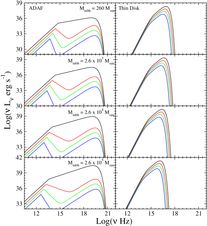
Figure 2: Emission spectra from ADAF (left) and thin disk (right) accreting MBHs in the mass range between $2.6\times 10^{2}$ to $2.6\times 10^{5}$ ${\rm M}_{\odot}~{}$. In each panel the curves from top to bottom correspond to mass-accretion rates $\dot{m}=\{1,0.3,0.1,0.03\}~{}m_{crit}$, where $m_{crit}=0.0252$ for $\alpha=0.3$.

We see that only ADAF accreting MBHs display significant X-ray emission. It is therefore mainly MBHs that could be identified as such by their X-ray signature. Conversely, while optical and UV observations may be used as follow-ups, the sources that are most luminous in this range are accreting from a thin disk and so will not have any associated strong X-ray emission.

X-ray hardness ratios
For our predictions we have computed the X-ray emissions for the energy range between $0.5<h~{}\nu<2.0$ keV and $2.0<h~{}\nu<10.0$ keV , which we call the soft and hard X-ray bands respectively. Both bands lie in the Bremsstrahlung part of the ADAF spectrum where ${\rm~{}d}L/{\rm~{}d}\nu=1$, i.e. the photon counts from both bands are the same; their hardness ratio is equal to 1. Unfortunately, observations from X-ray binaries (XRBs) can yield similar values, so it will not be easy to distinguish between MBHs and XRBs on the basis of this alone. The combined thin disk + ADAF model that we used, means that we can also have sources with large soft X-ray luminosities and very small hardness ratios. This is the case particularly for seed MBHs for which thin disk accretion reaches furthest into the soft X-ray regime, and there actually dominates over the respective ADAF contribution (cf. figure 2). In section 3.2 we see that this leads to a distinctive ‘bump’ in the soft band luminosity function. These sources should be identifiable by their very low hardness ratio.

3 Predicted Luminosity Functions

Using the spectral models outlined above we have computed optical and X-ray luminosities of accreting MBHs in present-day haloes. For comparison we show in figure 3 the bolometric luminosity functions, obtained in paper I.

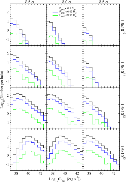
Figure 3: Bolometric luminosity of MBHs accreting from baryonic cores for models C, A and D (left to right panels). Shown are the sources whose line of sight falls within some projected distance from the host centre.

3.1 Optical emission

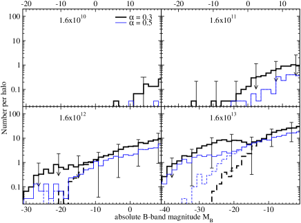
Figure 4: Average B-band luminosity functions for MBHs in haloes of various masses, for two different values of $\alpha$ (two sets of lines). The dashed lines show the contribution from ADAF accretion. Thin disk emission dominates at large luminosities.

For the MBH masses we are considering here, the optical region lies within the Rayleigh-Jeans part of the extended black body spectrum that characterises the corresponding thin disk emission. In this part, $k_{B}T(r_{td})\ll h\nu\ll k_{B}T(r_{lso})$ where the spectrum can be approximated by a power law

$$\frac{{\rm~{}d}L}{{\rm~{}d}\nu}=A_{1}\left(\frac{\nu}{{\rm Hz}}\right)^{1/3}$$ (22)

and the constant $A_{1}$ depends on the MBH mass and accretion rate as

$$A_{1} = 2.57~{}A_{0}~{}h^{-5/3}~{}k_{B}^{8/3}~{}c^{-2}~{}T(r_{lso})^{8/3}$$

$$\approx 1.64\times 10^{11}~{}A_{0}~{}\dot{m}^{2/3}~{}M_{\bullet}^{4/3}~{}{\rm erg~{}s^{-1}~{}Hz^{-1}}$$

In the ADAF regime it is primarily synchrotron emission and comptonisation that contribute to the emission in the optical/UV range, with the corresponding scalings given in equations 15 and 17.

Figure 4 shows the B-band luminosity function. The dashed line represents the contribution from ADAF emission with the rest, primarily at large luminosities, coming from thin disk emission. Apart from our fiducial value for the viscosity parameter, $\alpha=0.3$ (thick lines), we have also given results for $\alpha=0.5$ (thin lines). While the results for ADAF emission are typically not too sensitive to changes in ADAF parameters, results are affected more strongly by changes in $\alpha$, but only through its direct impact on the value of $\dot{m}_{crit}$ (cf. equation 14). As a result the most important effect of increasing $\alpha$ is to extend the number of ADAF emitting sources to larger luminosities. Since a thin disk radiates more efficiently than an ADAF this results in a lower abundance of sources at very large magnitudes in the optical range. For smaller values of $\alpha$ we get a correspondingly larger number of thin disk accreting sources. However, we found that for a value of $\alpha=0.1$, for instance, the resulting luminosity function in the B-band displays a significant ‘dip’ which is also present to some degree for $\alpha=0.3$ in the case of the most massive $1.6\times 10^{13}$ ${\rm M}_{\odot}~{}$halo in figure 4. We will deal with the results for the X-ray range in the next section, but note at this point that a higher (lower) value of $\alpha$ would result in a larger (lower) abundance of sources in the X-ray regime, emission in which is mainly produced in ADAFs.

In figure 5 we show the B and V band luminosity function of MBHs within some projected distance from the host centre normal to the line of sight. Here we have included all MBHs within the respective host virial radius along the lines of sight passing within some projected distance from the centre. We will subsequently refer to this as the projected luminosity function. The projected luminosity function can more easily be compared with observations, which typically refer to sources within galaxies. In each case the function is plotted for MBHs sources within $R_{proj}=0.1,0.03,0.01~{}R_{vir}$ from the host centre, where the latter corresponds roughly to the outer radial extent of the galaxies in the haloes. Across all halo masses we find that a fraction of about 30, 9 and 0.9 % respectively of all halo MBHs are located within the projected distances listed above. Since there is no discernible difference in the relative distribution of MBH masses at different radii (paper I), this means that for any one MBH in a given mass, accretion rate or luminosity range and within $R_{proj}=0.1R_{vir}$, there are about two more in the halo. We have marked with bold black arrows the luminosity range below which ADAF emission dominates.

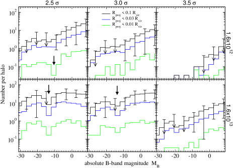
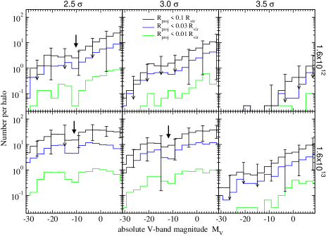
Figure 5: Optical luminosity function for MBHs accreting from baryonic cores within various projected distances from the host centre. Results are shown for models C, A and D (three sets of panels, left to right) in the B and V-band (left-hand and right-hand figures). The bold arrows delineate where luminosities are dominated by thin disk emission and ADAF emission respectively.

It is important to note that these luminosity functions only provide an upper limit on what could actually be detected. We have here neglected the effect of absorption which is expected to significantly reduce the flux of optical and UV photons due to dust and neutral hydrogen along the line of sight. The latter affects particularly the light from sources whose line of sight passes closely to the galactic centre, such as those with $R_{proj}<0.01R_{vir}$ and located on the far side of the halo. We would expect this effect to be less important in gas-poor ellipticals.

Even if absorption is accounted for, the large luminosity of the accreting MBHs by itself may not be sufficient to identify them as such. As they appear as point sources, they could also be XRBs or background AGN. For the largest accretion rates, $\dot{m}\sim 0.1$ (paper I), at which MBHs accrete from a thin disk in our model, it is possible that emission occurs in the form of (mini) jets which may be observable even though the optical and UV output from across the accretion disk may not.

3.2 X-rays

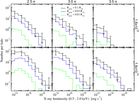
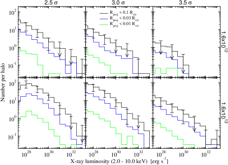
Figure 6: X-ray luminosity function of MBHs with (line-of-sight within) various projected distances from the host centre (see also text). Results are shown for models C, A and D (three sets of panels, left to right) and X-rays in the energy range from 0.5 - 2.0 keV (left-hand figure) and 2.0 - 10.0 keV (right-hand figure).

In our model X-rays are primarily emitted by ADAF accreting MBHs. Emission in the X-ray range is dominated by comptonisation or bremsstrahlung depending on the Compton spectral power law index, $\alpha_{c}$ (eq. 18). The two contributions are determined by the scaling relations equations 17 and 19. In figure 6 we present the projected X-ray luminosity function, both in the 0.5 - 2.0 keV and 2.0 - 10.0 keV energy range. Again we have ignored the issue of absorption here, which can be important primarily for the softer 0.5 - 2.0 keV X-ray band.

X-ray emissions are the primary signature to look for in observations, while optical and UV detections are probably useful only for follow-up, due to the range of potential sources and the problem of absorption. Another secondary diagnostic would be to see whether any correlations exist between different parts of the emitted spectrum. However, this would be extremely dependent on the accretion model. For instance, in the ADAF model that we used, the shape of the spectrum near the exponential cut-off in the X-ray regime and in the radio/submillimeter range is essentially unaffected by the mass and accretion rate of the MBH (cf. figure 2). If a MBH accretes via an ADAF we would therefore expect a correlation of the radio and X-ray luminosities.

4 Comparison with Observations

We now compare our predictions with observations. As we have already noted, X-ray emissions will be the most important trace to look for. We will therefore confine our comparison to X-ray observational data only and further more to sources which have been identified as belonging to a galaxy.

In our predictions we have generally not taken into account absorption of MBH emission either in the originating galaxy as well as ours. To minimise the former one would want to look for sources in external galaxies that we see face-on. This is especially important for gas-rich spirals. To account for the extinction from the IGM and the Milky-Way’s ISM all-sky extinction maps can be used [Schlegel, Finkbeiner & Davis 1998]. These allow a determination of the average hydrogen column density between us and the target galaxy.

4.1 Observations of ultra-luminous X-ray sources (ULXs)

For the baryonic core densities and accretion mechanisms considered above, our model predicts the presence of ultra-luminous X-ray sources (ULXs) in galaxies and their haloes. By ULX we refer to any compact X-ray source with $L_{X}\mathrel{\hbox{\hbox to0.0pt{\hbox{\lower 4.0pt\hbox{$\sim$}}\hss}\hbox{$>$}}}10^{38}{\rm erg~{}s}^{-1}$. This cutoff is interesting because it corresponds roughly to the Eddington limit for isotropic accretion onto stellar-mass black holes. Early observations revealed that some galaxies contain these very bright sources outside their nucleus [Fabbiano 1989]. Subsequently, a number of other studies discovered ULXs in data from the ROSAT and ASCA satellite missions [Colbert & Mushotzky 1999, Makishima  et al. 2000, Roberts & Warwick 2000, Colbert & Ptak 2002]. With the advent of the Chandra and XMM satellite missions, the number of ULX detections has soared. The superior resolution and sensitivity of these satellites has greatly increased the distance at which ULXs can be detected, and thus the number of galaxies in which their properties can be studied.

While ‘normal’ stellar remnants may easily account for the fainter ULXs, sources which emit more than a few times $10^{39}{\rm erg~{}s}^{-1}$ require black holes more massive than those produced by conventional stellar populations, assuming the emission is Eddington limited and occurs isotropically. If ULXs do not emit isotropically, however, but produce beamed emission that happens to be aligned with the line-of-sight, then stellar mass BHs can be the source [King  et al. 2001, Zezas & Fabbiano 2002]. A departure from isotropy implies that the Eddington luminosity is no longer a limiting factor, either, as radiation pressure need not act along the same axis as the accretion flow. High mass X-ray binaries (HMXRBs) have been suggested as candidates for anisotropic ULXs. Within galaxies, ULXs appear to be found predominantly in star-forming regions [Kilgard  et al. 2002, Zezas & Fabbiano 2002], i.e. they seem to be associated with starburst galaxies or the spiral arms of disk galaxies. For a number of these galaxies it was found that the ratios of ULX number to massive star formation rates are similar [Smith & Wilson 2003]. Thus many ULXs may be young HMXRBs, which would naturally be found in or close to star-forming regions.

There is some evidence, however, to suggest that not all ULXs fall into this category. Multi-colour disk (MCD) fits to ULX spectra indicate that the maximum colour temperature associated with some sources is significantly lower than would be expected for a stellar mass BH system. If the maximum temperature arises from emission close to the inner radius of the accretion disk, and we assume this to be the BH’s last stable orbit, a lower temperature implies a larger stable orbit and thus a more massive BH [Wang 2002]. Furthermore, ULXs have been detected in some gas-poor ellipticals [Jeltema & Canizares 2003], and Colbert & Ptak (2002) find that the number of ULXs per galaxy is actually higher for ellipticals than for non-ellipticals. Thus the connection between ULXs and star formation established for spiral galaxies may not be universally valid. It seems interesting, therefore, to consider alternative explanations for these sources, such as isotropically emitting MBHs.

If seed MBHs do account for some of the observed ULXs, there are a few remaining puzzles to work out. It is not clear whether our model should predict more ULXs around spirals or ellipticals, and the morphological information in the model is probably too crude to test this definitively. Since ellipticals are generally older systems, however, it is not implausible that they would have a large number of ancient satellites in orbit around them. A number of ULXs seem to be located in globular clusters [Jeltema & Canizares 2003], suggesting binaries are the corresponding ULX sources. In the context of our model, however, some of these globular clusters might be precisely the baryonic cores we have considered previously.

Ultimately, detailed spectral information should allow us to distinguish between binaries and MBHs as ULX candidates. Reasonable spectral information is available for some systems, although fits to such data still assume model spectra which should be verified independently. For the more distant sources, the detected count rates are so low that spectral fits cannot be carried out. Instead a hardness ratio, the ratio of the number counts in a soft and a neighbouring hard X-ray band, can be used as a crude diagnostic. Uncertainties in the correction for absorption in soft X-ray bands complicate the interpretation of these results, however. Here we will avoid these complications, using spectral information only to the extent that it allows X-ray band luminosities to be derived from raw photon counts. We will not use spectral fits to make any inference about the ULX source object.

In summary, while binaries may explain the majority of ULXs, especially in star-forming galaxies, MBHs are not ruled out as a possible source of some of these objects. In what follows, we will show how the free-floating MBHs predicted by our model could account some fraction of all ULXs. The exact fraction is highly model dependent; for the parameters assumed above, we will show it can be considerable.

4.2 Comparing Luminosity Functions

Table 2 gives a summary of the observations of point sources in individual galaxies that we are considering. Their inferred masses roughly place them in a category with the $1.6\times 10^{12}$ ${\rm M}_{\odot}~{}$halo in our model. Observed sources are considered roughly within the light radius of the galaxy. Where observations do cover regions significantly outside this radius it is typically an area to one side of a galaxy that happens to be still covered by the detector. Interestingly, a number of ULXs are detected in this area as well. Estimates of the expected number of background objects, such as AGN, supernovae (SN), etc. show that they can account for most of the ULXs observed outside the light radius, although the error margins are large. A number of sources outside the bulge have projected locations that appear to be in the disk. In this case background sources cannot account for the relatively large number of sources that seem to lie in the disk. It is assumed on this basis that these sources are actually located in the disk, where their number can be explained more naturally. For sources with apparent locations in the disk as well as outside the light radius our model offers the alternative explanation that some of these sources could also be located throughout the halo but inside a column along the line of sight that projects onto the disk.

Table 2: Summary of X-ray observations. The first four galaxies are spirals; NGC 720 is an elliptical. All observations were carried out with the ACIS instrument on Chandra, except for the observation of M31 which was observed with Chandra’s HRC instrument.

Galaxy	Energy range	Region surveyed	# ULXs	Reference
M31 (S)	0.1 - 10 keV	$R_{proj}<1.13{\rm kpc}$	3	[Kaaret 2002]
M81 (S)	0.3 - 8 keV	$R_{proj}>D_{25}$	2	[Swartz  et al. 2003]
		disk	10
		bulge	5
	0.2 - 8 keV	disk ($R_{proj}\mathrel{\hbox{\hbox to0.0pt{\hbox{\lower 4.0pt\hbox{$\sim$}}\hss}\hbox{$<$}}}8.5{\rm kpc}$)	5	[Tennant  et al. 2001]
		bulge	3
NGC 6964 (S)	0.5 - 5 keV	$R_{proj}\mathrel{\hbox{\hbox to0.0pt{\hbox{\lower 4.0pt\hbox{$\sim$}}\hss}\hbox{$<$}}}13{\rm kpc}$	15	[Holt  et al. 2003]
NGC 1068 (S)	0.4 - 5 keV	$R_{proj}<D_{25}$	40	[Smith & Wilson 2003]
NGC 720 (E)	0.3 - 10 keV	$R_{proj}\mathrel{\hbox{\hbox to0.0pt{\hbox{\lower 4.0pt\hbox{$\sim$}}\hss}\hbox{$<$}}}25{\rm kpc}$	41	[Jeltema & Canizares 2003]

Given the uncertainties and free parameters in our model, we cannot place a strong constraint on MBHs from ULX observations alone. Nonetheless, it is interesting to make a quantitative comparison between the observations and our model predictions, particularly since the predictions scale in a straightforward way as the number or mass of the seeds, or the density of the baryonic cores, varies. Since our models often predict one or fewer luminous sources per system, the comparison with observations will be statistical; this is all the more true since we predict a large halo-to-halo scatter in the number of MBHs, and thus in the X-ray luminosity functions. In general, even if MBHs accounted for all ULXs, we would expect a variation in the luminosity functions of individual galaxies that was comparable to the halo-to-halo scatter in our results.

We first look at how our results compare with observations of sources in individual galaxies. Figure 7 shows the cumulative X-ray luminosity function from observations and those that we predict for a $1.6\times 10^{12}$ ${\rm M}_{\odot}~{}$halo, which would be expected to host galaxies of the mass we are comparing with. For our predictions we have chosen two different X-ray bands as shown in the figure to match those from the observations more closely. Our predictions are consistent with the data from the individual galaxies if we only consider the ADAF emissions. Inclusion of the thin disk component leads to a much flatter slope and an over prediction of sources at the high luminosity end. The flat slope essentially bridges the gap in the differential luminosity function between ADAF accreting MBHs and a small number of MBHs accreting from a thin disk as shown in figure 6. Whether the thin disk is included or not, MBHs cannot account for the large number of sources at low luminosities, which is not a problem as we expect XRBs to certainly dominate this regime.

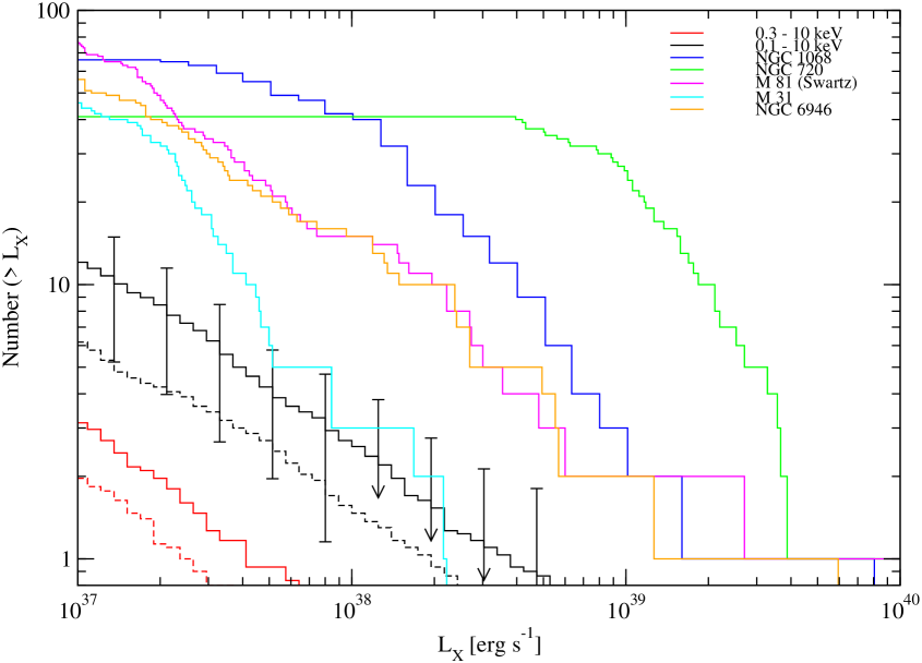
Figure 7: Cumulative X-ray luminosity functions for five galaxies observed by Chandra (see text), compared with our model predictions. The solid black line with error bars shows our predicted cumulative luminosity functions for model C in the 0.1-10 keV band, while the dashed line immediately below it shows the same for model A. The two lines below this are for models C and A in the 0.3-10 keV band. In each case only those sources with projected radii $<30$ kpc from the galactic centre are included.

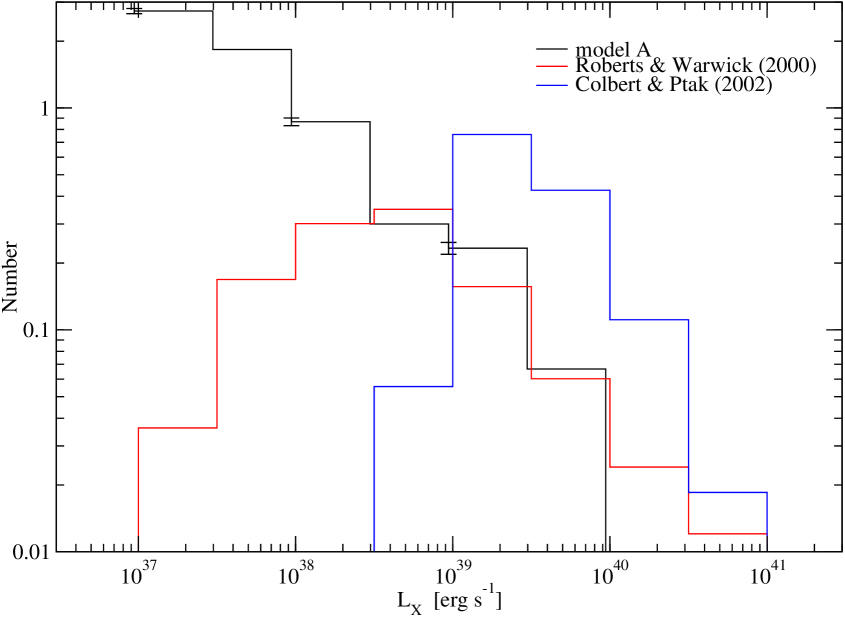
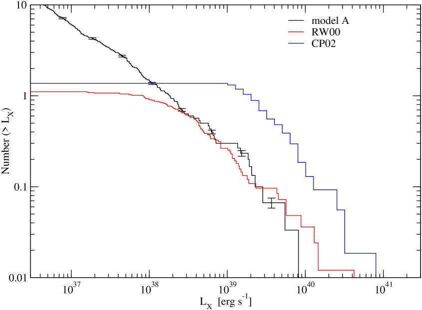
Figure 8: Differential (top panel) and cumulative (bottom) luminosity functions for predictions from model A ($1.6\times 10^{12}$${\rm M}_{\odot}~{}$halo) and observations. Note in particular the similar slope for luminosities larger than $10^{38}{\rm erg~{}s}^{-1}$. Only sources at radial distances larger than $R>0.01~{}R_{vir}\approx 3$ kpc were considered. The predicted values only account for sources at projected distances less than $R_{proj}<0.1~{}R_{vir}\approx 30$ kpc.

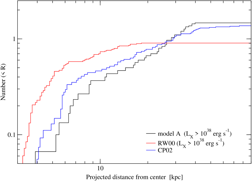
Figure 9: Projected radial distribution of sources with $L_{X}>10^{38}{\rm erg~{}s}^{-1}$, as predicted from model A ($1.6\times 10^{12}$${\rm M}_{\odot}~{}$halo), compared with observations. Only sources at radial distances larger than $R>0.01~{}R_{vir}\approx 3$ kpc were considered. The predicted values only account for sources at projected distances less than $R_{proj}<0.1~{}R_{vir}\approx 30$ kpc.

For luminosities larger than $L_{X}\sim 10^{38}{\rm erg~{}s}^{-1}$, the predicted average numbers of objects are near or below 1 and we have to compare with observations of a statistical sample of galaxies. The two data sets we use for this are that of Roberts &Warwick (2000, hereafter RW00) and Colbert & Ptak (2002, hereafter CP02) . Both sets of observations have been obtained using the ROSAT High Resolution Imager (HRI) instrument. In comparing with these observations, we quote the error on the mean (and not the standard deviation of the halo-to-halo scatter) for our predictions. The two sets of observations vary fundamentally in that CP02 only consider galaxies that do contain ULXs. They find a total of 87 sources in 54 galaxies of which 15 are ellipticals. They note that in their sample the number of ULXs per galaxy is larger for ellipticals, which account for a total of 37 ULXs. This corresponds to 2.3 ULXs per galaxy for ellipticals compared to 1.3 per galaxy in the case of non-ellipticals. As the CP02 sample only counts galaxies that contain ULXs the derived luminosity and spatial distributions will have a systematic offset towards higher abundances.

The differential and cumulative luminosity functions are shown in figure 8, for the observations and for our expected source population for the galaxy-sized $1.6\times 10^{12}$${\rm M}_{\odot}~{}$halo in model A. We note that the luminosity bands used in the two data sets are different; while RW00 quote results for the ROSAT 0.1 - 2.4 keV band, CP02 give their data for the 2.0 - 10.0 keV range. To match these we have slightly changed our soft bands from the one used above (0.5 - 2.0 keV). Furthermore, we have only taken into account sources at radial distances less than 10 % of the halo virial radius, which corresponds to about $R<30$ kpc for this halo. This is also of the order of the limiting radii below which sources in the CP02 sample are considered as belonging to a galaxy.

Between $3\times 10^{38}$ and $10^{40}{\rm erg~{}s}^{-1}$, our predictions in the hard band and the soft band without the thin disk contribution match the slope and normalisation of RW00. A power-law best fit yields a logarithmic slope of $-0.83\pm 0.03$,$-0.78\pm 0.01$ and $-1.08\pm 0.01$ for our prediction, RW00 and CP02 respectively. For lower luminosities the down-turn (tailing off) in the differential and cumulative distribution of the RW00 data is probably due to incompleteness. Even if no MBHs were present there would still be enough XRBs to match or exceed the number of objects at lower energies. Including the thin disk in the soft band leads to the black curve on the right, which is ruled out even by the CP02 data which, as we mentioned above, is biased towards higher abundances.

Aside from the uncertainty in our model parameters, there are also several physical processes that may reduce the luminosity of the brightest sources. The relatively large accretion rates in MBHs accreting from thin disks could exhaust the baryonic core, if the latter was not large enough to start with. Past merger activity of MBH hosts might also have triggered periods of mini-quasar activity that has lead to a faster depletion of gas in the baryonic core. Alternately, if the accretion rates were slightly lower than assumed, by a factor 5 or so, then most systems would fall below the critical accretion threshold (equation 14), and would accrete in the ADAF mode. Abandoning the thin disk contribution would also remove the brightest sources in the B and V band luminosity functions.

In figure 9 we show the number of sources vs projected distance from the centre. The predictions we show are for model A and the same parameters as in figure 8. We did omit the results for the soft band without the thin disk, as this curve is essentially the same as the one for the hard band. The slopes of the spatial distribution of the latter – and by extension also that of the soft band without thin disk – also match that of the observations reasonably well. However, agreement gets increasingly worse for the RW00 sample towards small host distances where its slope gets considerably steeper. This is probably because RW00 have imposed a limiting minimum angular distance below which they did not consider any sources to avoid confusion with a central source. Just as we found no trend in the distribution of MBH masses with radius in paper I, we do not find any indication of ‘luminosity segregation’ as a function of radius here.

Apart from the systematic bias in the CP02 data, the normalisation is also affected by varying degrees of completeness in the two samples. For instance the CP02 set features no source with $L_{X}<10^{39}{\rm erg~{}s}^{-1}$, and the RW00 data are restricted to much smaller radii. Both CP02 and RW00 maintain that contamination with background AGN is rather small and accounts for no more than about 11 - 13 per cent of the sample (RW00). In the near future, larger compilations of data should be available from XMM and Chandra. One of the first new studies is the recent one by Swartz, Ghosh and Tennant (2003) . Data from this study are not yet published, however.

Finally, we note that another way to probe the nature of the objects that constitute ULXs (as well as less luminous MBH powered sources) is to look at variability time scales of X-ray emission. A tentative linear relation between variability time scale and BH mass has been established although with large uncertainties [Markowitz  et al. 2003]. The relation was found to apply to both the SMBHs powering the AGN of Seyfert 1 galaxies as well as stellar mass galactic X-ray binary systems. Since XRBs display variability across a wide range of time scales, this relation, if confirmed, is probably only usefully applied to large samples of ULXs. If both HMXRBs as well as MBHs power ULXs, variability studies might help establish the existence of two distinct time scales on which ULXs should be found to display variability although with large scatter.

4.3 Baryonic core accretion at the centre of dwarf galaxies and globular clusters ?

If MBHs do accrete from residual cores of gas or stars, then dwarf galaxies and star clusters may be likely places to find MBHs and thus luminous X-ray point sources. In the hierarchical structure formation scenario, dwarfs orbiting inside the haloes of larger galaxies correspond to satellite subhaloes, and could in principle contain accreting central MBHs. There are roughly a dozen known dwarf galaxies within the estimated virial radius of the Milky Way, $\sim 300$ kpc, for instance. It would be interesting to make a systematic search for unusual X-ray sources at the centres of these systems.

Closer to the central galaxy, a satellite is likely to have been heavily stripped. Previously, we referred to MBHs in these systems as ‘naked’, although they may still be embedded in a small baryonic core of stars or gas. We would not expect to observe anything other than accreting MBHs in these systems, unless the core consisted of a significantly number of stars bound in a relatively small region. This description appears to fit at least some globular clusters (GCs). The observations considered above find that ULXs often appear to be associated with GCs. Among the formation scenarios that are considered for GCs are that they represent remnants of high-redshift pre-galactic fragments [Beasley  et al. 2002] or even that they were formed in minihaloes that gave rise to the first massive stars [Lin & Murray 2002]. In the context of our model, both could correspond to the remnants of small satellite systems that formed at high redshift. As such they are consistent with the existence of a MBH at their centre, accreting from a surviving baryonic core.

The lack of gas in GCs is not really an obstacle, as we already pointed out that a baryonic core of accretable gas can in principle be very small. What is more of a problem is the required mass for an MBH to appear as an ULX inside a GC. The high-redshift origin of GCs implies that at their formation MBHs only had a mass equal to the MBH seed mass. MBHs of these masses typically only accrete small fractions of the their Eddington accretion rate and only in few cases this is large enough to power a ULX. However, there is still the possibility that since then the MBHs may have grown significantly for instance through stellar dynamical processes inside the clusters [Ebisuzaki  et al. 2001, Mouri & Taniguchi 2002, Miller & Hamilton 2002, Portegies Zwart & McMillan 2002].

4.4 Sources in and around the Milky-Way

The Milky Way system should correspond roughly to the $1.6\times 10^{12}$ ${\rm M}_{\odot}~{}$halo in our models. For this mass we predict an average number of up to three (model C) MBH sources with X-ray luminosities exceeding $10^{38}{\rm ergs^{-1}}$ within the central 10 per cent of the virial radius, or $\sim$ 30 kpc. A recent survey of X-ray sources in the galaxy was carried out by Grimm, Gilfanov & Sunyaev (2002) . Their work considers sources in the 2.0 - 10 keV band, which gives probably the best representation of the sources; the optical and soft X-ray bands are likely to be severely affected by the large hydrogen column densities in the disk. The majority of the sources, and all of those above $10^{38}{\rm ergs^{-1}}$, have been positively identified with binary systems. The remaining unidentified sources have luminosities significantly less than $10^{38}{\rm ergs^{-1}}$. Even if we assume that the X-ray luminosity of MBHs is close to the maximum in the ADAF spectrum, the absence of any non-binary ULX in the Milky-Way is still consistent with our predictions. On average we would expect about one to two ULXs, as can be seen in figure 7, but the standard deviation is large enough that many haloes would have no such sources.

We can also try to compare results for the entire halo of the Milky Way. Figure 10 shows the cumulative X-ray luminosity function for the entire halo of a Milky-Way sized galaxy. We have chosen a soft X-ray band in the energy range 0.1 - 2.4 keV to compare with observations of galaxies in the Local Group as compiled by Zang & Meurs (2001) . We are particularly interested in those Local Group galaxies that are satellites of the Milky Way. The observations focus on the core regions of these galaxies, which is where we would expect MBHs to reside, if they are present at all.

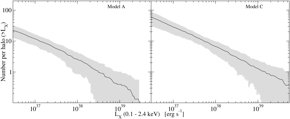
Figure 10: Cumulative X-ray luminosity functions for a $1.6\times 10^{12}$${\rm M}_{\odot}~{}$halo. The shaded area is the standard deviation around the mean number given by the lines. Model A is consistent with the absence of MBH sources more luminous than $10^{38}{\rm erg~{}s}^{-1}$ in the Milky-Way halo, while for model C this represents a $\sim 1.5$-$\sigma$ deviation.

For all known dwarf satellites of the Milky Way, the X-ray luminosity from the cores does not exceed $\sim 10^{37}{\rm erg~{}s}^{-1}$, and typically it is much lower. However, for the larger satellites the situation is different. For the Large Magellanic Cloud (LMC), for example, Kahabka (2002) finds a number of sources at X-ray luminosities larger than $10^{38}{\rm erg~{}s}^{-1}$ that have been classified as binary systems. Since the classification of binaries has been done on the basis of X-ray hardness ratios this leaves open the possibility that some of them could be accreting MBHs.

5 Summary and Conclusions

We have examined the observational consequences of a population of free-floating MBHs in galactic haloes. Both our predictions and the observations of such sources are highly uncertain. In our models, neither the mass nor the abundance or spatial distribution of MBHs allows for a unique identification by a single type of observation alone. As far as optical and X-ray signatures are concerned, MBHs could be numerous enough to differentiate them from the expected count of background sources. On the other hand, even for optimistic choices of the model parameters, the mass and accretion rates predicted are not large enough for the accretion luminosity of MBHs to be of a significantly different from that of XRBs. Forthcoming data from Chandra and XMM should allow for better spectral modelling of individual sources, which may resolve this ambiguity.

We have shown that our predicted sources, particularly from model A, could account for a large fraction of the bright emitters inferred from observations. The observed X-ray luminosity is determined by fitting a spectral model to the detected count rate. Depending on the model fitted the resulting luminosity can differ by a factor of order unity, which we have deemed sufficiently accurate to compare with predictions. This uncertainty is probably less significant than that arising from the assumption made about the intervening absorbing column densities, which have a strong impact on the counts of soft X-ray photons.

However, while different spectral models may yield similar luminosities they make significantly different assumptions about the underlying emission process and ultimately the nature of the ULX source. Typical fitting models include a multi-colour disk (MCD) and/or a power law, which have the advantage of being specified by few parameters. In most cases the colour temperature of the MCD implies a $\sim 1-10$ ${\rm M}_{\odot}~{}$BH emitting at or above the Eddington rate. It seems that the ADAF model applied to sub-Eddington accreting MBHs can match not only the X-ray luminosities but also spectral range of detected counts of ULXs. We therefore propose to routinely include ADAF models in spectral fits to X-ray observations.

ADAF models do involve one or two more key parameters, which may introduce degeneracies when used to fit X-ray data alone. The advantage is that for a single (as opposed to binary) MBH, ADAFs also predict the spectrum in the optical regime and as well as the existence of a correlation of the radio and X-ray fluxes. Consequently, observations in these bands could help break the degeneracy arising from the increased number of parameters. In contrast for binaries these bands may carry the spectral contribution of the visible companion, accounting for which adds more parameters, too. To fit the overall spectrum ADAFs and composite disk models for binary systems thus seem equally well placed.

Because of the absorption problem optical follow-ups are likely to yield best results for ULXs that are observed at high galactic latitudes to avoid the effect of the Galactic disk. For such ULXs optical data could help distinguish between MBHs and binary systems for sources placed within galaxies. To test the prediction of MBHs in the dark matter haloes outside galaxies and distinguish them from background AGN requires a systematic survey of X-ray point sources and optical follow-ups in fields around galaxies.
Our results in particular are

• We have applied a thin disk and ADAF to model the spectral signature of accreting MBHs. Applying this, we predict a few ULXs on average per galaxy halo. This is not consistent with observations, and therefore indicates either that our predicted accretion rates are somewhat too high, or that thin disk emission is shut off.

• B and V band magnitudes reach -10, or -15 when a thin disk is included. Because of absorption these are probably more useful for follow-ups.

• For ADAF accretion alone we match the slope of the luminosity function for one statistical sample of observations, and both, slope and normalisation for another one. On average we expect to find one ULX in a Milky-Way sized galaxy, although, the actual absence of one in the Milky-Way is consistent with our predictions.

• We did not find any luminosity segregation in the MBH sources. In general, MBHs are distributed over a somewhat larger range of radii than observed ULXs, but this may be partly due to observational selection.

While many ULXs are clearly linked to star formation and young objects such as high-mass XRBs, it is not clear that all ULXs need correspond to the same physical sources. We have shown that MBHs provide an alternative explanation for ULXs, and could plausibly account for an appreciable fraction of observed systems, at least in terms of the slope and normalisation of typical X-ray luminosity functions. MBHs might be particularly interesting candidates to explain ULXs in ellipticals, or those seen at large distances from star-forming regions in spirals.

The accretion luminosities predicted here are depend sensitively on the mass of MBHs and on the density of material surrounding these systems. As explained in this paper and in paper I, we calculate these quantities by assuming that seeds merge together efficiently, and that they retain around them a core of roughly galactic density. If merging does not proceed efficiently and we ignore any significant mass increase through gas accretion, then most MBHs will have roughly the initial seed mass and X-ray luminosities will never reach the ULX range. Similarly, if the debris in the core around MBHs had a much lower density then they could easily escape detection.

The luminosities of accreting MBHs in individual bands also depend on the parameters of the particular spectral model used. For the ADAF model, however, the predicted X-ray luminosity is generally proportional to the bolometric luminosity. That means we can restate our results more generally by saying that if MBHs emit a reasonable fraction of their bolometric luminosity in X-rays, they can account for many of the observed ULXs. For the ADAF model the fraction of the luminosity emitted in X-rays is predicted to be fairly high, but in general we can keep this fraction as a free parameter encapsulating the overall uncertainty arising from the accretion rate and the particular spectral model used.

References

- [Abel, Bryan & Norman 2000] Abel T., Bryan G.L., Norman M.L., 2000, ApJ, 540, 39
- [Ball, Narayan & Quataert 2001] Ball G.H., Narayan R., Quataert E., 2001, ApJ, 552, 221
- [Beasley et al. 2002] Beasley M.A., Baugh C.M., Forbes D.A., Sharples R.M. et al. ,2002, MNRAS, 333, 383
- [Bondi & Hoyle 1944] Bondi H., Hoyle F., 1944, MNRAS, 104, 273
- [Bondi 1952] Bondi H., 1952, MNRAS, 112, 195
- [Bromm, Coppi & Larson 2002] Bromm V., Coppi P.S., Larson R.B., 2002, ApJ, 564, 23
- [Chisholm, Dodelson & Kolb 2003] Chisholm J.R., Dodelson S., Kolb E.W., 2003, ApJ, 596, 437
- [Colbert & Mushotzky 1999] Colbert E.J.M., Mushotzky R.F., 1999, ApJ, 519, 89
- [Colbert & Ptak 2002] Colbert E.J.M., Ptak A.F., 2002, ApJ, 143, S25
- [Ebisuzaki et al. 2001] Ebisuzaki T. et al. , 2001, ApJ, 562, L19
- [Fabbiano 1989] Fabbiano G., 1989, Ann. Rev. A & A, 27, 87
- [Frank, King, & Raine 1985] Frank, J., King, A. R., & Raine, D. J., 1985, Accretion Power in Astrophysics, Cambridge Univ. Press, Cambridge, p. 84
- [Fuller & Couchman 2000] Fuller T.M., Couchman H.M.P., 2000, ApJ, 544, 6
- [Grimm, Gilfanov & Sunyaev 2002] Grimm L.-H., Gilfanov M., Sunyaev R., 2002, A&A, 391, 923
- [Heger et al. 2002] Heger A., Woosley S., Baraffe I., Abel T. 2002, in Proc. MPA/ESO, Lighthouses of the Universe: The Most Luminous Celestial Objects and Their Use for Cosmology. ESO, Garching, p. 369
- [Holt et al. 2003] Holt S.S., Schlegel E.M., Hwang U., Petre R., 2003, ApJ, 588, 792
- [Hutchings et al. 2002] Hutchings R.M., Santoro F., Thomas P.A., Couchman H.M.P., 2002, MNRAS, 330, 927
- [Islam, Taylor & Silk 2003, paper I herafter] Islam R.R., Taylor J.E., Silk J., MNRAS submitted, astro-ph/0307171
- [Ichimaru 1977] Ichimaru S., 1977, ApJ, 214, 840
- [Ipser & Price 1977] Ipser J.R., Price R.H., 1977, ApJ, 216, 578
- [Jeltema & Canizares 2003] Jeltema T.E., Canizares C.R., 2003, ApJ, 585, 756
- [Kaaret 2002] Kaaret P., 2002, ApJ, 578, 114
- [Kahabka 2002] Kahabka P., 2002, A&A, 388, 100
- [Kilgard et al. 2002] Kilgard, R. E., Kaaret, P., Krauss, M. I., Prestwich, A. H., Raley, M. T., Zezas, A., 2002, ApJ, 573, 138
- [King et al. 2001] King, A. R., Davies, M. B., Ward, M. J., Fabbiano, G., Elvis, M., et al. 2001, ApJ, 552, L109
- [Kormendy & Gebhardt 2001] Kormendy J & Gebhardt K., 2001, in Wheeler J.C., Martel H., eds, Proc. AIP Symp. 586, XX Texas Syposium on Relativistic Astrophysics, AIP, New York, p. 363
- [Larson 1981] Larson R.B, 1981, MNRAS, 194, 809
- [Lin & Murray 2002] Lin D.N.C., Murray S.D., 2002, in Nomoto K., Truran J. W., eds, Proc. IAU Symp. Vol. 187, Cosmic Chemical Evolution. Kluwer Academic, Dordrecht, p. 165
- [Mahadevan 1997] Mahadevan R., 1997, ApJ, 477, 585
- [Makishima et al. 2000] Makishima K., Kubota A., Mizuno T., Ohnishi T., 2000, ApJ, 535, 632
- [Manmoto, Mineshige & Kusunose 1997] Manmoto T., Mineshige S, Kusunose M., 1997, ApJ, 489, 791
- [Markowitz et al. 2003] Markowitz A., et al. , 2003, ApJ, 593, 96
- [Miller & Hamilton 2002] Miller M.C., Hamilton D.P., 2002, MNRAS, 330, 232
- [Mouri & Taniguchi 2002] Mouri H., Taniguchi Y., 2002, ApJ, 566, L17
- [Narayan & Yi 1994] Narayan R., Yi I., 1994, ApJ, 428, L13
- [Narayan, Mhadevan, Quetaert 1998] Narayan R., Mahadevan R., Quataert E., 1998, in Abramowicz M.A., Bjornsson G.,Pringle J.E., eds, The Theory of Black Hole Accretion Disks. Cambridge Univ. Press, Cambridge, p. 148
- [Omukai & Palla 2001] Omukai K., Palla F., 2001, ApJ, 561, L55
- [Portegies Zwart & McMillan 2002] Portegies Zwart S.F., McMillan S.L.W., 2002, ApJ, 576, 899
- [Rees et al. 1982] Rees M.J., Begelman M.C., Blandford R.D., Phinney E.S., 1982, Nature, 295, 17
- [Roberts & Warwick 2000] Roberts T.P., Warwick R.S., 2000, MNRAS, 315, 98
- [Schlegel, Finkbeiner & Davis 1998] Schlegel D.J., Finkbeiner D.P., Davis M. 1998, ApJ, 500, 525
- [Shakura & Sunyaev 1973] Shakura N., Sunyaev R.A., 1973, A&A, 24, 377
- [Smith & Wilson 2003] Smith D.A., Wilson A.S., 2003, ApJ, 591, 138
- [Swartz et al. 2003] Swartz D.A., Ghosh K.K., McCollough M.L., Pannuti T.G., 2003, ApJ, 144, 213
- [Swartz, Ghosh & Tennant 2003] Swartz D.A., Ghosh K.K., Tennant A.F., AAS meeting 201, 54.13 (2003)
- [Tegmark et al. 1997] Tegmark, M., Silk, J., Rees, M. J., Blanchard, A., Abel, T., & Palla, F., 1997, ApJ, 474, 1
- [Tennant et al. 2001] Tennant, A. F., Wu, K., Ghosh, K. K., Kolodziejczak, J. J., & Swartz, D. A., 2001, ApJ, 549, L43
- [Wang 2002] Wang Q.D., 2002, MNRAS, 332, 764
- [Zang & Meurs 2001] Zang Z., Meurs E.J.A., 2001, ApJ, 556, 24
- [Zezas & Fabbiano 2002] Zezas A., Fabbiano G., 2002, ApJ, 577, 726