Massive black hole remnants of the first stars III: observational signatures from the past

Abstract

The first stars forming in minihaloes at redshifts greater than 20 may have been very massive and could have left behind massive black hole (MBH) remnants. In previous papers we investigated the hierarchical merging of these ‘seed’ MBHs and their associated haloes, using a semi-analytical approach consisting of a hierarchical merger tree algorithm and explicit prescriptions for the dynamics of merged substructure inside a larger host halo following a merger. We also estimated accretion luminosities for these MBHs and found them to be consistent with observations of ultra-luminous X-ray point sources. Here we compute the strength of gravitational wave events as MBHs merge to form the more massive black holes that we predict reside in galaxy haloes today. If MBHs merge efficiently, we predict that as many as $10^{4}$–$10^{5}$ events per year may fall within the sensitivity limits of the proposed LISA gravitational wave observatory. The collapse of the first massive stars to form MBHs may also be accompanied by gamma-ray bursts (GRBs). If this is the case and if GRBs are observable out to the redshifts of first star formation, we predict that about $10^{5}$–$10^{6}$ GRBs per year could be detected. As merging MBH binaries reach their last stable orbits before final coalescence a fraction of the gravitational wave energy may be released as a pulse of gamma rays (for instance, through interaction with material enveloping a merging MBH binary). This fraction has to be larger than about $10^{-2}$ for MBH mergers to account for some beamed GRBs, and greater than $10^{-6}$ for the gamma rays to be detectable out to cosmological distances with upcoming GRB detector missions.

1 Introduction

There is increasing speculation that the first generation of stars in the universe may have been extremely massive, and that some of these objects could have collapsed directly to massive black holes (MBHs) at the end of a brief stellar lifetime. If these objects do form in the early universe, then they may provide a unique opportunity to study primordial star formation, through their gravitational wave or gamma-ray emission.

Recent semi-analytic [Hutchings  et al. 2002, Fuller & Couchman 2000, Tegmark  et al. 1997] and numerical studies [Bromm, Coppi & Larson 2002, Abel, Bryan & Norman 2000] suggest that the first stars in the universe formed inside dense baryonic cores, as they cooled and collapsed within dark matter haloes at very high redshift. For a standard $\Lambda$CDM cosmology, these minihaloes are estimated to have had masses in the range $M_{min}\sim 10^{5}$–$10^{6}~{}h^{-1}$ ${\rm M}_{\odot}$, and to have collapsed at redshifts $z_{\rm collapse}\sim 20$–$30$ or higher. Since these first star-forming clouds contained essentially no metals, gas cooling would proceed much more slowly in these systems than in present-day molecular clouds. As a result, they may have collapsed smoothly and without fragmentation, producing dense cores much more massive than the proto-stellar cores observed in star-formation regions today. Assuming nuclei within these cores accreted the surrounding material efficiently, the result would be a first generation of protostars with masses as great as $10^{3}$ ${\rm M}_{\odot}$ [Bromm, Coppi & Larson 2002, Omukai & Palla 2001].

As yet, nothing definite is known about the subsequent evolution of such objects. However, their large masses would probably result in many of them ending up as MBHs with little intervening mass loss – for systems in this mass range, gravity is so strong that there is no ejection of material from the system in a final supernova bounce [Heger et al. 2002]. This high-redshift population of MBHs is interesting as a source of seeds for the formation of the supermassive black holes (SMBHs) seen at the centres of galaxies at the present-day. Furthermore, the initial collapse of these objects or mergers between them might be detectable through the resulting gamma-ray or gravitational wave emission. This would provide a direct test of the physics of primordial star formation and the high-redshift universe.

In a previous paper [Islam, Taylor & Silk 2003, herafter paper I] we used a semi-analytical model of galaxy formation to follow the evolution of MBHs as they merge together hierarchically, along with their associated haloes. The code we used combines a Monte-Carlo algorithm to generate halo merger trees with analytical descriptions for the main dynamical processes – dynamical friction, tidal stripping, and tidal heating – that determine the evolution of merged remnants within a galaxy halo. We introduce seeds into the code by assuming that in each minihalo forming before a redshift $z_{\rm collapse}$, a single MBH forms as the end result of primordial star formation.

For our computations, we considered four different sets of values for the parameters $\nu_{pk}$ and $M_{\bullet,seed}$, which fix the abundance and the mass of the seeds respectively. These values are summarised in table 1. Our choice of a seed MBH mass of 260 ${\rm M}_{\odot}$ is motivated by the result of Heger (2002) that massive stars above this mass will not experience a supernova at the end of their lives, but instead will collapse directly to a MBH of essentially the same mass.

Table 1: The mass of seed MBHs, and the height of the peaks in the initial density field in which they formed, for the four models considered. The collapse redshift $z_{\rm collapse}$ is the epoch when peaks of height $\nu_{pk}$ first cross the cooling threshold (see paper I).

Model	$M_{\bullet,seed}$	peak height $\nu_{pk}$	$z_{\rm collapse}$
A	260 ${\rm M}_{\odot}$	3.0	24.6
B	1300 ${\rm M}_{\odot}$	3.0	24.6
C	260 ${\rm M}_{\odot}$	2.5	19.8
D	260 ${\rm M}_{\odot}$	3.5	29.4

In paper I we investigated the abundance of MBHs in present-day galaxies as a result of this process of hierarchical merging and dynamical evolution. For these MBHs we estimated the X-ray accretion luminosities using two different accretion models and found that they could well account for many of the ultra-luminous off-centre X-ray point sources that are observed in local galaxies[Islam, Taylor & Silk 2003, herafter paper II].

In this paper we investigate how our model could be tested at high redshifts. In particular, we predict the number of gravitational wave events arising from MBH mergers that should be detectable with the upcoming LISA mission. Conversely, observations of gravitational wave events could then be used to constrain the merging history of MBHs and provide limits on the abundance of these objects at cosmological distances and to very high redshifts (see also Haehnelt (1994) , Menou, Haiman & Narayanan (2001) ). If the collapse of the first massive stars to form MBHs is accompanied by gamma-ray bursts (GRBs), then observations of GRBs may allow us to directly probe the epoch of first star formation at redshifts larger than 20. Here we estimate the number of GRB events that could be observed per year if GRBs are detectable out to the redshifts of first star formation.

The structure of the paper is as follows. In section 2 we compute the number of MBH mergers and the number of associated gravitational wave events. Section 3 considers the expected number of GRBs from collapsing massive population III stars, as well as the possibility of gamma-ray emission in the wake of MBH mergers. We discuss and summarise our findings in section 4

2 Gravitational waves from SMBH-MBH mergers

There are essentially two types of gravitational waves that are emitted at different stages in the evolution of the scenario we are considering. The first of these are ‘burst’ signals associated with the collapse of massive population III stars into MBHs. In our model, these are events occurring at very high redshifts $>$ 20 for a cosmological abundance of massive population III stars, so we expect a stochastic gravitational wave background to be generated [Schneider  et al. 2000, de Araujo, Miranda & Aguiar 2002]. Although statistical limits can be imposed, the particular number and strength of burst signals created in this way does depend on the initial number and masses of collapsing stars and the collapse mechanism.

In contrast periodic signals, albeit with changing frequency, are emitted during the subsequent merger of MBHs to form more massive BHs. Compared to the burst signals from collapsing population III stars, the mergers of MBHs produce stronger waves due the higher total mass of the gravitationally interacting system. As a result gravity waves could be detected for individual merger events. The signals from merger events can be further subdivided into signals associated with the inspiral phase, actual coalescence and subsequent ringdown [Flanagan & Hughes 1998]. Of these, the inspiral phase is the longest and thus most likely to detect. In the following we will be exclusively concerned with the gravitational waves emitted during this phase. These are also referred to as ‘chirp’ signals, due to the fact that during inspiral the distance between the BHs in the merging binary decreases continuously as energy is lost through gravity waves, resulting in the frequency of emitted waves rapidly sweeping upwards.

2.1 Gravitational Wave Amplitude

For any measurement of gravitational waves the most important pieces of information are the frequency and some measure of their amplitude, both of which will be functions of time. Because of the spin-2 nature of gravity, the first non-zero and largest term of the tensor describing the gravity wave induced perturbation of space-time is the quadrupole moment. This can be described by an overall dimensionless strain amplitude $h_{s}$. For periodic signals such as those emitted by a binary black hole system, this is given by [Thorne 1989]

$$h_{s}=8\left(\frac{2}{15}\right)^{1/2}\frac{G^{5/3}\mu_{12}}{c^{4}D(z)}(\pi M_{12}f_{gw})^{2/3}$$ (1)

where $f_{gw}$ is the frequency of gravitational waves, which in this case is just twice the orbital frequency of the binary; $M_{12}=M_{1}+M_{2}$ and $\mu_{12}=M_{1}M_{2}/M$, G is Newton’s constant and c the speed of light. $D(z)$, the distance to the binary, can be obtained by integrating the differential distance redshift relation

$$D(z)=\frac{c}{H_{0}}\int_{0}^{z}\frac{{\rm d}z^{\prime}}{(\Omega_{m}(1+z^{\prime})^{3}+\Omega_{\Lambda})^{-1/2}}$$ (2)

The effective strain amplitude measured at some characteristic frequency $f_{c}$ is further enhanced proportionally to the square root of the number of periods, n, that the binary emits at or near that frequency. For an inspiralling binary system whose frequency sweeps up, or ‘chirps’,in frequency (cf. below), $n\propto\mu_{12}^{-1/2}M_{12}^{-1/3}f_{c}^{-5/6}$ and the characteristic strain amplitude, $h_{c}$ is thus [Thorne 1989, Nakamura et al. 1997]

$$h_{c}=2.94\times 10^{-19}\left(\frac{M_{chirp}}{10^{3}{\rm M}_{\odot}}\right)^{5/6}\left(\frac{f_{c}}{{\rm Hz}}\right)^{-1/6}\left(\frac{D(z)}{10{\rm Mpc}}\right)^{-1}$$ (3)

where $f_{c}$ is the frequency of the wave signal, $r$ the distance from the merging binary and the ‘chirp’ mass $M_{chirp}$ accounts for the masses $M_{1}$ and $M_{2}$ of the binary constituents

$$M_{chirp}=\frac{(M_{1}M_{2})^{3/5}}{(M_{1}+M_{2})^{1/5}}=\mu_{12}^{3/5}M_{12}^{2/5}$$ (4)

Particularly at late times, most mergers in our model are between a massive central MBH and much lighter seed MBHs, so we can consider the problem in the limit that one of the merging binary constituents is much larger than the other. If we assign $M_{1}$ and $M_{2}$ to the masses of the central and inspiralling MBH respectively, $M_{1}\gg M_{2}$ and

$$M_{chirp}\approx M_{1}x^{3/5}$$ (5)

where $x=M_{2}/M_{1}$ denotes the mass ratio between the two masses.

The largest frequency at which a gravitational wave source can emit is determined by its light radius which in turn is dependent on its mass, and so in this case $f_{max}\approx 10{\rm~{}Hz}(10^{3}{\rm M}_{\odot}/M_{1})$. A lower limit on the characteristic wave amplitude is then

$$h_{c}\approx 2\times 10^{-19}\sqrt{x}\left(\frac{M_{1}}{10^{3}{\rm M}_{\odot}}\right)\left(\frac{D(z)}{10{\rm Mpc}}\right)^{-1}$$ (6)

2.2 Frequency of gravitational Waves

The proposed LISA (Laser Interferometer Space Antenna) gravitational wave observatory will be the only instrument capable of detecting gravity waves in the typical frequency range generated in the inspiral phase of a merging binary of massive black holes. A rough estimate of the maximum frequency of waves emitted by the merging binary is

$$f_{max}\sim 10{\rm~{}Hz}\frac{10^{3}{\rm M}_{\odot}}{M_{1}}$$ (7)

where $M_{1}$ is the more massive of the binary constituents.

For a binary on circular orbit, the frequency of the chirp signal can be described analytically. If the orbital radius is $a_{0}$ at time $t_{0}=0$, then the time for the binary constituents to spiral into each other is [Misner, Thorne & Wheeler 1973]

$$\tau_{0}=0.665\left(\frac{M_{12}}{10^{3}{\rm M}_{\odot}}\right)^{-2}\left(\frac{\mu_{12}}{10^{3}{\rm M}_{\odot}}\right)^{-1}\left(\frac{a_{0}}{10^{8}{\rm m}}\right)^{4}{\rm yr}$$ (8)

The frequency of the waves emitted at a later time $t$ is

$$f_{gw}=3.11\times 10^{-3}\left(\frac{M_{chirp}}{10^{3}{\rm M}_{\odot}}\right)^{-5/8}\left(\frac{\tau_{0}-t}{{\rm yr}}\right)^{-3/8}{\rm Hz}$$ (9)

Including the redshift $z$, the waves are then detected by LISA with a frequency

$$f_{gw}=\frac{3.11\times 10^{-3}}{(1+z)}\left(\frac{M_{chirp}}{10^{3}{\rm M}_{\odot}}\right)^{-5/8}\left(\frac{\tau_{0}-\frac{t}{1+z}}{{\rm yr}}\right)^{-3/8}{\rm Hz}$$ (10)

For the case that $M_{1}\gg M_{2}$, $\tau_{0}$ and $f_{gw}$ are approximately given by

$$\tau_{0}\approx\frac{0.665}{x}\left(\frac{M_{1}}{10^{3}{\rm M}_{\odot}}\right)^{-3}\left(\frac{a_{0}}{10^{8}{\rm m}}\right)^{4}{\rm yr}$$ (11)

$$f_{gw}\approx\frac{3.11\times 10^{-3}}{(1+z)}\left(\frac{M_{1}}{10^{3}{\rm M}_{\odot}}\right)^{-5/8}\left(x\frac{\tau_{0}-\frac{t}{1+z}}{{\rm yr}}\right)^{-3/8}{\rm Hz}$$ (12)

2.3 MBH Merger Efficiency

We have outlined above the main characteristics of the gravitational wave signals received from individual merger events. The formulae given estimate the amplitude and frequency averaged over all inclinations of the merger orbital plane.

For a merger event to actually occur the MBHs have to come within a distance where gravitational waves can efficiently reduce the orbital energy and allow the MBHs to spiral together and coalesce. However, this only happens at MBH separations that are very much smaller than the ones we are considering here (of order 10 - 100 pc).

For a MBH binary on a circular orbit to coalesce through gravitational wave emission within a Hubble time, the MBH separation, $a$, needs to satisfy [Peters 1964]

$$a~{}\leq~{}a_{gw} = \left(\frac{256~{}t_{hubble}~{}G^{3}~{}\mu_{12}~{}M_{1}^{2}}{5~{}c^{5}}\right)^{1/4}$$

$$\approx 4.5\times 10^{-6}\left(\frac{h}{0.7}\right)^{-1/4}\left(\frac{M_{1}}{260~{}M_{\odot}}\right)^{3/4}$$

$$\times\left(\frac{M_{2}(M_{1}+M_{2})^{2}}{M_{1}^{2}}\right)^{1/4}~{}{\rm pc}$$

At distances larger than this the common environment of the MBHs determines whether and how quickly the MBHs will be driven towards each other. If two MBHs come within a distance

$$a \mathrel{\hbox{\hbox to0.0pt{\hbox{\lower 4.0pt\hbox{$\sim$}}\hss}\hbox{$<$}}} a_{h}=\frac{G~{}M_{2}}{4~{}\sigma_{c}^{2}}$$

$$\approx 7.3\times 10^{-2}\left(\frac{M_{2}}{260M_{\odot}}\right)\left(\frac{\sigma_{c}}{200~{}{\rm km~{}s^{-1}}}\right)^{-2}~{}{\rm pc}$$

they form a ‘hard’ binary. Interactions with stars in the binary’s vicinity carry away energy from the binary with the result that the binary separation shrinks – the binary is said to ‘harden’. The time scale on which this happens is given by

$$t_{h}=\frac{\sigma_{c}}{G~{}\rho_{\star}~{}a~{}H_{h}}$$ (15)

where $H_{h}$ is the dimensionless hardening rate and is of the order $H_{h}\approx 15$ [Quinlan 1996]. In a fixed isothermal stellar background with a number density of stars, $\rho_{\star}=\sigma_{c}^{2}/(2~{}\pi Gr^{2})$ the hardening timescale starting at $a=a_{h}$ becomes

$$t_{h} = \frac{\pi~{}G~{}M_{2}}{2~{}\sigma_{c}^{3}~{}H_{h}}$$

$$\approx 1.44\times 10^{7}\left(\frac{M_{2}}{260~{}M_{\odot}}\right)\left(\frac{\sigma_{c}}{200~{}{\rm m~{}s^{-1}}}\right)^{-3}\left(\frac{H_{h}}{15}\right)^{-1}~{}{\rm yr}$$

As it stands this implies that the hardening timescale is proportional to the lighter MBH in the binary system. This makes sense: as the mass of $M_{2}$ increases the fraction of energy lost to any interacting star decreases. A light MBH binary therefore needs less stellar interactions to harden. However, this is only strictly valid if the stellar background is fixed. That is, we have ignored any depletion of the stellar density in the binary environment due to the interactions and resulting ejections of stars from the binary (see for example Milosavljevi c & Merritt (2001) ).

The hard binary stage can represent a bottleneck on the way to MBH mergers – particularly for very massive (S)MBHs, as dynamical friction is no longer significant but gravitational radiation not yet effective enough in further reducing the separation between the MBHs. However, both, the dynamical interaction with stars in the MBH binary’s vicinity as well as gas infall are likely to have the potential to quickly reduce the distance between the MBHs [Barnes & Hernquist 1996, Naab & Burkert 2001, Barnes 2002, Armitage & Natarajan 2002, Escala  et al.]. We do not quantify this effect, but note that the role of gas infall in this context is probably more important at early times when MBHs encounter each other more often in the wake of major mergers of two host haloes .

2.3.1 Dynamical friction at the centre of haloes

At still larger distances, dynamical friction is the main mechanism by which MBHs are drawn to the centre. The dynamical friction force is given by the Chandrasekhar formula [Binney & Tremaine 1987]

$$\frac{{\rm~{}d}{\bf v}_{sat}}{{\rm~{}d}t}=-16\pi^{2}{\rm ln}\Lambda_{c}G^{2}m(M_{sat}+m)\frac{\int_{0}^{v_{sat}}f(v^{\prime})v^{\prime 2}{\rm~{}d}v}{v^{3}_{sat}}{\bf v}_{sat}$$ (17)

where ${\bf v}_{sat}$ is the satellite velocity with respect to the host centre, $M_{sat}$ the satellite mass, $m$ is the mass of individual host halo particles, that have a distribution function $f(v)$, and ln $\Lambda_{c}={\rm ln}(b_{max}/b_{min})$ is the Coulomb logarithm, that is the ratio of maximum and minimum impact parameters, $b_{max}$ and $b_{min}$, of the host particles with respect to the satellite system.

This effect has been modelled in the numerical scheme using the semi-analytical dynamical friction timescale given by Colpi, Mayer & Governato (1999; see also Taylor & Babul 2004)

$$\tau_{df}=k\frac{(M_{host}/M_{sat})}{{~{}\rm ln}(M_{host}/M_{sat})}\epsilon^{0.4}\frac{P_{vir}}{2~{}\pi}$$ (18)

where $M_{host}$ and $M_{sat}$ denote the mass of the host and satellite haloes respectively and $P_{vir}$ is the circular orbital period at the virial radius of the host, and $k$ is a numerical constant. Colpi et al. (1999) find $k=1.2e\simeq 3.26$ for massive satellites in an isothermal potential with a constant-density core. We will use the value k = 2.4, found to match the infall times for massive satellites in a cuspy potential in the model of Taylor and Babul (2004). The circularity parameter $\epsilon=J(E)/J_{circ}(E)$ is the ratio of the angular momentum of the actual satellite orbit and that of a circular orbit with the same energy.

In the following we assume that this timescale dominates both the timescale for gravitational wave induced coalescence and that for overcoming the hard binary stage, which in principle can be very short due to the effects of gas and stellar dynamical processes.

In order to compute the time when a MBH merges with the central (S)MBH in the host we first establish the time when a satellite/MBH system sinks to an orbit with a radius less than the radius of the infall region. This is 1 per cent of the host virial radius at the time. At this point the satellite/MBH system in question has so far been considered as having ‘fallen to the centre’; following their dynamics to smaller radii was too expensive computationally.

To track infall more accurately, we add to this time a dynamical friction infall time, using eq.(18) and replacing the total host mass interior to the virial radius and the orbital period at the virial radius with the respective quantities at the outer radius of the infall region. This is also shown in figure 1 for a range of satellite to

Figure 1: Ratio of dynamical friction time to orbital period plotted against ratio of host mass interior to satellite orbit to satellite mass. From top to bottom the curves are for values of the circularity parameter $\epsilon=1.0,0.8,0.6,0.4,0.2$.

host mass ratios. The circular parameter $\epsilon$ is computed from the last orbit of the satellite system before it crossed into the infall region. The result is a more accurate estimate of the time when the actual merger occurs. As a result of the correction to the infall time we also inevitably change the order in which the MBHs merge with the centre. This in turn leads to a change in the growth history of the central (S)MBH and also to a slightly lower final mass of the SMBH, since there is now a small fraction of satellite MBH systems that do not merge with the centre within a Hubble time.

Figure 2: The figure shows the total mass of the host halo versus the mass of the central (S)MBH. For the (S)MBH mass we have taken account of the slightly altered growth history due to the addition of a dynamical friction infall time after satellite MBH systems have crossed the infall radius.

Figure 2 shows the host halo mass versus the resulting mass of the central (S)MBH for final halo masses of $1.6\times 10^{10,11,12}$ ${\rm M}_{\odot}$ and their lighter precursor haloes at higher redshifts. The data points from precursors of different final halo masses are recognisable by their accumulation near those final halo masses. Nevertheless, all data points lie on a line with a slope that is also consistent with the one we determined for the $M_{SMBH}-M_{bulge}$ relation in paper I. This indicates that the ratio of SMBH to halo mass does not depend significantly on the redshift.

We also made an important assumption regarding the actual mass of the satellite systems in which the MBHs are embedded. The semi-analytical code we used to follow the satellite dynamics considers every satellite naked if its mass has dropped to something less than about 0.3 per cent of its original mass . For all ‘naked’ MBH satellite systems arriving at the infall radius we have therefore assumed a mass equal to this limit. We do impose a lower limit of $3\times 10^{3}$${\rm M}_{\odot}$ for the mass of any naked satellite system, roughly corresponding to 1 per cent of the mass of the minihaloes and large enough for the presence of a baryonic core of the order the MBH mass. It is this remnant material of the satellite associated with an MBH that allows MBHs to the delivered to the centre efficiently by dynamical friction. This point has also been mentioned by Yu (2002) .

For the halo of final mass $1.6\times 10^{12}$ ${\rm M}_{\odot}$ we find the following. Of the satellite MBH systems crossing the infall radius about 96 per cent do arrive at the centre within a Hubble time. These MBHs contain 99 per cent of the mass of all MBHs in the infall region. If we reduce the satellite mass to 0.03 per cent of its original value and the lower limit to $3\times 10^{3}$${\rm M}_{\odot}$ we still find that 88 per cent of the MBHs in the infall region (accounting for 97 per cent of the mass) end up at the centre within a Hubble time. In haloes of lower final mass virtually all MBHs systems crossing the infall radius travel to the centre within a Hubble time.

2.3.2 Dynamical Friction and Gas Infall in Galaxy Mergers

MBHs with masses and orbits that would not allow them to travel to the centre within a Hubble time may still end up in the centre if the environment changes in a way that allows dynamical friction to act more efficiently. Mergers between galaxies of similar mass (‘major mergers’) through the accompanying violent dynamical processes may induce the dramatic changes to the matter distribution in the central region that we are looking for. Hydrodynamical simulations of mergers of gas rich galaxies [Barnes 2002, Barnes & Hernquist 1996, Naab & Burkert 2001] show that up to $60$ percent of the total gas mass of the two galaxies can end up within a region just a few hundred pc across at the centre of the merger remnant, thereby triggering starbursts and initiating the fuelling of quasars. This highly dense gaseous core should remain until feedback from star formation, supernovae or quasar activity begins to drive it out again.

We have already identified gas infall as a potential mechanism for accelerating the evolution of a hard MBH binary. We now look at how this effect can also boost the efficiency of dynamical friction as MBHs move in the central region of the merger remnant. If the respective central-kpc region of each galaxy ends up within a kpc or so of the new centre of the remnant after merging, then so will any MBHs that were present within a kpc of the original galactic centres. This seems reasonable since the central regions, sitting deepest in the gravitational potential of each galaxy, will be most stable to tidal disruption. It is plausible that MBHs originally present there travel along the line connecting the centres of the merging galaxies, towards the new global potential minimum of the merger remnant.

This migration of MBHs could be accelerated by the rapid infall of large amounts of gas into a small core region. The question then is whether the density and the bulk inflow velocity of the gas is sufficient to accelerate any orbiting MBH towards the centre via dynamical friction. The complex dynamical events and rapidly varying geometry make it difficult to determine accurately any radial bulk inflow velocities and gas densities as they evolve with time, and particularly so in the core central region, where things are made more difficult by the resolution limits of the simulations. Even a rough estimate of these quantities may already yield useful constraints for our problem, however. In the following we try to estimate the timescale for infalling gas to carry two MBHs towards the centre by dynamical friction before the gas leaves the central region again.

For two disk galaxies, each having a total mass $M_{gal}=2.75\times 10^{11}$ ${\rm M}_{\odot}$ and gas mass $M_{gas}=5.5\times 10^{9}$ ${\rm M}_{\odot}$ in the disk and initial pericentric separation of $R_{p}=8{\rm kpc}$, Barnes & Hernquist (1996) find that roughly $60$ percent of the total gas mass end up within a region approximately $100$ pc in radius some 1.5 Gyrs later. Assuming the centre of the merger remnant will be half-way between the galaxies at initial separation and the gas flows towards this point along the line connecting the merging galaxy centres, the average inflow velocity of the gas is $v_{flow}\sim 4{\rm kpc}/1.5{\rm Gyr}\approx 2.7~{}{\rm kms}^{-1}$. Further we assume that the gas density in the flow is of the same order as the final gas density in the centre, i.e. $\rho_{flow}\sim 7\times 10^{9}M_{\odot}/(4\times 100^{3}{\rm pc^{3}})\approx 1.6\times 10^{3}{\rm Mpc~{}pc^{-3}}$. Putting this into eq. 17 we find that the MBHs get accelerated to within 1 per cent of $v_{flow}$ in a time

$$\tau_{df,flow}\sim 2\times 10^{6}\left(\frac{M_{\bullet}}{260~{}M_{\odot}}\right)^{-1}~{}{\rm yr}$$ (19)

Even for seed mass MBHs, this time is negligible compared to the time scale of the inflow of about 1–2 Gyrs. Although we do not know what exactly will happen to the MBHs once they have entered the central 100 pc of the remnant, gas inflow seems at least capable of efficiently transporting MBHs from the outer radius of the infall region ($\sim 1{\rm kpc}$, for galaxies of this size) down to at least 100 pc. This holds in particular for MBHs that previously would not have been able to spiral anywhere near the centre.

2.3.3 Multiple MBH interactions

Up to now we have implicitly assumed that a MBH binary merges before it forms a new binary with another incoming MBH. However, given the number of inspiralling MBHs involved it is possible that there are cases where incoming MBHs will find another MBH binary that has not yet merged. If the binary system and the incoming third MBH come close enough then there is a possibility that one of the MBHs will be ejected [Begelman, Blandford & Rees 1980]. The required proximity of an incoming MBH and MBH binary is facilitated primarily by major mergers. This will be the case particularly at high redshifts, as most MBH interactions will be between MBHs with similar masses (of the order of the MBH seed mass), which also implies similar masses of their associated haloes.

As far as our model is concerned we have not incorporated the possibility of triple interactions in our results. We assume that stellar and gas dynamical effects in the wake of major mergers always lead to swift merging of MBH binaries, primarily through accelerating evolution of the hard binary stage. Here we consider what happens if we drop this assumption. For the case that stellar and gas dynamics have no mitigating effect, we can determine a rough limit for the number of triple interactions and resulting sling-shot ejections of MBHs.

Figure 3: Rates of halo MBHs merging with central (S)MBH, as a function of redshift. Results are shown for models A and C and for final halo masses of $1.6\times 10^{12,11,10}$${\rm M}_{\odot}$ (three sets of curves, from top to bottom). The dashed curves represent the same best fits to the data scaled by a factor corresponding to the different final halo mass (see text).

In figure 3 we show the number of mergers per unit time ($10^{6}$ yr) for model A and C. From top to bottom the curves are for $1.6\times 10^{12,11,10}$${\rm M}_{\odot}$ haloes. The dashed lines are the best fits. Let us consider the largest merger rate, which we find at $z\sim 5-10$ in the precursors of haloes with final mass $1.6\times 10^{12}$${\rm M}_{\odot}$. The rate is ${\rm~{}d}N_{merge}/{\rm~{}d}t\sim 0.07{\rm~{}Myr}^{-1}$ implying that two MBHs arrive at the centre within $\sim 15$ Myrs. For the lowest rates ${\rm~{}d}N_{merge}/{\rm~{}d}t\sim 0.001{\rm~{}Myr}^{-1}$ two MBHs would reach the centre within about a Gyr. These timescales would have to be compared with the hardening time of a MBH binary at the centre to determine the likelihood of a triple interaction. Yu (2002) finds that the hardening timescale can be significantly larger for equal mass binary systems, which again is more likely to be the case at very high redshifts.

Although the central halo MBH merger rate as shown in figure 3 is highly uncertain at high redshifts, there is a clear declining trend towards high redshifts. Consequently we would expect multiple MBH interactions to be less important. Overall, this is different from Volonteri  et al. (2003) , who find that there is a very significant probability for triple interactions. One important reason for this discrepancy is that they explicitly did not take into account tidal stripping of satellite systems and the resulting increase in the dynamical friction infall timescale. When MBHs are involved in triple interactions, they find that those MBHs that get ejected MBH will actually leave the galaxy (remnant) altogether [Volonteri, Haardt & Madau 2003]. These ejected MBHs could thus constitute a population of inter-galactic MBHs. Due to the nature of the process these MBHs will be mostly seed mass MBHs and will have been stripped naked, so that they will be virtually impossible to detect in the IGM.

The overall result is then, that while the formation of multiple MBH systems is possible, the probability of such events is likely less important than analytical arguments suggest. Previous estimates typically did not account for the tidal stripping of infalling satellites let alone their detailed dynamical evolution, but also the role of gas dynamics at the centre. The first effect implies that the rate at which MBHs arrive from the outer parts of the halo at the halo centre is lower, whereas the latter means that once MBHs have arrived at the centre, they form a binary that coalesces faster. In the light of this, we believe our assumption of efficient merging to be justified, particularly at redshifts $\mathrel{\hbox{\hbox to0.0pt{\hbox{\lower 4.0pt\hbox{$\sim$}}\hss}\hbox{$<$}}}15$ where MBHs mergers actually produce a strong enough gravitational wave signature that could be detected as we will see in the next section.

2.4 Rate of SMBH-MBH mergers

Figure 4: Rates of halo MBHs merging with central (S)MBH, as a function of redshift. Results are shown for models A and C and final halo mass of $1.6\times 10^{12}$${\rm M}_{\odot}$ with the dashed line representing a best fit. From top to bottom, the three sets of curves show the contribution of events with dimensionless strain amplitudes above a given value as shown.

We now attempt to obtain the cumulative signal of all mergers. To do this we essentially need to integrate over the mass function of haloes times the number of mergers per halo and finally integrate again over the relevant redshift ranges.

In what follows, we will only consider models A and C. In model D the rate of mergers is too low to derive a meaningful estimate of the average merger rate per halo, and consequently the total rate of events received from across the sky. Model B only differs from A in that it has a larger seed MBH mass. We do not expect this to make a significant difference when it comes to mergers with the centre. When calculating the dynamical friction time from the point the MBH systems cross the infall radius (cf. section 2.3.1), we assumed the MBH satellite system’s mass to be $\sim 0.3$ per cent of the original satellite mass. The difference in the satellite’s MBH mass in model A and C is thus insignificant. The larger MBH mass in model B will also only lead to very slightly increased strain amplitudes when MBHs eventually merge.

The number of MBH mergers per halo is shown in figure 3 for models A and C. The dashed lines represent a single cubic-polynomial fit in log space that is multiplied with a simple scaling factor for different halo masses.

$$\frac{{\rm~{}d}n_{merge}(M_{h,0},z)}{{\rm~{}d}t} = \left(\frac{M_{h,0}}{1.6\times 10^{12}M_{\odot}}\right)^{\beta}$$ (20)

$$\times e^{{\rm b}_{0}+{\rm b}_{1}~{}z+{\rm b}_{2}~{}z^{2}+{\rm b}_{3}~{}z^{3}}~{}{\rm Myr}^{-1}$$

where $M_{h,0}$ denotes final halo mass. For model A we find $({\rm b}_{0},{\rm b}_{1},{\rm b}_{2},{\rm b}_{3},\beta)=(-3.75,0.12,0.022,-2.63\times 10^{-3},\frac{5}{9})$, while for model C we find $(-3.52,0.145,7.5\times 10^{-3},-1.57\times 10^{-3},\frac{1}{2})$. In this form the merger rate can now simply be divided into a product of a redshift dependent part, $u(z)$, and another one scaling with final halo mass

$$\frac{{\rm~{}d}n_{merge}}{{\rm~{}d}t}(M_{h,0},z)=\left(\frac{M_{h,0}}{1.6\times 10^{12}M_{\odot}}\right)^{\beta}~{}u(z)$$ (21)

Figure 4 shows the merger rate per halo with strain amplitudes $h_{c}>10^{-21}$ and $3\times 10^{-21}$ for a final halo mass of $1.6\times 10^{12}$ ${\rm M}_{\odot}$ only. While the best fit parameters change accordingly, we have assumed that the scaling with halo mass, as parametrised by $\beta$, remains the same. Although we have not explicitly stated any error bars, uncertainties will be quite large, since the merger rate per halo is determined by averaging over individual merger events occurring over large timescales. The only way of reducing this uncertainty is to run a significantly larger number of merger trees.

When determining $h_{c}$, we assume that the merging MBHs emit waves at the maximum frequency which is only expected to occur very briefly towards the end of the inspiral phase due to the rapid sweeping up in frequency. This, however, should not affect our result significantly, since $h_{c}$ depends only weakly on the frequency (cf. equation (3)).

Using the merger rate per halo we can already determine as a function of epoch a lower limit to the rate, ${\rm d}\nu_{rec}$ of received SMBH-MBH merger events.

$$\frac{{\rm d}\nu_{rec}(z)}{{\rm d}V} > \frac{1}{1+z}$$

$$\times\int_{M_{h,min}}^{\infty}\frac{{\rm d}n_{h}}{{\rm d}M_{h,0}}\frac{{\rm~{}d}n_{merge}}{{\rm~{}d}t}(M_{h,0},z)~{}{\rm d}M_{h,0}$$

$$= \frac{u(z)}{1+z}$$

$$\times\int_{M_{h,min}}^{\infty}\frac{{\rm d}n_{h,0}}{{\rm d}M_{h,0}}\left(\frac{M_{h,0}}{1.6\times 10^{12}M_{\odot}}\right)^{\beta}~{}{\rm d}M_{h,0}$$

where $V$ denotes volume and (1 + z) accounts for the redshift induced reduction in the rate of received events. ${\rm d}n_{h}/{\rm d}M_{h,0}$ is the differential mass function of haloes of mass $M_{h,0}$

$$\frac{{\rm d}n_{h}}{{\rm d}M_{h,0}}=\sqrt{\frac{2}{\pi}}\frac{\rho_{0}}{M_{h,0}}\left|\frac{{\rm d}{\rm ln}\sigma}{{\rm d}{\rm~{}ln}M_{h,0}}\right|\frac{\delta_{c}}{\sigma(M_{h,0})}{\rm exp}\left[\frac{-\delta_{c}^{2}}{2\sigma(M_{h,0})^{2}}\right]$$

where $\rho_{0}$ is the present-day cosmic matter density, $\sigma(M_{h,0})$ is the variance in the linear matter density field on scales corresponding to mass $M_{h,0}$, and $\delta_{c}$ is the critical overdensity for collapse.

Equation 2.4 is a lower limit, as it only considers mergers in the main trunk of the tree that grows to become a single halo of mass $M_{h}$ at $z=0$. To account for the mergers in side branches before they become incorporated in the main trunk of the tree the Press-Schechter (PS) mass function, which we had only computed for final halo masses above, needs to be replaced by the redshift dependent mass function. In addition we need to re-express the redshift dependent MBH merger rate per halo in terms of the halo mass at the redshift concerned. From our simulations we found that the average mass of a halo at redshift $z$, given that it grows into a halo of final mass $M_{h,0}$ today, can be approximated by

$$M_{h}(z)=M_{h}(M_{h,0},z)\approx{~{}\rm exp}\left[12+\tilde{m}-0.04~{}\tilde{m}~{}z\right]$$ (23)

where $\tilde{m}=11.5+{~{}\rm ln}\left(\frac{M_{h,0}}{1.6\times 10^{10}M_{\odot}}\right)$. We can now substitute this into equation 21 to eliminate the dependence on $M_{h,0}$ and obtain

$$\frac{{\rm~{}d}n_{merge}}{{\rm~{}d}t}(M_{h},z)=\left[10^{-7}\times\left(\frac{M_{h}}{1.6\times 10^{5}M_{\odot}}\right)^{\frac{1}{1-0.04z}}\right]^{\beta}~{}u(z)$$ (24)

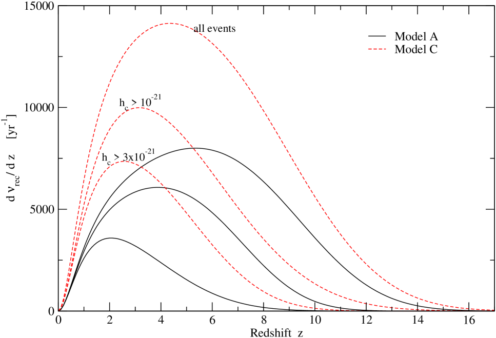
Figure 5: Redshift dependent rate of received merger events for models A and C. From top to bottom, the three sets show the contribution from all events and those with dimensionless strain amplitudes above $10^{-21}$ and $3\times 10^{-21}$ respectively.

The lower integration limit in eq 2.4 is determined by the minimum mass of haloes that harbour central MBHs. This mass has to be at least of order $10^{7}$ ${\rm M}_{\odot}$, since we argued above that only at this mass has every halo acquired one seed MBH. This is important since we have implicitly identified the number density of haloes with that of central MBHs.

If we now multiply $\frac{{\rm d}\nu_{rec}(z)}{{\rm d}V}$ with the volume of a spherical shell at radius $D(z)$ we obtain the total rate of events, d $\nu_{rec}(z)$, received from sources at distance $D(z)$ to $D(z)+{\rm d}D$

$${\rm d}\nu_{rec}(z)=\frac{{\rm d}\nu_{rec}(z)}{{\rm d}V}4\pi D(z)^{2}{\rm d}D$$ (25)

The resulting differential redshift distribution of the received rate of events is shown in figure 5, where we have also shown the contribution from events with associated dimensionless strain amplitudes $h_{c}$ above $10^{-21}$ and $3\times 10^{-21}$. The latter is based on the fits to the merger rate per halo shown in figure 4. Again, the errors are quite large and are difficult to quantify precisely, primarily because of the uncertainties in the merger rate per halo to which we now also have to add the uncertainty in the halo mass scaling, which we described by a power law with index $\beta$.

This differential distribution can then be integrated over all redshifts to obtain the total number of merger events received.

2.5 Detections and the distribution of strain amplitudes

For actual detections with LISA, we need to take into account its restrictions on the minimum detectable strain amplitudes. For the MBH masses under consideration here, and the resulting wave frequencies, LISA should be able to see events with $h_{c}\sim 10^{-21}$, and may even see events as weak as $h_{c}\sim 10^{-23}$ near $f_{gw}\sim 0.01$ Hz. For the combination of MBH masses and the redshift range considered, all events yield strain amplitudes larger than $10^{-23}$, and LISA may therefore be able to detect most if not all of these events. Adopting the more conservative LISA limit of $h_{c}\sim 10^{-21}$ the number of detections is somewhat smaller as shown by the corresponding curve in figure 5.

We are interested in detections of events at cosmological distances, and to do so the conservative LISA detection limit requires a minimum chirp mass of about $10^{4}$ ${\rm M}_{\odot}$ [Haehnelt 1994]. MBHs of this size, however, will typically be hosted inside haloes of at least $10^{9}$ ${\rm M}_{\odot}$, which could therefore be taken as the effective lower limit of integration in equation 2.4. In fact ${\rm d}\nu_{rec}$ is not very sensitive to the particular choice of integration limits. The event rate of mergers in haloes as determined by our simulations is very small at the low-mass end, which therefore does not contribute significantly to the overall rate. Similarly, the steep decline in the mass function at high masses imposes an effective upper limit.

The redshift distribution of merger events can now be integrated across the redshift range to obtain the total number of events received. The result is shown in figure 6, where we have shown the total number of events above a given strain amplitude. As in the previous section, we have used a fit to the merger rate per halo above a given strain amplitude to determine the merger rate per unit redshift. From this we see that LISA would be expected to detect some $10^{4}-10^{5}$ events per year. The difference between model A and C is too small to be detectable in practice, as the overall uncertainties in our results are of at least the same order.

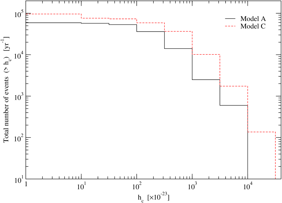
Figure 6: Distribution of dimensionless strain amplitudes for events received from across all redshifts.

We have seen above that the strain amplitude is rather insensitive to the frequency of the waves emitted. The frequency does matter for LISA detections as its peak sensitivity lies in a rather narrow band around 0.01 Hz. Merging seed MBH binary systems have very low strain amplitudes, especially at high redshifts, but peak frequencies well above 1 Hz. The only way of detecting these is during a significantly earlier phase of their coalescence when their frequency is lower.

3 Gamma rays from MBH formation and merging

Another exciting possibility is that the more massive of the first stars forming at high redshift conclude their lives in hypernovae, which be visible as gamma-ray bursts (GRBs). GRBs should be detectable to high redshift by upcoming satellite missions, which would allow us to study events from the first era of star formation directly. In contrast to the other observations mentioned above, such observations cannot be used to verify the hierarchical MBH merging scenario. GRB observations might provide constraints on the abundance of the first massive stars, however, and in this way allow us to test this part of our model directly.

GRBs are the brightest explosive events in the Universe. Typically they involve the emission of large amounts of radiative energy, of the order $\sim 10^{52-54}$ ergs in $\gamma$ rays, over a period of only a few seconds. A GRB is followed by an afterglow in the X-ray, optical or radio parts of the spectrum and lasts from days to weeks. The total energy emitted in an afterglow is typically two or three orders of magnitude below that of the actual burst. Spectroscopy has been carried out on the afterglow emissions as well as the emission of what appear to be host galaxies of the GRBs, once the afterglow itself has faded away sufficiently. In this way it has been possible to constrain the redshift of a number of GRBs below $z<3$. If GRBs could be used as standard candles in a similar way as type Ia supernovae, this would facilitate their use to calibrate the GRB distance-luminosity relation. On this basis one could then determine the maximum redshifts at which GRBs could still be detected by present and future observing missions, such as with the BATSE detector on the Compton Gamma-Ray Observatory or the SWIFT satellite due to be launched late in 2003 [Lamb & Reichart 2000]. For a number of GRBs for which redshifts could be established, Lamb & Reichart (2000) found that SWIFT could have in principle detected these out to redshifts of $z\sim 20$, and some to $z\sim 70$. For further details of GRBs their afterglows the reader is referred to the review by Piran (2000) and the extensive work by Bloom (2002) and references therein. For the following we assume that GRBs are in principle detectable out to redshifts beyond $z>20$.

A range of processes have been discussed that could be the cause for GRBs. As mentioned, one of these is the possibility that GRBs are produced by the collapse of massive stars. In the following we exclusively focus on this possibility and attempt to estimate the number of GRBs from massive population III stars in our model.

3.1 Number of GRBs from massive star collapse

The procedure to compute the total number of GRBs across all relevant redshifts is very similar to the one we used to determine the gravitational wave events. It is different in that we only deal with the very first stars, and are not concerned with the subsequent merging of the MBHs these stars leave behind. This is therefore a purely analytical argument with no recourse to our simulation data concerning the merging and dynamical evolution of MBHs.

Again, we estimate the abundance of minihaloes at the redshifts in question ($z\sim 25$). Depending on how many massive stars form per halo, we can then determine the expected number of GRBs. A similar route has been followed in previous work. In this case the abundance of massive stars per halo/galaxy was assumed to trace the star formation rate at the respective redshift [Bromm & Loeb 2002, Roy Choudhury & Srianand 2002]. We assume that every minihalo between a maximum redshift $z_{max}$, corresponding to a $2.5$–$3.5\sigma$ peak, and a minimum redshift determined by the end of first star formation, which we take as $z_{min}\sim 20$, produces one star that explodes as a hypernova with an associated GRB.

We have seen that a hypernova leads to the expulsion of all gas from minihaloes. Each minihalo can thus only ever produce one GRB. This is a problem as we now require each halo to retain a memory of whether and when it produced a GRB. For this reason it is not strictly correct to use the Press-Schechter mass function to compute the number density of haloes at a given redshift and equate the result with the number density of GRBs. A halo more massive than $M_{min}$ may have already lost all its gas through a hypernova at some earlier stage when it was significantly less massive. In practice, however, the Press-Schechter approach is more than adequate for two reasons. First, the PS mass function is steepest for large masses corresponding to haloes collapsing from high peaks as is the case for all minihaloes in our redshift range. The number density of haloes with mass $M_{h}\geq M_{min}$ is therefore vastly dominated by haloes with masses very close to $M_{min}$. Secondly, the survival time for haloes collapsing from high peaks is very short [Lacey & Cole 1993]. That means that by far most haloes with $M_{h}\geq M_{min}$ will have formed at or very shortly before the redshift in question and the probability of previous star formation and a GRB is very small.

If we identify a GRB event with the collapse of a minihalo, the rate of GRBs at any given redshift is then approximately

$$\frac{{\rm~{}d}\nu_{GRB}}{{\rm~{}d}z}{\rm~{}d}z\approx 4\pi D(z)^{2}{\rm~{}d}D(z)\int_{M_{min}}^{\infty}\frac{{\rm~{}d}^{2}n_{h}}{{\rm~{}d}t~{}{\rm~{}d}M}{\rm~{}d}M$$ (26)

where we have used the rate of change of the minihalo mass function

$$\frac{{\rm~{}d}^{2}n_{h}}{{\rm~{}d}t~{}{\rm~{}d}M_{h}} = \left(\frac{2}{\pi}\right)^{1/2}\frac{\rho_{0}}{M_{h}^{2}}\left|\frac{{\rm~{}d}{~{}\rm ln}\sigma}{{\rm~{}d}{~{}\rm ln}M_{h}}\right|~{}u$$

$$\times~{}{~{}\rm exp}\left[{-\frac{1}{2}u^{2}}\right]\left[\frac{1}{u}\frac{{\rm~{}d}u}{{\rm~{}d}t}-u\frac{{\rm~{}d}u}{{\rm~{}d}t}\right]$$

$$= \frac{{\rm~{}d}n_{h}}{{\rm~{}d}M_{h}}\frac{{\rm~{}d}u}{{\rm~{}d}t}\left[\frac{1}{u}-u\right]$$

and $u=\delta_{c}/[\sigma(M_{h})*D_{grow}(t)]$. We have shown the mass function and its rate of change in figure 7.

Figure 7: Top: Redshift dependent comoving number density of haloes with mass $M_{h}>M_{min}$. From top to bottom the curves correspond to a $M_{min}=\{1,3,10\}\times 10^{5}M_{\odot}h^{-1}$. Bottom: Rate of change of minihalo number density. The curves are in the same order.

3.2 Rate of GRBs received

For GRBs at the very high redshifts we are considering, no afterglow emission can be detected anymore. An accurate redshift determination is thus not possible unless a unique distance-luminosity relation for GRBs could really be established. If all GRBs do have the same total luminosity and peak photon flux, we have a unique distance-luminosity relation and thus a unique redshift-luminosity relation. Eqn. (3.1) above can then be converted into a flux distribution $F_{GRB}(z)$ using ${\rm~{}d}z\propto-2\pi D(z)^{3}/(10^{52-54}~{}{\rm erg})({\rm~{}d}D/{\rm~{}d}z)^{-1}{\rm~{}d}F_{GRB}$.

However, the case for a unique GRB distance-luminosity relation has yet to be made. To test our model we therefore focus on a prediction of the rate of GRBs to be compared with those detected by e.g. the SWIFT mission. We integrate eq. (3.1) over the redshift range of population III star formation to arrive at the total rate of GRBs received.

$$\nu_{GRB,rec}=\int_{z_{max}}^{z_{min}}(1+z)^{-1}\frac{{\rm~{}d}\nu_{GRB}}{{\rm~{}d}z}{\rm~{}d}z$$ (28)

Figure 8: Number of GRB events received per year originating from redshift $z$ to $z+{\rm~{}d}z$. The dashed curve shows the total number of GRB events from $z\geq 20$. From top to bottom the curves correspond to a $M_{min}=\{1,3,10\}\times 10^{5}M_{\odot}h^{-1}$.

This is shown in figure 8, together with rate of GRB events originating from any given redshift interval for three different values of $M_{min}$, assumed constant over the redshift range $20<z<30$. We find that the total number of GRB events received per year from this redshift range varies between $\nu_{GRB}\approx 3\times 10^{6}-2\times 10^{5}{\rm yr}^{-1}$ for $M_{min}=10^{5}$ to $10^{6}$ ${\rm M}_{\odot}$ respectively. Even for $M_{min}=3\times 10^{5}$ ${\rm M}_{\odot}$ at $z=25$, it may still make more sense to consider a larger halo mass, since by definition baryons – and therefore stars – in minihaloes only cool on a Hubble timescale, whereas we have assumed that GRB events coincide with the collapse of the haloes within which they occur. At $z=25$, for instance, a halo mass three times larger than the minihalo mass we used would result in a cooling time that is about a tenth of the Hubble time at that redshift and so more in line with this assumption.

A conservative estimate for the total number of GRB events received is $\nu_{GRB}\approx 2\times 10^{5}{\rm yr}^{-1}$, assuming that halo collapse, star formation and GRB coincide and that first star formation ends at $z=20$. How many of these could actually be observed depends on whether or not GRBs are luminous enough to still be detected at these distances.

3.3 Gamma rays from MBH mergers

If a small fraction of the gravitational energy from MBH mergers is released in the form of gamma rays - maybe due to the fast accretion of large amounts of material in the very close vicinity of the MBHs - we may be able to see these. For an inspiralling MBH binary the energy radiated away in gravitational waves, $L_{gw}$ is [Shapiro & Teukolsky 1983]

$$L_{gw} = \frac{32}{5}\frac{G^{4}}{c^{5}}\frac{M_{12}^{3}~{}\mu_{12}^{2}}{a_{0}^{5}}$$ (29)

$$= 5.43\times 10^{40}\left(\frac{a_{0}}{10^{8}{~{}\rm m}}\right)^{-5}\left(\frac{M_{12}}{10^{3}~{}{\rm M}_{\odot}}\right)^{3}$$

$$\times\left(\frac{\mu_{12}}{10^{3}~{}{\rm M}_{\odot}}\right)^{2}~{}{\rm erg~{}s}^{-1}$$

and combining this with the characteristic merger time scale eq 8 this becomes

$$L_{gw} = 2.13\times 10^{50}\left(\frac{\tau_{0}}{{\rm s}}\right)^{-5/4}\left(\frac{M_{12}}{10^{3}~{}{\rm M}_{\odot}}\right)^{1/2}$$ (30)

$$\times\left(\frac{\mu_{12}}{10^{3}~{}{\rm M}_{\odot}}\right)^{3/4}~{}{\rm erg~{}s}^{-1}$$

If we now multiply this with $1/f_{max}$ (eq 7) we can estimate the energy radiated away on the last orbit before final coalescence.

$$L_{gw}\approx 3\times 10^{50}\left(\frac{M_{12}}{10^{3}~{}{\rm M}_{\odot}}\right)^{1/4}\left(\frac{\mu_{12}}{10^{3}~{}{\rm M}_{\odot}}\right)^{3/4}~{}{\rm erg}$$ (31)

It is interesting to compare this with GRBs. A typical GRB lasts between a fraction of a second to minutes and emits total energies between $10^{51}-10^{54}$ erg [Piran 2000] and about a factor 100 less if we assume beamed emission. As far as the duration of GRBs is concerned this is matched by the period of the last orbits of MBH binaries with mass $M_{12}\sim 1000$ ${\rm M}_{\odot}$($\tau_{0}=1/f_{max}\sim 0.1$ seconds) to $M_{12}\sim 10^{6}$ ${\rm M}_{\odot}$($\tau_{0}\sim 100$ seconds). This means that if some fraction $\epsilon_{\gamma}\mathrel{\hbox{\hbox to0.0pt{\hbox{\lower 4.0pt\hbox{$\sim$}}\hss}\hbox{$>$}}}3\times 10^{-2}$ of gravitational wave energy is emitted in gamma rays, merging MBHs could account for some beamed GRBs. At the lower end the detection limit of the BATSE instrument on the Compton Gamma Ray Observatory implies $\epsilon_{\gamma}\mathrel{\hbox{\hbox to0.0pt{\hbox{\lower 4.0pt\hbox{$\sim$}}\hss}\hbox{$>$}}}10^{-6}$ for MBH mergers to be detected out to cosmological distances. For isotropically emitting GRBs $\epsilon_{\gamma}$ would need to be a factor 100 or so higher.

4 Summary and Conclusions

In this paper we were mainly concerned with probing our model at high redshifts. The merging of MBHs in the context of the hierarchical merging of galaxies and haloes would lead to the emission of gravitational waves, that could be detected with the LISA mission due to be launched in the next decade. We can draw the following conclusions:

• The merger rate per unit redshift peaks at $z\sim 4$–$6$. The peak shifts to lower redshifts if events with higher dimensionless strain amplitudes are considered.

• The predicted merger events all have strain amplitudes above $h_{c}>10^{-23}$, and most above $10^{-22}$, so that LISA should be able to detect most of these.

• The total number of MBH merger events received are about $10^{4}$–$10^{5}$ per year. This is at least an order of magnitude larger than typical estimates for (‘major’) mergers of SMBHs in hierarchical structure formation scenarios. Our larger number arises from the inclusion of a lot of mergers with fairly large binary mass ratios, i.e. what we may qualify as ‘minor’ mergers. The required population of MBHs are the (merged) remnants of the first massive stars in the universe. An estimate of this population was the subject of paper I in this series.

• In contrast to previous analytical work our predictions are based on a more accurate and explicit modelling of the dynamical evolution of MBHs in galactic haloes. This has allowed us to follow MBH merging in haloes at higher redshift and therefore also down to lower precursor masses.

• If the collapse of the first massive population III stars into MBHs is accompanied by gamma-ray bursts (GRBs), these might allow us to probe the abundance of the first stars as well as their spatial distribution. We predict $10^{5}$–$10^{6}$ GRBs per year originating at redshifts higher than 20, if there is one massive star per star-forming minihalo associated with a GRB.

• A fraction of the gravitational wave energy in MBH mergers may be released in gamma rays, e.g. through interaction with remnant gas in the close vicinity of the coalescing binary. If GRB emissions are beamed this fraction must be $\epsilon_{\gamma}>10^{-6}$ for the resulting bursts of gamma rays to be detectable at cosmological distances and $\epsilon_{\gamma}>3\times 10^{-2}$ to possibly account for some of the proper GRBs. However, the short event duration makes it difficult to identify them unless a GRB style after-glow is associated with them.

While the prediction of gravitational wave events and GRBs both depend sensitively on the initial assumption of massive star formation, the additional assumptions of efficient merging for gravitational waves and that GRBs are created in the process of massive star collapse, further increase uncertainty. All these assumptions are in principle verifiable primarily with improved numerical simulations (The role of gas in BH binary mergers, improved resolution in star formation and collapse simulations in a cosmological context). For the time being, the prediction of event rates of 10 to 100 a day should provide motivation to look out for them in present and upcoming observations. Qualitatively the most important thing is to note, that we could potentially observe the highly energetic events accompanying both the formation (via GRBs) and merger (by gravity waves) of MBHs, and therefore probe the high redshift regime.

References

- [Abel, Bryan & Norman 2000] Abel T., Bryan G.L., Norman M.L., 2000, ApJ, 540, 39
- [Armitage & Natarajan 2002] Armitage P.J., Natarajan P., 2002, ApJ, 567, L9
- [Barnes 2002] Barnes J.E., 2002, MNRAS, 333, 481
- [Barnes & Hernquist 1996] Barnes J.E., Hernquist L., 1996, ApJ, 471, 115
- [Begelman, Blandford & Rees 1980] Begelman M.C., Blandford R.D., Rees M.J., 1980, Nature, 287, 307
- [Binney & Tremaine 1987] Binney J., Tremaine S., 1987, Galactic Dynamics. Princeton Univ. Press, Princeton
- [Bloom 2002] Bloom J.S., PhD Thesis, CalTech 2002
- [Bromm, Coppi & Larson 2002] Bromm V., Coppi P.S., Larson R.B., 2002, ApJ, 564, 23
- [Bromm & Loeb 2002] Bromm V., Loeb A., 2002, ApJ, 575, 111
- [Colpi, Mayer & Governato 1999] Colpi M., Mayer L., Governato F., 1999, ApJ, 525, 720
- [de Araujo, Miranda & Aguiar 2002] de Araujo J.C.N., Miranda O.D. & Aguiar O.D., 2002, MNRAS, 330, 651
- [Escala et al. ] Escala A, Larson R.B., Coppi P.S., Mardones D., 2004, ApJ, 607, 765
- [Ferrarese 2002] Ferrarese L., 2002, ApJ, 578, 90
- [Flanagan & Hughes 1998] Flanagan É.É., Hughes S.A., 1998, Phys. Rev. D57,8
- [Fuller & Couchman 2000] Fuller T.M., Couchman H.M.P., 2000, ApJ, 544, 6
- [Haehnelt 1994] Haehnelt M., 1994, MNRAS, 269, 199
- [Heger et al. 2002] Heger A., Woosley S., Baraffe I., Abel T. 2002, in Proc. MPA/ESO, Lighthouses of the Universe: The Most Luminous Celestial Objects and Their Use for Cosmology. ESO, Garching, p. 369
- [Hutchings et al. 2002] Hutchings R.M., Santoro F., Thomas P.A., Couchman H.M.P., 2002, MNRAS, 330, 927
- [Islam, Taylor & Silk 2003, herafter paper I] Islam R.R., Taylor J.E., Silk J., MNRAS submitted, astro-ph/0307171
- [Islam, Taylor & Silk 2003, herafter paper II] Islam R.R., Taylor J.E., Silk J., MNRAS submitted, astro-ph/0309558
- [Lacey & Cole 1993] Lacey C., Cole S., 1993, MNRAS, 262, 627
- [Lamb & Reichart 2000] Lamb D.Q., Reichart D.E., 2000, ApJ, 536, 1
- [Menou, Haiman & Narayanan 2001] Menou K., Haiman Z., Narayanan V.K., 2001, ApJ, 558, 535
- [Milosavljevi c & Merritt 2001] Milosavljevi c M., Merritt D., 2001, ApJ, 563, 34
- [Misner, Thorne & Wheeler 1973] Misner C.W, Thorne K.S. & Wheeler J.A., 1973, Gravitation. W.H. Freeman and Co., San Francisco, p.988
- [Naab & Burkert 2001] Naab T., Burkert A., 2001, ASP Conf. Ser. 249: The Central Kiloparsec of Starbursts and AGN: The La Palma Connection, p. 735
- [Nakamura et al. 1997] Nakamura T., Sasaki M., Tanaka T., Thirne K.S., 1997, ApJ, 487, L139
- [Omukai & Palla 2001] Omukai K., Palla F., 2001, ApJ, 561, L55
- [Peters 1964] Peters P.C., 1964, Phys. Rev. B136,1224
- [Piran 2000] Piran T., 2000, Phys. Rep., 333, 529
- [Quinlan 1996] Quinlan G.D., 1996, NewA, 1, 35
- [Roy Choudhury & Srianand 2002] Roy Choudhury T., Srianand R., 2002, MNRAS, 336, L27
- [Schneider et al. 2000] Schneider R., Ferrara A., Ciardi B., Ferrari V. et al. , 2000, MNRAS, 317, 385
- [Shapiro & Teukolsky 1983] Shapiro S.L. & Teukolsky S.A., 1983, Black Holes, White Dwarfs and Neutron Stars. Wiley-Interscience, New York
- [Taylor & Babul 2004] Taylor J.E., Babul A., 2004, MNRAS, 348, 811
- [Tegmark et al. 1997] Tegmark, M., Silk, J., Rees, M. J., Blanchard, A., Abel, T., & Palla, F., 1997, ApJ, 474, 1
- [Thorne 1989] Thorne K. S., 1989, in Hawking S.W, Israel W., eds, Three Hundred Years of Gravitation, Cambridge Univ. Press, Cambridge, p. 330
- [Volonteri, Haardt & Madau 2003] Volonteri M., Haardt F., Madau. P, 2003, ApJ, 582, 559
- [Yu 2002] Yu Q., 2002, MNRAS, 331, 935