Reconstruction of solar activity for the last millennium using ¹⁰Be data

In a recent paper (Usoskin et al., 2002a), we have reconstructed the concentration of the cosmogenic ¹⁰Be isotope in ice cores from the measured sunspot numbers by using physical models for ¹⁰Be production in the Earth’s atmosphere, cosmic ray transport in the heliosphere, and evolution of the Sun’s open magnetic flux. Here we take the opposite route: starting from the ¹⁰Be concentration measured in ice cores from Antarctica and Greenland, we invert the models in order to reconstruct the 11-year averaged sunspot numbers since 850 AD. The inversion method is validated by comparing the reconstructed sunspot numbers with the directly observed sunspot record since 1610. The reconstructed sunspot record exhibits a prominent period of about 600 years, in agreement with earlier observations based on cosmogenic isotopes. Also, there is evidence for the century scale Gleissberg cycle and a number of shorter quasi-periodicities whose periods seem to fluctuate in the millennium time scale. This invalidates the earlier extrapolation of multi-harmonic representation of sunspot activity over extended time intervals.

1 Introduction

Sunspot numbers (SN) form the most common index of solar activity reflecting the varying strength of the hydromagnetic dynamo process which generates the solar magnetic field.

There are two approaches to reconstruct SN for times prior to regular direct observations. The first approach is based on mathematical extrapolation using the statistical properties of the SN record observed during the last 300 years. Such models provide, e.g., a single (11.1-year) carrier frequency or a multi-harmonic representation of the measured SN, which is then extrapolated backward in time (Schove (1955); Nagovitsyn (1997); Rigozo et al. (2001)). Some models also use fragmentary data from naked-eye sunspot observations or sightings of aurorae. The disadvantage of this approach is that it is not a reconstruction based upon a description of physical processes but rather a prediction based on extrapolation. Clearly such models cannot include periods exceeding the time span of observations upon which the extrapolation is based. Hence, the pre- or post-diction becomes increasingly unreliable with extrapolation time and its accuracy is hard to estimate.

The second approach is based on measured archival proxies of SN such as cosmogenic isotopes (see, e.g. ; Lingenfelter (1963); Beer et al. (1990); O’Brien et al. (1991); Damon & Sonett (1991); Beer (2000)). While this approach is based upon real measurements, the quantitative relationship between SN and the measured cosmogenic isotope concentration is usually described in an ad-hoc fashion by a simple inverse relation.

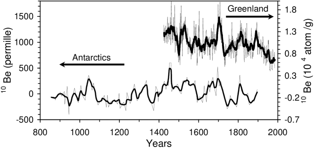
Figure 1: Raw and smoothed ¹⁰Be data. The lower curves (left axis) give the raw (thin curve) and the 1-2-1 filtered 8-year-averaged data from Antarctica (Bard et al. (1997)). The upper curves (right axis) show the raw and the 11-year smoothed yearly data from Greenland (Beer et al. (1990)).

In this paper we follow an improved version of the second approach and reconstruct the SN for the last millenium using a physical model with a realistic relation between the concentration of the cosmogenic ¹⁰Be isotope in polar ice and the SN. The ¹⁰Be concentration corresponds well, with a response time of 1-2 years, to the flux of primary cosmic rays in the vicinity of the Earth (Bard et al. (1997); Beer (2000)). We use two sets of ¹⁰Be data shown in Fig. 1. One is the annual series of ¹⁰Be concentration in Greenland ice (Dye-3 site, 65.15 N 43.82 W) for the years 1424–1985 (Beer et al. (1990)). The other series gives the ¹⁰Be concentration with roughly 8-year averaging in Antarctic ice (South Pole) for the years 850–1900 (Raisbeck et al. (1990); Bard et al. (1997)).

2 Model

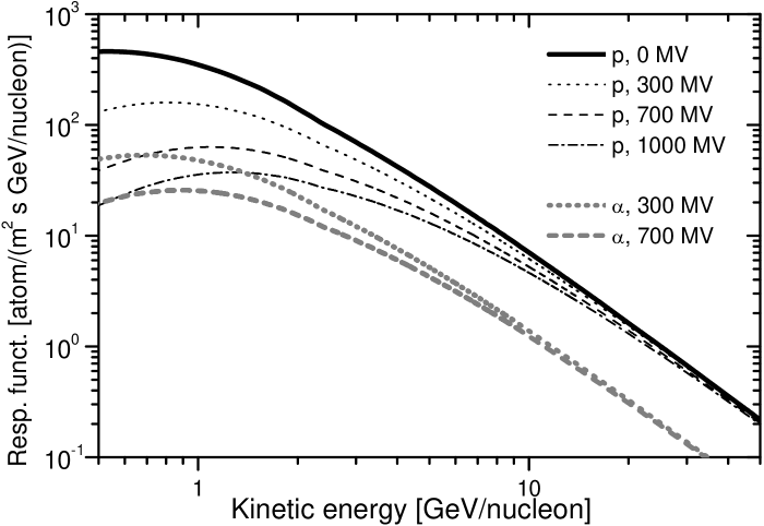
Figure 2: The differential response function of ¹⁰Be to the two main species of galactic cosmic rays, protons and $\alpha-$particles, for different values of the heliospheric modulation strength, $\Phi$.

In a recent paper (Usoskin et al. 2002a ), we have developed a model which connects the sunspot number $N$ with the cosmic ray flux (CR) through the source term, $S$, the open solar magnetic flux, $F_{o}$, and the modulation strength, $\Phi$, through a sequence of steps:

$$N\stackrel{{\scriptstyle(1)}}{{\longrightarrow}}S\stackrel{{\scriptstyle(2)}}{{\longrightarrow}}F_{o}\stackrel{{\scriptstyle(3)}}{{\longrightarrow}}\Phi\stackrel{{\scriptstyle(4)}}{{\longrightarrow}}CR\stackrel{{\scriptstyle(5)}}{{\longrightarrow}}\,^{10}{\rm Be}$$ (1)

Steps (1) and (2) are based upon a model for the open solar magnetic flux (Solanki et al. (2000)), steps (3) and (4) on a 1D model of heliospheric transport of CR (Usoskin et al. 2002b ). For step (5) we have earlier (Usoskin et al. 2002a ) assumed that the ¹⁰Be production and the related concentration in polar ice is proportional to the flux of CR with an energy of about 2 GeV. Here we calculate step (5) using a more realistic production rate of ¹⁰Be by CR in the Earth’s atmosphere. The local ¹⁰Be production rate, $R$, is given by

$$R=\int_{P_{c}}^{\infty}X(P)\cdot Y(P)dP,$$ (2)

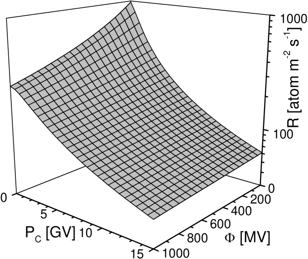
Figure 3: Production rate of ¹⁰Be in the atmosphere as a function of the heliospheric modulation strength, $\Phi$, and the local rigidity cutoff, $P_{c}$.

where $P_{c}$, $X(P)$, $Y(P)$, and $P$ are the local rigidity cutoff, the differential CR spectrum near the Earth, the differential yield function of ¹⁰Be production, and the primary CR particle’s rigidity, respectively.

Heavier species (mostly $\alpha-$particles) compose a part of all CR, about 6% in particle number or about 25% in nucleon number according to recent high-precision measurements (see, e.g. ; Boenzio et al. (1999); Alcaraz et al. 2000a ; Alcaraz et al. 2000b ). Moreover, since heavier nuclei are less modulated in the heliosphere than protons, their contribution is larger at lower energies (about 1–2 GeV/nucleon) which are most effective for ¹⁰Be production in the atmosphere. Therefore, we have taken $\alpha-$particles into account in the present study. Species heavier than $\alpha-$particles can be neglected because of their low abundance in CR).

Using differential CR (protons and $\alpha-$particles) spectra obtained from our heliospheric model (Usoskin et al. 2002b ), and the differential yield function of ¹⁰Be production in the atmosphere (Webber & Higbie (2003)), we have calculated the ¹⁰Be differential response function (Fig. 2) which is the integrand appearing in Eq. (2). One can see that the contribution of heavier nuclei to ¹⁰Be production becomes significant at energies lower than 2 GeV/nucleon, while the overall production rate $R$ is mostly determined by protons. The mean energy for ¹⁰Be production move in the course of a solar activity cycle, varying between 1.5 GeV ($\Phi$=300 MV corresponding to recent solar cycle minima) and 4 GeV ($\Phi$=1000 MV corresponding to solar cycle maxima), which is somewhat larger than the value of 2 GeV used earlier (McCracken & McDonald (2001); Usoskin et al. 2002a ). This results from the fact that the magnitude of the solar cycle modulation of CR greatly increases towards lower energies, which decreases the effective energy responsible for the ¹⁰Be variations with respect to the mean energy. The total ¹⁰Be production rate is shown in Fig. 3 as a function of the heliospheric modulation strength, $\Phi$, and $P_{c}$. The resulting ¹⁰Be concentration in polar ice is assumed to be proportional to the ¹⁰Be production rate, i.e., we ignore the details of the atmospheric transport and deposition of ¹⁰Be (Masarik & Beer (1999)) since we are interested in much longer time scales.

We now invert the model by going through the sequence of Eq. (1) in reverse order:

$$N\stackrel{{\scriptstyle(1^{\prime})}}{{\longleftarrow}}S\stackrel{{\scriptstyle(2^{\prime})}}{{\longleftarrow}}F_{o}\stackrel{{\scriptstyle(3^{\prime})}}{{\longleftarrow}}\Phi\left(\stackrel{{\scriptstyle(4^{\prime})}}{{\longleftarrow}}CR\stackrel{{\scriptstyle(5^{\prime})}}{{\longleftarrow}}\right)\,^{10}{\rm Be}$$ (3)

Steps ($5^{\prime}$) and ($4^{\prime}$) are taken in one stride so that from a measured ¹⁰Be concentration in polar ice at a given location (given $P_{c}$), we determine the corresponding heliospheric modulation strength, $\Phi$, using the relationship shown in Fig. 3. Steps ($1^{\prime}$)-($3^{\prime}$) are inversions of the corresponding steps (1)-(3) in the direct model. In step ($3^{\prime}$), a power-law relation between $\Phi$ and the open magnetic flux, $F_{o}$, is used (Usoskin et al. 2002a ):

$$F_{o}=0.023\ \Phi^{0.9},$$ (4)

where $\Phi$ and $F_{o}$ are given in MV and $10^{14}\ {\rm Wb}$, respectively.

In step ($2^{\prime}$) we invert the following equation which connects the evolution of the open magnetic flux $F_{o}$ with the source function $S$ (Solanki et al. (2000)),

$${dF_{o}\over dt}=S-{F_{o}\over\tau},$$ (5)

where $\tau=4\,$yr represents the characteristic decay time. This equation includes differentiation, and when employing it to compute $S$ from $F_{o}$, its inversion is stable only for smooth (noiseless) data series, for which the time derivative does not fluctuate strongly from one data point to the next.

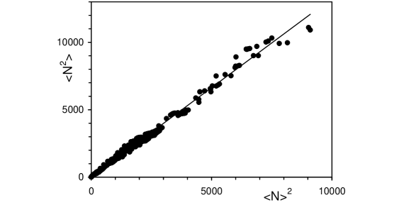
Figure 4: Scatter plot of 11-year averaged $\langle N^{2}\rangle$ vs. $\langle N\rangle^{2}$ based upon the yearly group sunspot numbers for 1700–2000. The regression line has a slope of $1.32\pm 0.01$.

Real ¹⁰Be data are noisy and do not fulfill these conditions (see Fig. 1). Therefore, a reconstruction of yearly SN values from the yearly sampled Dye-3 Greenland ¹⁰Be record is extremely noisy. However, averaging the yearly Greenland data by an 11-year running mean prior to reconstruction greatly reduces the noise and increases the stability of the procedure, although at the cost of losing information on variations shorter than a solar cycle. Similarly, a direct reconstruction using the 8-year-sampled South Pole record is also somewhat noisy. We therefore smooth the Antarctic data set using a 1-2-1 filter, which roughly corresponds to an 11-year smoothing. In what follows we only consider the (effectively 11-year) averaged data series, so that Eq. (5) takes the form

$$\langle{dF_{o}\over dt}\rangle=\langle S\rangle-\frac{\langle{F_{o}}\rangle}{\tau}\ ,$$ (6)

where the angular brackets indicate temporal averages. From the time sequence of averaged measured ¹⁰Be data we determine through steps ($3^{\prime}$)-($5^{\prime}$) the open flux values, $\langle{F_{o}}\rangle$. The corresponding values of the average source function, $\langle{S}\rangle$, are obtained by replacing the time derivative in Eq. (6) by a simple first-order finite difference.

The source function, $S$, is the following function of the sunspot number $N$

$$S(N)=\alpha\left(24.35+22N-0.061N^{2}\right)\,,$$ (7)

where $\alpha=1.95\cdot 10^{11}$ Wb/yr (Solanki et al. (2000)). In order to obtain the average sunspot number, $\langle{N}\rangle$, we have to to invert the time-averaged Eq.(7) and to express $\langle N^{2}\rangle$ in terms of $\langle N\rangle$. Unfortunately, there is no unique solution to this problem. A regression analysis based upon the 11-year-averaged group sunspot number (GSN) record (Hoyt & Schatten (1998)) since 1700 leads to a factor $1.32\pm 0.01$ (Fig. 4). Therefore, we have used the relation $\langle N^{2}\rangle=1.32\langle N\rangle^{2}$ in the inversion of Eq.( 7).

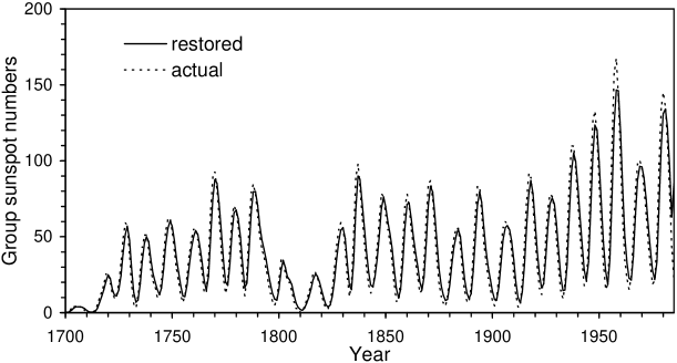
Figure 5: Actual and restored yearly group sunspot numbers for 1700–1985 as a test of the consistency of the inversion model.

In order to check the consistency of the full inversion procedure we have performed the following test. Using the direct model (Eq. 1), we calculated, similar to (Usoskin et al. 2002a ) but with the more realistic ¹⁰Be production described above, the expected ¹⁰Be concentration from the actual yearly group sunspot data (Hoyt & Schatten (1998)). The calculated ¹⁰Be concentration was then used as an input for the inversion (Eq. 3), from which the corresponding restored group sunspot numbers were determined. The result is shown in Fig. 5. Since the restored SN series is very close to the actual record (the RMS errors are $10.4$ for the yearly and $2.4$ for the 11-year averaged series), we conclude that the inversion procedure is consistent. We emphasize that a nearly perfect reconstruction such as that in Fig. 5 is only possible for almost ideal data, with little noise, good sampling, etc. The measured ¹⁰Be data do not fulfill these conditions nearly as well as the artificial record ¹⁰Be constructed from GSN, as discussed above.

3 Reconstruction of sunspot numbers

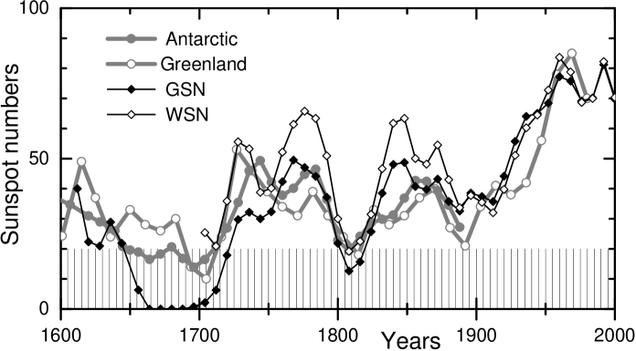
Figure 6: 11-year averaged sunspot numbers for the last 400 years: group sunspot numbers (GSN), Wolf sunspot numbers (WSN), SN reconstructed from Greenland ¹⁰Be and SN reconstructed from 1-2-1 filtered Antarctic ¹⁰Be data. The shaded area roughly indicates the range of averaged SN for which the model is less reliable.

As a first step, we have reconstructed the sunspot activity for the last 400 years from ¹⁰Be data using the model described above. Since direct sunspot observations exist for this period, we can compare the reconstructed and measured SN. The SN reconstructed from the two ¹⁰Be series are shown in Fig. 6, together with the measured Wolf and group sunspot numbers. The agreement between the reconstructed SN series based on the 11-year averaged Greenland ¹⁰Be and the measured SN is quite good for the period 1700–1985, with an RMS discrepancy of 11 (the cross-correlation is $r=0.78^{+0.06}_{-0.10}$) for GSN and 12.5 ($r=0.74^{+0.07}_{-0.12}$) for the Wolf sunspot series. The RMS deviation is 10 between the 1-2-1 filtered 8-year averaged GSN and SN reconstructed from the Antarctic ¹⁰Be series for 1700–1900 ($r=0.76^{+0.07}_{-0.12})$.

We note that the overall agreement between the reconstructed and measured SN is somewhat better for the group sunspot series than for the Wolf series. For example, in 1770–1800 and 1830–1880, the reconstructed SN is very close to the GSN while the WSN is systematically higher. The only exception is the period 1700–1750 when the reconstructed SN shows good agreement with the Wolf series while GSN is systematically lower (Fig. 6). This might imply that the group sunspot number values are somewhat too small during the first half of the $18^{th}$ century, in general agreement with the results of Letfus (2000). We note that the two reconstructed SN series lie closer together than the GSN and WSN series in the common time interval, i.e., between 1700 and 1900.

In summary, we conclude that our method reconstructs the measured sunspot numbers reasonably well for the last 400 years. The only exception is the Maunder minimum. Whereas the actual sunspot number is close to zero (Eddy (1976); Ribes & Nesme-Ribes (1993); Usoskin et al. (2000)) during this period, the reconstruction returns values between 10 and 25. This is due to the fact that the model is not reliable during extended periods of very low solar activity, as was already pointed out (Usoskin et al. 2002a ). On the other hand, the SN is still well reconstructed during the Dalton minimum circa 1800. Accordingly, we estimate that the reconstructed sunspot values are unreliable (overestimated) when SN$\leq 20$.

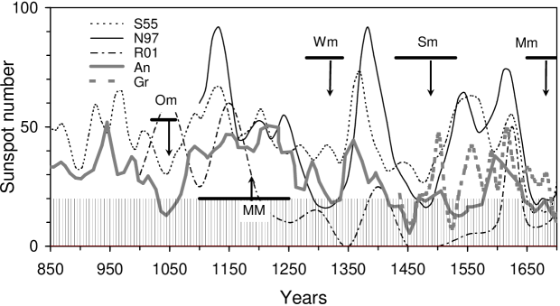
Figure 7: Sunspot activity (11-year averaged) during the pre-instrumental era: earlier extrapolations by Schove (1955 - S55), Nagovitsyn (1997 - N97) and Rigozo et al. (2001 - R01), and our SN reconstructions from 1-2-1 filtered 8-year Antarctic (An) and from 11-year averaged Greenland (Gr) ¹⁰Be series. The shaded area indicates the range of averaged SN for which the applicability of the model is limited. Horizontal bars with arrows denote the known grand minima and maxima: Maunder minimum (Mm), Spörer minimum (Sm), Wolf minimum (Wm), Oort minimum (Om) and the Medieval maximum (MM).

In the next step, we have reconstructed the SN in the millennium time scale (Fig. 7) using both the Greenland (since 1424) and the Antarctic (since 850) ¹⁰Be time series. Great minima as deduced from proxies like ¹⁴C, ¹⁰Be, etc., also appear in our reconstruction, as does the Medieval maximum (Stuiver & Braziunas (1989)). We note that, because of the above-mentioned limitations of our model, the reconstructed SN, although significantly reduced during great minima, never reach zero. While the SN reconstructions based upon the Antarctic and the Greenland data are rather consistent with each other after 1600 (Fig. 6), they exhibit notable differences in 1480–1600. The Antarctic series shows an extended minimum while the Greenland series exhibits pronounced maxima in 1500 and in 1560. Since this interval corresponds to the Little Ice Age, climatic differences between Greenland and Antarctica may well be the source.

Fig. 7 also shows that for the pre-instrumental era before 1600 our reconstruction differs significantly from earlier results obtained by extrapolating multiharmonic representations of the measured SN (Schove (1955); Nagovitsyn (1997); Rigozo et al. (2001) - henceforth referred to as S55, N97 and R01, respectively). For example, the S55 and N97 series exhibit high maxima of activity around 1100, 1400 and 1550–1600, which are either not present or significantly lower in our reconstruction. On the other hand, R01 predicts a high maximum around 1050 when the Oort minimum, visible in all other series, is expected. Throughout the whole period covered by Fig. 7, our reconstruction shows much smaller variations of the SN level than the earlier series.

4 Periodic features

As discussed above, our reconstruction recovers the great minima and maxima of solar activity, which have been qualitatively deduced earlier. We now analyze the periodic features of the reconstructed SN series. Since we deal with either 11-year averaged or 1-2-1 filtered 8-year sampled series, we will discuss only periods longer than 40 years.

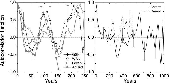
Figure 8: Autocorrelation function of the measured SN (group, GSN, and Wolf, WSN) and the reconstructed (from Greenland and Antarctic ¹⁰Be data) sunspot series. Left panel: autocorrelation function for the period 1700–2000 (1700–1900 for the Antarctic series; 1700–1985 for the Greenland series). Right panel: autocorrelation function for the period after 850 for the Antarctic series and after 1424 for the Greenland series. Error bars represent the 95% confidence interval.

First we compare the periodicities in the reconstructed series with those in the measured SN after 1700. In Fig. 8 (left panel) we plot the autocorrelation function (ACF) for this period for the two reconstructed and two measured SN series. The pattern is the same in all the four series, the main feature being a period of about 100 years, the Gleissberg secular cycle. One can see that all the curves are rather close to each other, within the 95% confidence interval, giving further support to the validity of our reconstruction method. The right panel of Fig. 8 shows the ACF for the last millennium for the reconstructions from the Greenland and Antarctic ¹⁰Be data. Two dominant periodicities are present in the reconstructed data. A cycle with an approximate period of 130 years is indicated by the consecutive peaks at 130, 260, 400, 530, …years in both SN series.

Moreover, a cycle with a period of about 600 years visible as a deep minimum with the lag of about 300 years in both series and as a maximum at 600–650 years in the Antarctic series.

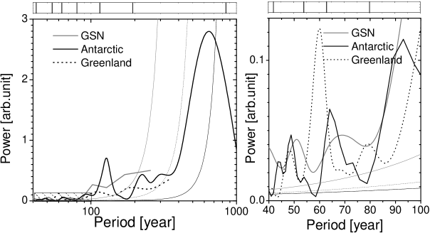
Figure 9: Power spectra of the sunspot number as reconstructed from the Antarctic (850–1900) and Greenland (1425–1980) ¹⁰Be series and of the group sunspot number (GSN) series (1700–2000). The right panel is a zoom of the hatched rectangle in the left panel. Thin lines indicate the corresponding 95 % confidence intervals. Bars in the upper panels represent the basic frequencies used by S55, N97 and R01 in their multi-harmonic models of sunspot activity.

Fig. 9 presents the power spectra of the two reconstructed SN series and the GSN series. The 95 % confidence levels of the power spectrum (Jenkins & Watts (1969)) are shown by thin lines. Note that the period after the Maunder minimum is too short to have a reliable power spectrum for the 8-year sampled Antarctic series, so that we have plotted the power spectrum using the whole data set. The power spectra for the GSN and for the Antarctic data are in a fair agreement in the period range from 40 to 100 years, revealing similar main periods: 52, 65–75 and 100 years in GSN series and 45–50, 65 and 90–95 years in the Antarctic series. The peak at 130 years, however, is not found in the GSN record. The power spectrum of the Greenland series (1425–1980) shows a very strong peak at 60 years which is absent in the other two series. Other significant peaks (50, 80 and 100–115 years) correspond roughly to similar peaks in both GSN and Antarctic power spectra. Periods longer than half of the analyzed interval cannot be reliably determined as shown by thin lines in Fig. 9. The power spectrum of the Antarctic series also exhibits a peak at about 220 years probably related to the so-called de Vries or Suess cycle, (Suess (1980); Wagner et al. (2001)) and a prominent peak close to 600 years (Sonett & Finney (1990)). The latter is in agreement with the autocorrelation function shown in Fig. 8. At the top of Fig. 9 the periods used by previous investigators to extrapolate the SN are marked. Not all of them agree with peaks in the power spectra of GSN and our reconstructions. We also note that periods of different quasi-periodicities (such as, e.g., the Gleissberg cycle) seem to be fluctuating on the long-time scale. This invalidates the earlier extrapolation of multi-harmonic representation of sunspot activity over extended time intervals.

5 Geomagnetic variations

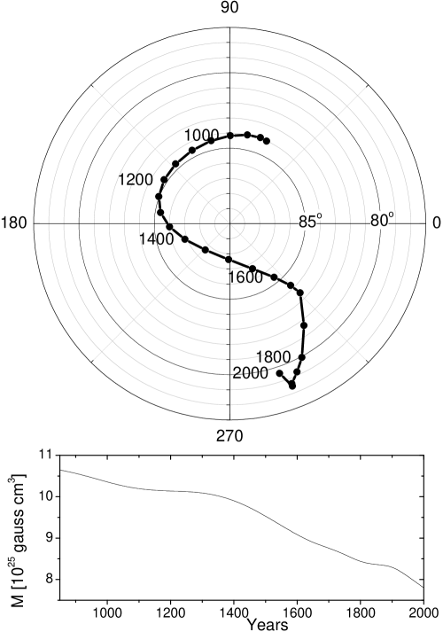
Figure 10: Variation of the parameters of the geomagnetic dipole during 850-2000 AD. Migration of the dipole axis (top panel, in geographical coordinates) and change of the virtual dipole moment $M$ (lower panel).

The above results were obtained assuming a local ¹⁰Be deposition and a constant rigidity cutoff of $P_{c}=0.5$ GV in Eq. (2), which roughly corresponds to the atmospheric cutoff. The geomagnetic field is known to change in time both in strength and orientation, which affects the ¹⁰Be production rate on time scales of centuries and longer (Baumgartner et al. (1998)). Fig. 10 shows the variation of the geomagnetic field for the period 850–2000 AD (see also Fig. 7 of Hongre et al. (1998)). The parameters of the geomagnetic field were taken from Hongre et al. (1998) for 850–1700 AD, from Bloxham & Jackson (1992) for 1700–1900, and from the IGRF (International Geomagnetic Reference Field) model for 1900–2000 AD. Using these data, we calculated the expected variation of the vertical geomagnetic cutoff, $P_{c}$, at the two ¹⁰Be sites using Størmer’s equation (Elsasser et al. (1956)):

$$P_{c}\propto M\cdot cos^{4}\Lambda,$$ (8)

where $M$ is the virtual dipole moment and $\Lambda$ is the local geomagnetic latitude. The calculated value of $P_{c}$ remains negligibly small (below 0.025 GV) for the South Pole during the whole interval studied here. The geomagnetic latitude of the South Pole site remains above $80^{\circ}$, i.e. inside the polar cap where geomagnetic field lines are open. Therefore, only the atmospheric cutoff was applied for the South Pole. The value of $P_{c}$ for the Dye-3 Greenland site remains below 0.5 GV during the period of available data (since 1424) and, therefore, can be neglected as well. At earlier times, however, the influence of the geomagnetic field becomes significant, e.g., the value of $P_{c}$ exceeds 1 GV for the Dye-3 site before the $14^{th}$ century.

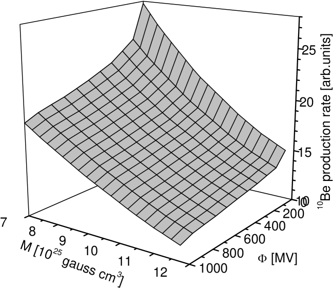
Figure 11: Global production rate of ¹⁰Be in the atmosphere as a function of the virtual geomagnetic dipole moment, $M$, and the modulation strength, $\Phi$.

We have also calculated the global ¹⁰Be production in the entire atmosphere as a function of the magnetic dipole moment and the modulation strength (Fig. 11, see also Fig. 2 in Beer (2000)). As an extreme case, we have performed a reconstruction of the SN assuming global mixing of ¹⁰Be before deposition, similar to ¹⁴C. The result is shown in Fig. 12 and is compared with the reconstruction based upon local ¹⁰Be deposition and the GSN record. Since the geomagnetic dipole was stronger in earlier times leading to a more effective shielding of the Earth, the same amount of globally distributed ¹⁰Be would require a stronger CR flux and, correspondingly, reduced sunspot activity. Therefore, the SN level corresponding to the global ¹⁰Be model is systematically below the local model and also the GSN level. This difference becomes increasingly larger for earlier times and the sunspot level goes systematically below 10 before 1600 in the global ¹⁰Be model. This implies that the local deposition model is closer to reality than global mixing, although the truth probably lies in between. Furthermore, the local ¹⁰Be model gives an upper limit to the level of sunspot activity since in the presence of atmospheric mixing the geomagnetic effects would require reduced activity levels at earlier times in order to retain consistency between the ¹⁰Be and GSN records.

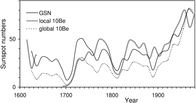
Figure 12: 11-year-averaged sunspot group sunspot number series (GSN) and the reconstructed SN for local and global ¹⁰Be deposition are represenetd by grey, solid, and dotted curves, respectively.

6 Conclusions

The sunspot number record is not only the most widely used proxy of solar activity, it is also one of the longest running scientific data series. Nonetheless, for many purposes it is still too short. For example, both the statistical investigation of the solar dynamo and studies of a possible influences of solar activity on climate would greatly profit from a longer time series.

Since direct observations are sparse and not very reliable before the era of telescopic observations we have used an indirect proxy, the concentration of the cosmogenic ¹⁰Be isotope in the ice sheets in Greenland and Antarctica. Unlike previous investigators, however, we have employed physical relations to convert the ¹⁰Be concentration into averaged sunspot numbers. A comparison of directly observed SN with the reconstructed values for the last 400 years confirms the reliability of the latter. To enhance the reliability over longer times we have also considered the possible influence of geomagnetic field variations. Taking the available data with a time resolution of the length of the solar cycle we have reconstructed the SN back to 850 AD.

We have also performed a detailed analysis of periodicities in the long-term solar activity record. Both applied methods, autocorrelation function and power spectrum, reveal that a number of strong periods in the directly measured sunspot series are also present in the SN record reconstructed for the same period of time. Some differences between records are found, but they are generally smaller than changes in dominant frequencies as different lengths of the time series are considered. In the higher frequency range, periods of about 50 and 65 years are visible in both measured and reconstructed series. The secular Gleissberg cycle, which is roughly 100 years in the GSN series, is split into the dominant 120–130-year and subdominant 90–95-year cycles in the reconstructed series, the latter being more prominent during the last 3–4 centuries. There is also evidence for an independent periodicity of about 220 years. This may be related to the de Vries (also called Suess) cycle, earlier known in, e.g., ¹⁴C isotope data. A strong cycle with a period of roughly 600 year is apparent in the reconstructed series based upon the Antarctic data. Both the GSN record and the the SN series reconstructed from the Greenland ¹⁰Be data are too short to exhibit this period, which is possibly related to the 650-year periodicity in the ¹⁴C data (Damon & Sonett (1991)).

In conclusion, we have presented here a new reconstruction of solar activity on the millennium time scale based upon a description of the related physical processes. The results will be the subject of further analysis.

- (1) Alcaraz, J., et al. (The AMS collaboration) 2000a, Phys. Lett. B, 490, 27.
- (2) Alcaraz, J., et al. (The AMS collaboration) 2000b, Phys. Lett. B, 494, 193.
- Bard et al. (1997) Bard, E., Raisbek, G.M., Yiou, F. & Jouzel, J. 1997, Earth and Planet. Sci. Lett., 150, 453.
- Baumgartner et al. (1998) Baumgartner, S., Beer, J., & Synal, H.A. 1998, Science 279, 1330.
- Beer et al. (1990) Beer, J., et al. 1990, Nature, 347, 164.
- Beer (2000) Beer, J. 2000, Space Sci. Rev., 93, 107.
- Bloxham & Jackson (1992) Bloxham, J., & Jackson, A., J. Geophys. Res., 97 (B13), 19537.
- Boenzio et al. (1999) Boenzio, M., et al. 1999, Astrophys. J., 518, 457.
- Damon & Sonett (1991) Damon, P.E., & Sonett, C.P. 1991 in: C.P. Sonnet, M.S. Giampapa, M.S. Matthews (eds.), The Sun in time, the University of Arizona, Tucson, 360.
- Eddy (1976) Eddy, J.A. 1976, Science, 192, 1189.
- Elsasser et al. (1956) Elsasser, W., Nay, E.P., & Winckler, J.R. 1956, Nature, 178, 1226.
- Hongre et al. (1998) Hongre, L., Hulot, G., & Khokhlov, A. 1998, Phys. Earth Planet. Inter., 106, 311.
- Hoyt & Schatten (1998) Hoyt D.V., & Schatten, K. 1998, Solar Phys. 179, 189.
- Jenkins & Watts (1969) Jenkins, G.M., & Watts, D.G. 1969, Spectral analysis and its applications, Holden-Day, San-Francisco.
- Letfus (2000) Letfus, V. 2000, Solar Phys., 194, 175.
- Lingenfelter (1963) Lingenfelter, R.E. 1963, Rev. Geophys., 1, 35.
- Masarik & Beer (1999) Masarik, J., & Beer, J. 1999, J. Geophys. Res., 104(D10), 12099.
- McCracken & McDonald (2001) McCracken, K.G., & McDonald, F.B. 2001, in :Proc. 27th Internat. Cosmic Ray Conf., Hamburg, 9, 3753.
- Nagovitsyn (1997) Nagovitsyn, Yu. A. 1997, Astron. Lett., 23, 742.
- O’Brien et al. (1991) O’Brien, K., De La Zerda Lerner, A., Shea, M.A., & Smart, D.F. 1991, in: C.P. Sonnet, M.S. Giampapa, M.S. Matthews (eds.), The Sun in time, the University of Arizona, Tucson, 317.
- Raisbeck et al. (1990) Raisbeck, G.M., Yiou, F.Y., Jouzel, J., & Petit, J.R. 1990, Phil. Trans. R. Soc. Lond., A330, 463.
- Ribes & Nesme-Ribes (1993) Ribes, J.C., & Nesme-Ribes, E. 1993, Astron.Astrophys., 276, 549.
- Rigozo et al. (2001) Rigozo, N.R., Echer, E., Vieira, L.E.A., & Nordemann, D.J.R. 2001, Solar Phys., 203, 179.
- Schove (1955) Schove, D.J. 1955, J.Geophys.Res., 60, 127.
- Solanki et al. (2000) Solanki, S. K., Schüssler, M., & Fligge, M. 2000, Nature, 408, 445.
- Sonett & Finney (1990) Sonett, C.P., & S.A. Finney 1990, Phil. Trans. R. Soc. Lond, A330, 413.
- Stuiver & Braziunas (1989) Stuiver, M., & Braziunas, T.F. 1989, Nature, 338, 405.
- Suess (1980) Suess, H.E. 1980, Radiocarbon, 22, 200.
- Usoskin et al. (2000) Usoskin, I.G., Mursula, K., & Kovaltsov, G.A. 2000, A&A, 354, L33.
- (30) Usoskin, I.G., Mursula, K., Solanki, S., Schüssler, M & Kovaltsov, G.A. 2002a, J. Geophys. Res., 107(A11), SSH 13-1, doi:10.1029/2002JA009343.
- (31) Usoskin, I.G., Alanko, K., Mursula, K., & Kovaltsov, G.A. 2002b, Solar Phys., 207, 389.
- Wagner et al. (2001) Wagner, G., et al., 2001, Geophys. Res. Lett., 28, 303.
- Webber & Higbie (2003) Webber, R., & Higbie, P.R. 2003, J. Geophys. Res., doi: 10.1029/2003JA009863, (in press).
- (34)