The cosmological evolution of metal enrichment in quasar host galaxies

Abstract

We study the gas metallicity of quasar hosts using cosmological hydrodynamic simulations of the $\Lambda$–cold dark matter model. Galaxy formation in the simulations is coupled with a prescription for black hole activity enabling us to study the evolution of the metal enrichment in quasar hosts and hence explore the relationship between star/spheroid formation and black hole growth/activity. In order to assess effects of numerical resolution, we compare simulations with different particle numbers and box sizes. We find a steep radial metallicity gradient in quasar host galaxies, with gas metallicities close to solar values in the outer parts but becoming supersolar in the center. The hosts of the rare bright quasars at $z\sim 5-6$ have star formation rates of several hundred $\hbox{$\rm\thinspace M_{\odot}$}{\rm\thinspace yr}^{-1}\,$ and halo masses of order $\sim 10^{12}\hbox{$\rm\thinspace M_{\odot}$}$. Already at these redshifts they have supersolar ($Z/Z_{\sun}\sim 2-3$) central metallicities, with a mild dependence of metallicity on luminosity, consistent with observed trends. The mean value of metallicity is sensitive to the assumed quasar lifetime, providing a useful new probe of this parameter. We find that lifetimes from $10^{7}-4\times 10^{7}\,{\rm yr}$ are favored by comparison to observational data. In both the models and observations, the rate of evolution of the mean quasar metallicity as a function of redshift is generally flat out to $z\sim 4-5$. Beyond the observed redshift range and out to redshift $z=6-8$, we predict a slow decline of the mean central metallicity towards solar and slightly subsolar values ($Z/Z_{\sun}\sim 0.4-1$), as we approach the epoch of the first significant star formation activity.

1. Introduction

The presence of supermassive black holes in the centers of nearby galaxies with a significant spheroidal component supports arguments that there is a fundamental link between the assembly of black holes and the formation of spheroids in galaxy halos. The evidence indicates that the mass of the central black hole is correlated with the bulge luminosity (e.g., Magorrian et al. 1998; Kormendy & Gebhardt 2001) and even more tightly with the velocity dispersion of its host bulge (Tremaine et al. 2002; Ferrarese & Merritt 2000; Merritt & Ferrarese 2001; Gebhardt et al. 2000), implying that the process that leads to the formation of galactic spheroids must be intimately linked to the growth of central supermassive black holes with commensurate mass.

Quasars at high redshift, the black hole remnants of which we find in galaxies today, provide us with a direct tool for investigating the relation between black hole and spheroidal formation. There are indications that high redshift quasar hosts are often strong sources of sub-mm dust emission (Omont et al. 2001; Cox et al. 2002; Carilli et al. 2000, 2002), suggesting that quasars were common in massive galaxies at a time when they were undergoing vigorous star formation. Metal abundance studies based on the gas of the broad line region (BLR) of quasars (e.g. Hamann & Ferland 1993; 1999; Hamann et al. 2002; Dietrich et al. 1999; 2003a,b and references therein) provide valuable information on the chemical enrichment of quasar host galaxies. In particular, these studies have shown that the interstellar medium of the quasar host galaxies has a metallicity which is typically super-solar with a mean value $Z\sim 4-5\,Z_{\sun}$, showing no evolution within the observed redshift range $3.5\leq z\leq 5$. In the context of galaxy evolution, this must mean that quasars mark the loci where massive galaxies are being assembled, undergoing significant star formation and building the central black holes.

Quasar metallicities offer us a potentially powerful probe of the Universe at redshifts beyond those at which objects have been detected so far. As pointed out by Dietrich and coauthors, the star formation timescales necessary to build up a reservoir of metal-rich gas by $z\sim 4-5$ indicate the presence of massive star formation already at $z\sim 6-10$. Other than the possible signature of reionization at $z\sim 17-20$ seen by the WMAP satellite (Kogut et al. 2003), information on the Universe at these epochs is difficult to obtain. By modeling the evolution of structure from these earliest times on it is, however, becoming possible to make quantitative predictions for quasar metallicities. The number density of rare luminous quasars is a stringent test of models (Efstathiou and Rees 1988), and their metallicities offer both a consistency test and a window on star formation at an epoch when the quasars were forming. Such measurements are complimentary to those of the metallicity of gas in the intergalactic medium from quasar absorption lines. The metallicity in the extreme environments close to the centers of hosts is also likely to be sensitive to events at earlier epochs, and can tell us about the timescales for the assembly of material in the galaxies themselves. The star formation rates required to produce metal-rich gas are sensitive to the structure of dark matter on small scales (see e.g. Yoshida et al.  2003a,b) as well as the parameters which govern the stellar mass function.

Several groups have discussed the link between cosmological evolution of QSOs and the formation history of galaxies (see e.g.; Monaco et al. 2000; Kauffmann & Haehnelt 2000; Ciotti & van Albada 2001; Wyithe & Loeb 2002; Granato et al. 2003; Haiman, Ciotti & Ostriker 2003 and references therein). Here we use cosmological hydrodynamical simulations coupled with a prescription for black hole activity in galaxies to follow the evolution of the metal enrichment in quasar host galaxies and therefore explore the relation between star/spheroid formation and black hole growth/activity. The simulations (Springel & Hernquist 2003a,b) include a novel prescription for star formation and feedback processes in the interstellar medium that is able to yield a numerically converged prediction for the full star formation history. In an earlier paper (Di Matteo et al. 2003), we assumed that the black hole fueling rate is regulated by star formation in the gas. We showed that this simple assumption can explain the observed black hole mass and spheroid velocity dispersion relation and the broad properties of the quasar luminosity functions (for an assumed quasar lifetime). It also leads to a one-to-one relation between black hole accretion rate density evolution and the star formation history, which at high redshift implies that the quasar phase and star formation rates both grow in response to the growth of the halo mass function.

In this paper, we investigate how chemically enriched the quasar hosts are, how the enrichment depends on the quasar luminosity and quasar environment, and we look at the differences in the properties of quasar host galaxies at high redshifts and the present day. In particular, we examine whether the super-solar metallicities inferred from observations can be explained within the framework of our cosmological star formation model and its prescription for the cosmic star formation rate.

The rest of the paper is organized as follows. In §2, we review the basic features of our simulations and their associated prescription for star formation. In §3, we describe our analysis and derive gas density and metallicity profiles as a function of halo mass at different redshifts, and we compare results from simulations of different resolution. In §4, we describe our predictions for the gas metallicity around quasars, and we discuss implications for the properties of quasar hosts derived from the simulations up to $z\sim 8$. In §5, we compare the observationally inferred metallicity with the evolution of gas metallicities around quasars from redshift $z=0$ to $z=8$ as a function of the quasar lifetime. We discuss our results and their implications in §6.

Table 1 Simulations used in this study.

Run	Boxsize	$N_{p}$	$m_{\rm DM}$	$m_{\rm gas}$	$\epsilon$	$z_{\rm end}$	wind	color
	$h^{-1}$Mpc		$h^{-1}\hbox{$\rm\thinspace M_{\odot}$}$	$h^{-1}\hbox{$\rm\thinspace M_{\odot}$}$	$h^{-1}$ kpc
Q5	10.00	$2\times 324^{3}$	$2.12\times 10^{6}$	$3.26\times 10^{5}$	1.23	2.75	strong	red
P4	10.00	$2\times 216^{3}$	$7.16\times 10^{6}$	$1.1\times 10^{6}$	1.85	2.75	weak	black
D5	33.75	$2\times 324^{3}$	$8.15\times 10^{7}$	$1.26\times 10^{7}$	4.17	1.00	strong	blue
G5	100.0	$2\times 324^{3}$	$2.12\times 10^{9}$	$3.26\times 10^{8}$	8.00	0.00	strong	black
G6	100.0	$2\times 486^{3}$	$6.28\times 10^{8}$	$9.66\times 10^{7}$	5.33	0.00	strong	pink

2. Simulations and analysis

Throughout, we shall use a set of cosmological simulations for a $\Lambda$CDM model, with $\Omega_{\Lambda}=0.7$, $\Omega_{\rm m}=0.3$, baryon density $\Omega_{\rm b}=0.04$, a Hubble constant $H_{0}=100\,h\hbox{$\hbox{${\rm\thinspace km}{\rm\thinspace s}^{-1}\,$}{\rm\thinspace Mpc}^{-1}$}$ (with $h=0.7$) and a scale-invariant primordial power spectrum with index $n=1$, normalized to the abundance of rich galaxy clusters at the present day ($\sigma_{8}=0.9$). Here, we briefly summarize the main features of our simulation methodology and refer to Springel & Hernquist (2003a,b) for a more detailed description.

Besides self-gravity of baryons and collisionless dark matter, the simulations follow hydrodynamical shocks, and include radiative heating and cooling processes of a primordial mix of helium and hydrogen, subject to a spatially uniform, time-dependent UV background (see, e.g., Katz et al. 1996, Davé et al. 1999). The dark matter and gas are both represented computationally by particles. In the case of the gas, we use a smoothed particle hydrodynamics (SPH) treatment (e.g., Springel et al. 2001) in its fully adaptive entropy formulation (Springel & Hernquist 2002) to mitigate problems with overcooling (e.g.; Croft et al. 2001) and to maintain strict energy/entropy conservation (see, e.g. Hernquist 1993).

The model includes an effective sub-resolution treatment of star formation and its regulation by supernova feedback in the dense interstellar medium (ISM). In this model, the highly overdense ISM gas is taken to be a two phase fluid consisting of a cold cloud component in pressure equilibrium with a hot ambient phase. Each gas particle represents a statistical mixture of these phases. Star formation is assumed to occur in cold clouds that form by thermal instability (and grow by radiative cooling) from a hot ambient medium, which is heated by supernova explosions. These supernovae also evaporate clouds, thereby establishing a tight self-regulation cycle for star formation in the ISM.

The simulations keep track of metal enrichment and the dynamical transport of metals by the motion of gas particles. Metals are produced by stars which enrich the gas by supernova explosions. The mass of metals returned to the gas is $\Delta M_{Z}=y_{*}\Delta M_{*}$, where $y_{*}=0.02$ is the yield, and $\Delta M_{*}$ is the mass of newly formed stars. Assuming that metals are being instantaneously mixed with the cold clouds and the ambient hot gas, the metallicity $Z=M_{Z}/M_{g}$ of a star-forming gas particle increases during one timestep $\Delta t$ in the simulations by

$$\Delta Z=(1-\beta)y_{*}\frac{\rho_{c}}{\rho}\frac{\Delta t}{t_{*}},$$ (1)

where $\rho_{c}/\rho$ is the mass fraction of the gas in the cold phase, $\beta$ is the mass fraction of stars that are short lived and instantly turn into supernovae, and $t_{*}$ is the star formation timescale, parameterized by

$$t_{*}=t_{0}^{*}\left(\frac{\rho}{\rho_{\rm th}}\right)^{-1/2}$$ (2)

in the model. Here the value $t_{0}^{*}=2.1$ Gyr is chosen to match the Kennicutt law (1998), and $\rho_{\rm th}$ is the density threshold above which the multiphase structure of the gas is followed and hence star formation can take place.

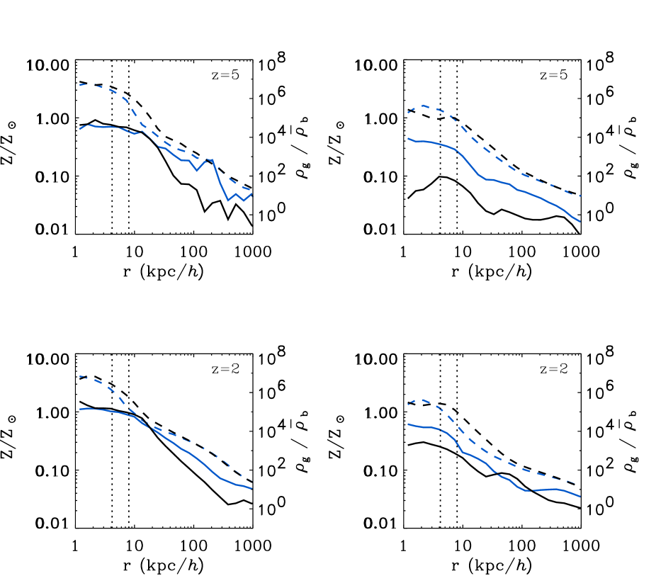
Figure 1.— Metallicity (left axis) and density profiles (right axis) shown with solid and dashed lines, respectively, of gas in halos of mass $M=2\times 10^{12}h^{-1}\hbox{$\rm\thinspace M_{\odot}$}$ (left panels) and $M=4\times 10^{10}h^{-1}\hbox{$\rm\thinspace M_{\odot}$}$ (right panels) at two different redshifts. The black lines show the results from the G5 simulation and the blue lines from the D5 run.

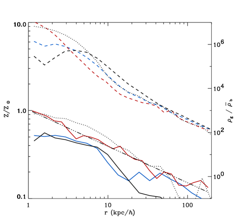
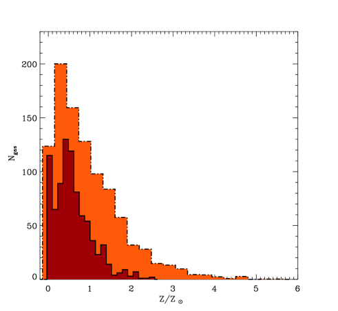
Figure 2.— Left panel: Metallicity (left axis) and density profiles (right axis) shown with solid and dashed lines, respectively, for halos of mass $M=2\times 10^{11}h^{-1}\hbox{$\rm\thinspace M_{\odot}$}$ (left panel) at redshift $z=3$. The black lines show the results from the G5 simulation and the blue lines from the D5 run. The red lines are for the Q5 simulation, and the dotted lines are for the P4 run, which is a model with weaker galactic winds. Right panel: Histogram for the metallicity of particles within 2  kpc in the two groups of mass $M=2\times 10^{11}h^{-1}\hbox{$\rm\thinspace M_{\odot}$}$ in the Q5 simulation.

Finally, an important feature of the simulations is that they include a phenomenological description of galactic winds. In this model, gas particles are stochastically driven out of the dense star-forming medium by assigning them extra momentum in random directions. It is assumed that the wind mass loss rate is proportional to the star formation rate, $\dot{M}_{W}=\eta\dot{M}_{*}$, and that its kinetic energy is comparable to the total available energy released by the supernovae associated with star formation, $\frac{1}{2}\dot{M}_{W}v_{W}^{2}=\chi\epsilon_{\rm SN}\dot{M}_{*}$. The simulations we use adopt a value of $\eta=2$ and $\chi=1$. This parameterization leads to an initial wind speed in the simulations equal to $484\,{\rm km\,s^{-1}}$. (For details, see e.g. Springel & Hernquist 2003a; Aguirre et al. 2001a,b.)

In order to resolve the full history of cosmic star formation, Springel & Hernquist (2003b) simulated a range of cosmological volumes with sizes ranging from $1\,h^{-1}$ Mpc to $100\,h^{-1}$ Mpc. For each box size, a series of simulations was performed where the mass resolution was increased systematically in steps of $1.5^{3}$, and the spatial resolution in steps of 1.5, allowing detailed convergence studies.

In this work, we show results mostly from the 100 $h^{-1}{\rm\thinspace Mpc}$ (runs G5 and G6), 33.75 $h^{-1}{\rm\thinspace Mpc}$ (D5 run), and $10h^{-1}{\rm\thinspace Mpc}$ (Q5 and P4 runs) boxes within the G-, D-, and Q/P-series, respectively (runs of the same boxsize are designated with the same letter, with an additional number specifying the resolution). We note that the G6 run is a new higher resolution version of the largest simulations described by Springel & Hernquist (2003b). The use of these multiple runs is important for studying the effects of numerical resolution. The Q/P-series can also be used to study the effects of wind strength. The fundamental properties of the simulations (particle number, mass resolution etc.) are summarized in Table 1. All length units that we quote throughout the paper are comoving, implying that at high $z$ the spatial resolution of the simulations in physical units is better than at low $z$.

In this work, it is important to analyze the larger boxes, as these allow us to study the rare large massive objects that host the quasars up to high redshifts and their evolution down to small redshifts. On the other hand, the smaller box of the Q-series allows us to assess the effects of numerical convergence and to study the physical properties of halos down to small distances from their centers.

3. Metallicity profiles versus halo mass

We identify groups of gas, stars and dark matter in the simulations by applying a conventional friends-of-friends algorithm to the dark matter, gas, and star particles. The specific details of the grouping method are described in Di Matteo et al. (2003). The center of each object is defined to be at the position of the gas particle with the highest density. We find indistinguishable results if we consider instead the gravitationally most bound particle. We then compute the radially averaged profiles of density and metallicity about these centers.

In Figure 1, we show the mean mass weighted metallicity profiles of gas (solid lines) as a function of radius for dark matter halos of mass $M=2\times 10^{12}h^{-1}\hbox{$\rm\thinspace M_{\odot}$}$ (left panels) and $M=4\times 10^{10}h^{-1}\hbox{$\rm\thinspace M_{\odot}$}$ (right panels) at $z=2$ and $z=5$ (top and bottom panels, respectively). Figure 1 also shows the mean density profiles normalized to the mean baryon density, $\bar{\rho_{b}}$. The metallicity and density profiles are calculated from both the G5 and D5 runs and are shown by the black and blue lines respectively. The vertical dotted lines represent the comoving gravitational softening lengths of the G5 and D5 runs, which are $8h^{-1}{\rm\thinspace kpc}$ and $4.17h^{-1}{\rm\thinspace kpc}$, respectively (see also Table 1). The comparison of metallicity and density profiles obtained from the G5 and D5 runs (black and blue lines respectively) is particularly instructive as we examine the effects of mass resolution on these physical quantities. Understanding the variation of these effects with radius will be important for our discussions in the rest of this paper.

For the large mass objects (left panel; $M=2\times 10^{12}h^{-1}\hbox{$\rm\thinspace M_{\odot}$}$), the metallicity profiles are characterized by a flat compact core extending to $r\sim 10\,h^{-1}{\rm\thinspace kpc}$, where $Z/Z_{\sun}\sim 1$. Outside this core, $Z/Z_{\sun}$ declines more significantly in the G5 run profiles than in the D5 run. Although in the inner regions the two simulations lead to similar values for the metallicity, we should be cautious in interpreting this, because the core component in the G5 run, and for some of the objects in the D5 run, appears around or within the simulations’ respective gravitational softening lengths. The presence of core components in the metallicity profiles may thus be due to lack of sufficient spatial resolution.

This last point seems to be reinforced by an examination of the density profiles. The mean gas density profiles measured in the G5 and D5 runs show fairly good agreement in the outer regions (for $\rho/\bar{\rho}_{b}\mathrel{\hbox to0.0pt{\lower 3.0pt\hbox{$\sim$}\hss}\raise 2.0pt\hbox{$<$}}10^{3-4}$) but the G5 profiles imply typically higher densities in the inner regions and again a flat density core within the resolution limits. Compared to the D5 results, those for the G5 run have enhanced densities in the core and a suppressed metallicity in the outer regions. This seems to indicate a lack of fully resolved star formation and efficient transport of metals by its associated feedback processes, at least with respect to the D5 simulation.

For the smaller mass objects ($M=4\times 10^{10}h^{-1}\hbox{$\rm\thinspace M_{\odot}$}$), the metallicity profiles in the G5 and D5 runs show larger discrepancies, as expected. In particular, the central metallicities measured in the G5 run are systematically lower than in the D5 simulation, where the metallicity profiles imply values of $Z/Z_{\sun}\sim 0.4-0.8$. The density profiles show overall agreement in the outer regions (at overdensities $\rho/\bar{\rho}_{b}\mathrel{\hbox to0.0pt{\lower 3.0pt\hbox{$\sim$}\hss}\raise 2.0pt\hbox{$<$}}10^{2}$) but the G5 profiles predict higher density values for distances less than few tens of  kpc, as a result of underresolved star formation and feedback in G5.

Although we expect the quasar hosts to reside in large mass halos, such as those plotted on the left in Figure 1 ($M\sim 10^{12}h^{-1}\hbox{$\rm\thinspace M_{\odot}$}$, see also §4.2), we would also like to understand the distribution of metals in the central regions of less massive groups, which the D5 and G5 runs are unable to resolve well. To do this, we turn to the Q5 simulation, which has much higher mass and force resolution (comoving gravitational softening length equal to $1.2\,h^{-1}{\rm\thinspace kpc}$). In Figure 2, we plot the metallicity (and density) distribution for objects in the Q5 simulation at $z=3$ (red lines). Because of the relatively small box ($10\,h^{-1}{\rm\thinspace Mpc}$ on a side) of the Q-series, the largest objects have masses of order $M\sim 10^{11}h^{-1}\hbox{$\rm\thinspace M_{\odot}$}$. We also show a direct comparison with the profiles of objects of the same mass measured in the D5 and G5 runs (blue and black lines, respectively). Finally, we include results from the P4 simulation (dotted line), which used the same size box as the Q-series but included a weaker model for winds, and a slightly lower resolution ($N=2\times 216^{3}$).

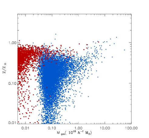
Figure 3.— Central values for the metallicities measured in the Q5 (red) and D5 (blue) simulations, as a function of the group gas mass in units of $10^{10}h^{-1}\hbox{$\rm\thinspace M_{\odot}$}$. The D5 run tends to underestimate the central metallicity values.

All the lines from the different simulations in Figure 2 represent averages over 2-3 objects with similar mass (and are therefore somewhat noisier than the profiles in Figure 1, which represented averages over a larger number of objects). The most significant feature to note in the comparison of the D5 and G5 results with the Q5 run is that while the metallicity profiles in the former simulations still show a core-like component in the central regions, the profile derived from the Q5 run continues to rise (the dash-dotted line represents a fit to the Q5 profile with a power law, in $\log$, of slope $\sim 0.4$) implying metallicity values in the center that are at least a factor $\sim 2$ higher than in the D5 and G5 runs.

In accord with Figure 1, the gas density profiles in Figure 2 show lower densities with improved resolution and fairly steep power law behavior of the density and metallicity profiles extending to the very central regions. Again this effect can be attributed to the improved numerical resolution in the Q5 simulation, which allows us to resolve higher gas densities and hence gas cooling, star formation and its associated feedback processes over a much larger range in scales. Finally the dotted lines in Figure 2 show the metallicity and density profiles obtained from the P4 run. This simulation was run with a weaker wind than the other simulations, with only half as much supernova energy deposited as kinetic energy of the wind. Comparing with the other profiles gives us some idea of the effects of the feedback by galactic winds. Within P4, we see an excess of metals and gas density in the center with respect to the other simulations. This is because the gas in the P4 simulation can cool and form stars more efficiently, without being blown away by winds as easily.

The right panel of Figure 2 shows a histogram of the metallicity values of the gas particles within $r\leq 2h^{-1}{\rm\thinspace kpc}$ for two groups in the Q5 simulation with $M\sim 10^{11}h^{-1}\hbox{$\rm\thinspace M_{\odot}$}$ (the profiles of which are shown in the left panel). This representation shows that the majority of the gas in these central regions has metallicity around solar (or below) but that there can be a relatively small fraction of gas with significantly super-solar metallicities in the inner regions.

Finally, in Figure 3 we show the values of the density weighted metallicity within the central $2h^{-1}{\rm\thinspace kpc}$ of all the objects in the Q5 run (red points) and those measured in the objects of the D5 run within the central $5h^{-1}{\rm\thinspace kpc}$ (blue points). The central metallicity values in the D5 run seem to be offset from those measured in Q5 and are typically lower by a factor $\sim 2$. Unfortunately, it is hard to assess whether this offset persists for the large mass objects in D5 which cannot be probed with Q5. However, by comparing the profiles in Figure 1 and Figure 2 we see no significant change in any of the general trends described above, and hence expect that the same offset in the central metallicity measurements is likely to persist up to the largest masses. In other words, because of the significant gradient in the metallicity profiles we have found in groups, we are not able to obtain quantitatively accurate measurements of the circumnuclear metallicity in the D5 or G5 simulations, because we are unable to resolve the relevant scales below the gravitational softening lengths of these simulations. Also note that the large dispersion in the central metallicity values in Figure 3, as measured in the D5 run at around $M_{\rm gas}\sim 0.1\times 10^{10}h^{-1}\hbox{$\rm\thinspace M_{\odot}$}$, is purely an artifact of insufficient resolution. This is directly demonstrated by comparing with the Q5 measurements.

In general, from the study of the metallicity profiles and the resolution studies discussed in this section, we can conclude that even within our model of quiescent star formation there appears to be a fairly strong metallicity gradient in massive galaxies. Regions of high density in the center of groups undergo strong star formation and enrichment. As a consequence, metallicities up to solar and super-solar values can easily be reached, at least in some fraction of the central gas. These results will be important for our discussions in the next section, and later when we compare our model with several recent measurements of circumnuclear gas in the high-$z$ QSOs.

4. Quasar metallicities

4.1. Quasar model

So far, we have examined the properties of friends-of-friends selected groups of gas and dark matter. In order to select quasar hosts from these and determine the quasar properties from the simulations (in which black holes have not been self-consistently included) we make use of the model developed by Di Matteo et al. (2003). Here we briefly summarize the main characteristics of this scheme and refer the reader to the above paper for details. The model starts from the hypothesis that black holes grow and shine by gas accretion, the supply of which is regulated by the interplay with star formation in spheroids. The black hole mass growth saturates in response to star formation and its associated feedback processes. This results in black holes masses that are related to the velocity dispersion of their host spheroids in a manner which is consistent with the observed $M-\sigma$ relation of Ferrarese & Merritt (2000) and Gebhardt et al. (2000). In this model, the QSO luminosity function evolves as a result of the declining amount of fuel available for accretion (and star formation), assuming a given (redshift independent) quasar lifetime and duty cycle. In Di Matteo et al. (2003) we also showed that within the context of this simple model the total black hole accretion rate (BHAR) density very closely tracks the star formation rate (SFR) density, as expected if black hole growth and fueling are fundamentally linked to the assembly of the spheroids and their star formation rate, respectively.

All galaxies are assumed to undergo active phases with a duty cycle given simply by $f_{Q}=t_{Q}/t_{H(z)}$, where $t_{Q}$ is the quasar lifetime and is the only free parameter of the model. In order to estimate the luminosity of each quasar, we simply assume that all the gas in the galaxy is in principle available for accretion on this timescale. The bolometric luminosity owing to accretion onto the central black hole at redshift $z$ is then given by

$$L=\eta\hbox{$\dot{M}$}(z)c^{2}\sim\eta\frac{\Delta M_{\rm gas}}{\Delta t}c^{2}\sim\eta fM_{\rm gas}(z)c^{2}/t_{Q},$$ (3)

where we have taken $\Delta M_{\rm gas}(z)\sim fM_{\rm gas}(z)$, assuming that the average mass accreted is a constant fraction $f$ of the total gas mass (see Di Matteo et al. 2003). We adopt the standard value for accretion radiative efficiency of $\eta=10\%$. With this model and $t_{Q}\sim 2-4\times 10^{7}{\rm\thinspace yr}$, we were able to reproduce the observed quasar luminosity function reasonably well, particularly for $z\mathrel{\hbox to0.0pt{\lower 3.0pt\hbox{$\sim$}\hss}\raise 2.0pt\hbox{$>$}}2$. A general feature of this model is that the black hole accretion rate history is found to closely follow the cosmic star formation rate density, therefore establishing a direct relation between black hole activity and star formation. A consequence of this is that at high redshifts we expect the evolution of black hole activity to be mostly driven by the gravitational growth of structure, as this is the case for the star formation rate density (Hernquist & Springel 2003) relatively independent of the details of the gas dynamics.

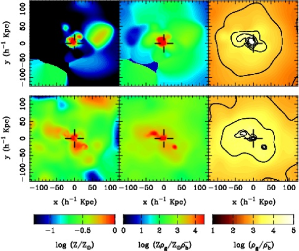
Figure 4.— Two quasar hosts in the G5 simulation, one at $z=5$ (top row) and one at $z=2$ (bottom row). For each host, we show from left to right the metallicity, the projected metal density (proportional to the mass of metals), and the gas density. The panels extend $250h^{-1}{\rm\thinspace kpc}$ in the $x$ and $y$ direction and $100h^{-1}{\rm\thinspace kpc}$ in the $z$-axis. and are centered on the quasars (positions shown by crosshairs). The quasars have magnitude $m_{B}=-26.3$ (top) and $m_{B}=-26.7$ (bottom) , and the corresponding masses of their host halos are $1.8\times 10^{12}h^{-1}\hbox{$\rm\thinspace M_{\odot}$}$ and $3.1\times 10^{12}h^{-1}\hbox{$\rm\thinspace M_{\odot}$}$, respectively.

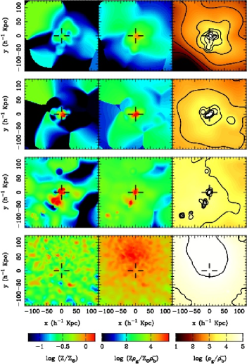
Figure 5.— Time evolution of a gas element initially identified in a quasar host at $z=6.5$. We show metallicity (left panels), projected metal density (center panels), and projected gas density (right panels), for slices of $100h^{-1}{\rm\thinspace kpc}$ width in the $z$-direction and and 250 $h^{-1}{\rm\thinspace kpc}$ in $x$ and $y$ (same as Fig. 4). The top row of panels shows the situation at $z=6.5$, centered on the quasar position. At this time the quasar has absolute magnitude $m_{B}=-26.2$ and resides in a halo of mass $1.1\times 10^{12}\hbox{$\rm\thinspace M_{\odot}$}$. In the succeeding three rows, each panel is centered on the position of the particle which was the most bound at $z=6.5$ (closest to the quasar), but at the later redshifts of $z=4$, $z=2$, and $z=0$.

4.2. The quasar hosts

Table 2 Quasar host properties.

Redshift	$M_{\rm DM}$	$M_{\rm BH}$	$SFR$
	$10^{12}h^{-1}\hbox{$\rm\thinspace M_{\odot}$}$	$10^{9}h^{-1}\hbox{$\rm\thinspace M_{\odot}$}$	$\hbox{$\rm\thinspace M_{\odot}$}{\rm\thinspace yr}^{-1}\,$
2	$3$	$1.3$	$38$
5	$1.8$	$0.9$	$600$
6.5	$1$	$0.8$	$270$

Visualizing the morphology of the metal-rich gas in and around quasar hosts can tell us directly how the metal enrichment occurs in these high density loci and how uniformly the metals are distributed in response to star formation and its associated feedback. In Figure 4, we show a plot of the hosts of two typical bright quasars (with $B$-band magnitude $m_{\rm b}<-26$), which were picked randomly from the $z=5$ and the $z=2$ outputs of the G5 simulation. In Table 2, we summarize some of the main properties of these hosts, such as their dark matter, stellar and black hole masses together with their central star formation rates. In both cases, the metallicity close to the center (indicated by the cross on the figure) is around solar, and the mass of their host halos is similar and of the order of a few $10^{12}h^{-1}\hbox{$\rm\thinspace M_{\odot}$}$. The $z=5$ quasar rests in a more concentrated island of metal rich gas than the $z=2$ case, where the edges of the central enhancement are more diffuse. It is evident, therefore, that although the mean metallicity of the ISM is lower at $z=5$, the central regions do not show significant evolution. We find that in the central regions, star formation, and consequently metal enrichment proceeds rather quickly because of the high densities entailing short star formation timescales (Eq. 2).

This plot also shows that star formation occurs in islands of high gas density that lie nearby in the $z=2$ case, so that the high metallicity of the gas 50 to 100 $h^{-1}{\rm\thinspace kpc}$ away from the quasar has likely been generated in situ rather than being blown there by winds. We note that the star formation rate in the object at $z=5$ is about a factor 15 higher than in the object at $z=2$, suggesting that the massive hosts of high redshift quasars are likely to be associated with more significant star formation activity.

As well as examining at the central region of different bright quasar hosts active at different redshifts, we can also look at the history of gas that was once at the center of an early quasar. In this way, we can see how the large scale movements of hosts through the evolving density field impact their metallicity and study the relationship between the quasar phase and the first major star formation event. In Figure 5, we follow the position of what was initially the most tightly bound particle in one of the earliest bright quasars to be active in the G5 simulation, at $z=6.5$. We can see that at $z=6.5$, the metallicity near the center of the host is well below solar, although the mass of the halo is relatively high, of order $\sim 10^{12}h^{-1}\hbox{$\rm\thinspace M_{\odot}$}$. Because in our model the quasar phase is dependent only on the amount of gas in the halo, it can, at these early times, be coeval with the first major event of star formation in the galaxy. We note that the star formation rate in the galaxy measured in the simulation corresponds to $\sim 200\hbox{$\hbox{$\rm\thinspace M_{\odot}$}{\rm\thinspace yr}^{-1}\,$}$ (see Table 2). The metallicity builds up rapidly to values of around solar in the central region by the $z=4$ timeslice (and according to Fig. 4 probably by $z=5$) although outside $\sim 20h^{-1}{\rm\thinspace kpc}$ not much has changed. By $z=2$, the particle has moved into a large scale overdensity, presumably a forming cluster, and is beginning to be surrounded by metal-rich gas. At $z=0$, the particle is approximately $75h^{-1}{\rm\thinspace kpc}$ from the center of a cluster, which can be clearly seen in the distribution of metal density. The cluster has no obvious metallicity gradient (at least in the central portion that can be seen), with no remnant of the tight knot of high metallicity which was seen in the earlier redshift panels. The particle which was once close to the center of a quasar host at $z=6.5$ is now surrounded by gas with $Z\sim 0.3$ solar, typical of the intracluster medium (ICM) observed today.

Although Figure 5 shows only one particular example of the evolution of the environment of a high redshift quasar, other quasars, which are bright at these redshifts will have similar histories. At $z\sim 6-7$ the gas in these high overdensity regions, where quasars are located, necessarily evolves to form the central regions of clusters at low redshifts.

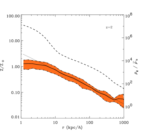
Figure 6.— Mean metallicity (left axis) in units of solar metallicity, and density profiles in units of the mean baryon density (right axis), shown with solid and dashed lines, respectively, for the bright quasars ($m_{b}<-26$) at $z=2$ (D5 run). The red area represents the standard deviation from the mean metallicity profile. Note the similarity between these profiles and those for halos of mass $M=2\times 10^{12}h^{-1}\hbox{$\rm\thinspace M_{\odot}$}$ shown in Figure 1. The dotted line shows an extrapolation into the central region obtained by fitting a power law to the outer regions (see text).

5. Mean quasar metallicity evolution

5.1. The circumnuclear metallicity

In Figure 6, we show the mean quasar metallicity profile and the mean normalized density profile at $z=2$ for the bright $m_{b}<-26$ quasars. The orange area shows the standard deviation about the mean metallicity values, and the dotted line gives a power law fitted to the region outside the core of the profile (outside $r\sim 10h^{-1}{\rm\thinspace kpc}$). Because we have seen that quasars reside in large mass halos (see also §4) we can only study their properties directly in the larger simulation boxes of the D5 and G5 simulations. However, according to the analysis of the numerical convergence in the metallicity profiles in §3, we expect that the true metallicity profiles should exhibit a power law behavior which continues further into the central regions.

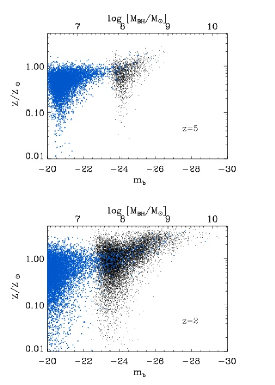
Figure 7.— Metallicity versus B-magnitude ($m_{b}$) for all objects in the D5 simulation (blue points) and G5 simulation (black) at redshift $z=2$ and $z=5$. The comparison between the two different runs shows that there is very little dependence of metallicity on $m_{\rm b}$. The large scatter seen at low $m_{b}$ is an artifact owing to the lack of sufficient resolution close to the mass resolution limit of the respective simulation.

It is important to determine the central metallicities from the simulations because the observed quasar metallicities come exclusively from the spectroscopic studies of the broad line region and hence probe the metal enrichment of gas that is in the inner, high density regions of the galaxy. Here, we would like to compare the quasar metallicities obtained from our model to those observed. Given the relatively strong metallicity gradient that we have found in the previous sections, and in Figure 6, it is necessary to estimate the metallicity close to the center.

We use the behavior seen in the higher resolution Q5 run to apply a correction to the metallicities of the quasar hosts in the D5 and G5 simulations. The power law behavior seen in the central parts of the Q5 galaxies is assumed to apply to the central regions of the D5 and G5 objects as well. As explained above, we cannot explicitly test the validity of this well-motivated correction for the most massive galaxies which make up the hosts of high redshift quasars at presently observed magnitude limits. This would require yet more demanding simulations that combine box sizes comparable to that of G5 with a mass resolution as good as that of Q5. However, we note that at present, even without our correction, the measured simulation metallicities represent a robust lower limit, which is above solar, even at high redshifts. The metallicities of QSOs fainter than have yet been observed can be predicted without extrapolation and we shall do this as well.

For each quasar, we calculate a value for the circumnuclear metallicities by integrating the metallicity profile mass weighted out to the radius $R_{6}$ corresponding to an overdensity of $\rho/\bar{\rho}_{b}=10^{6}$ (which typically corresponds to a few  kpc). The metallicities are then given by

$$Z=\frac{\int_{0}^{R_{6}}\rho(r)Z(r)\,{\rm d}r}{\int_{0}^{R_{6}}\rho(r)\,{\rm d}r}.$$ (4)

Because we compute mass weighted metallicity and the slope of the density profile is relatively shallow in the central regions, our results are fairly insensitive to the density threshold.

In Figure 7, we plot the circumnuclear metallicities obtain in this way as a function of the quasar $m_{b}$ magnitude at $z=5$ and $z=2$, both for the G5 simulation (black points) and the D5 simulation (blue points). The plot shows a moderate trend of increasing metallicity with decreasing quasar magnitude (although this trend breaks down close to the mass resolution of the respective simulation, where the scatter in the points is seen to increase significantly). This trend is broadly similar to that found by Dietrich et al. (2003b) between metallicity and continuum luminosity ($L_{\alpha}$) in a sample of high redshift quasars. It is also consistent with the luminosity-metallicity relation for quasars (Hamann & Ferland 1993; 1999, Shemmer & Netzer 2003). Since we assume universal values for the quasar lifetime and accretion efficiency, there is a unique black hole mass corresponding to a given quasar luminosity. The top axis in Figure 7 shows this corresponding black hole mass for the objects, and hence gives the relation between $Z/Z_{\sun}$ and $M_{\rm BH}$ inferred from the simulations and the model.

5.2. Comparison with observations

In Figure 8, we compare observations of quasar metallicities up to $z\sim 8$ with the mean quasar metallicity evolution obtained from the simulations for four possible values of the quasar lifetime, $t_{Q}=4,\;2,\;1,\;{\rm and}\;0.5\times 10^{7}{\rm\thinspace yr}$ (solid, dashed, dash-dotted, dotted lines, respectively). The lines show the predictions for the mean circumnuclear metallicity for the bright quasars, $m_{b}<-26$, which can be directly compared with the observations. The black lines are the results from the G5 simulation, the pink lines from the G6 and the blue lines are from the D5 run.

The observational data from Dietrich et al. (2003a,b) and Freudling et al. (2003) represent individual quasar metallicities (solid black and grey points, respectively). The open squares show the mean metallicity and standard deviation of a sample of quasars from Iwamuro et al. (2002), the open circles are the mean metallicities from a sample of quasars of comparable luminosities studied by Dietrich et al. (2003c) and the diamonds from a sample of 22 quasars studied by Maiolino et al. (2003). In all these works, the metallicity of the gas associated with the quasars is estimated from a study of the broad emission line region (BELR) in the ultraviolet spectral range using photoionization models (see, e.g., the review by Hamann & Ferland 1999). The BELR spans a range of distances from a fraction of a pc to a few pc from the central object, so that it probes the physical conditions of gas in the circumnuclear region of a quasar.

The solid points in Figure 8 represent the chemical abundances calculated by Dietrich et al. (2003a,b) from emission line ratios of several different elements. In particular, nitrogen lines were related with lines of helium, oxygen and carbon, and the results from photoionization calculations of Hamann et al. (2002) were employed. The open squares, open circles, open diamonds and grey points represent measurements of the MgII/FeII ratio from Iwamuro et al. (2002), Dietrich et al. (2003c), Mailino et al. (2003) and Freudling et al. (2003), respectively, which have been converted into a metallicity using the flux ratio of 2.75 expected for solar metallicities (derived using photoionization models; see Freudling et al. 2003; Wills, Netzer & Wills 1985). As these last three sets of data points have been obtained by converting values of MgII/FeII directly into a metallicity they should be regarded as a far less reliable indicator of the overall metallicity than the Dietrich et al. (2003a,b) data.

The lines in the bottom panel of Figure 8 show the standard deviation, divided by the mean gas metallicity, of the quasar population in the simulations. For comparison, we have also computed the standard deviation of the observed quasar metallicities in three redshift bins (solid yellow points). For this calculation, we subtracted the measurement errors in quadrature in order to give us an estimate of the intrinsic scatter in metallicity between quasars. The resulting values are plotted as symbols in Figure 8, with Poisson error bars. Realistically, these values should probably be taken as upper limits on the standard deviations because of the uncertainties in the photoionization modeling used to convert line ratios to metallicities. However, their magnitude is comparable to the standard deviations from the simulations.

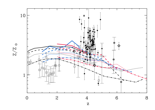
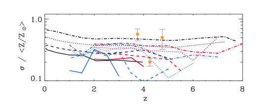
Figure 8.— Evolution of the mean gas metallicities (top panel) and standard deviations (bottom panel) of QSOs with $m_{b}<-26$ as a function of redshift. The results from the D5 (blue lines), G5 (black lines) and G6 simulation runs (pink lines) are shown with solid, dashed, dotted, dash-dotted lines for quasar lifetimes $t_{\rm Q}=4,\;2,\;1,\;0.5\times 10^{7}\,{\rm yr}$, respectively. The black solid dots show the measurements of individual quasar metallicities by Dietrich et al. (2003a,b). The solid grey points show the measurement of the flux ratio FeII/MgII of 3 SDSS high redshift quasars (Freudling et al. 2003), translated into $Z/Z_{\sun}$ by using the factor 2.75 expected for solar abundances (Wills, Netzer & Wills 1985). The open squares show the median and standard deviation (the error bar) from a large sample of quasars for which the FeII/MgII flux ratio was measured (Iwamuro et al. 2002), the open circles show the same average ratio of FeII/MgII measured by Dietrich et al. (2003c) from a sample of comparable luminosity and the open diamonds from a sample of 22 quasar measured by Maiolino et al.(2003). The same rescaling factor as above was used to obtain the corresponding metallicities. Metallicities shown from these last three sets of observations are more uncertain than the Dietrich et al. (2003a,b) values. In the bottom panel, the yellow solid circles show the standard deviation of the quasar metallicities in the Dietrich et al. (2002) sample in three redshift bins. The error bars represent Poisson errors.

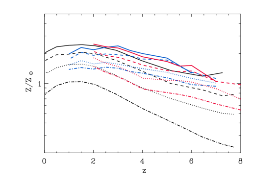
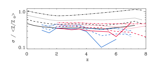
Figure 9.— Same as Figure 8, but including QSOs of lower luminosity, down to a cutoff of $m_{b}<-24.5$. No data is shown since a direct comparison with observations is not yet possible.

The mean metallicity of the gas in the circumnuclear region (as defined in Eq. 4) measured in the simulations reaches values of $Z\sim 1-3\,Z_{\sun}$, with the highest supersolar values corresponding to the longest quasar lifetime, $t_{Q}\sim 4\times 10^{7}{\rm\thinspace yr}$. This trend with $t_{Q}$ is expected because by assuming a longer quasar lifetime we select very rare high-density peaks to be the hosts of quasars, whereas a lower timescale implies that quasars that turn on are found in less biased host galaxies. Note also that the longer timescales, in our model, are also those that best reproduce the quasar luminosity function, particularly at $z\mathrel{\hbox to0.0pt{\lower 3.0pt\hbox{$\sim$}\hss}\raise 2.0pt\hbox{$>$}}3$ (Di Matteo et al. 2003). The corresponding mean gas metallicities of these massive hosts (see also Fig. 4) are comparable to the range inferred from the observations of the BELRs (Figure 8). We emphasize that the supersolar metallicities in the simulations are associated with the relatively small fraction of the highest density gas that resides in the innermost regions of the galaxy (see also Figs. 2 and 6). The mean metallicity of the gas in galaxies as a whole is much lower and reaches at best a tenth to a few tenths of the solar value (see Fig. 6). It is likely, therefore, that the supersolar chemical abundances measured in quasars are representative only of the highest density gas in the centers of galaxies which has undergone star formation on a short dynamical timescale.

We also note that the mean quasar metallicity shows virtually no evidence of an evolutionary trend out to redshift $z\sim 5$ (see in particular the results for the D5 run), which is consistent with all the current observations (e.g. Dietrich et al. 2003a,b). We predict, however, a slow decline of the mean metallicity above this redshift, even though solar-like values are still attained in the high-density gas up to redshift $z\mathrel{\hbox to0.0pt{\lower 3.0pt\hbox{$\sim$}\hss}\raise 2.0pt\hbox{$<$}}7$.

The differences at $z\mathrel{\hbox to0.0pt{\lower 3.0pt\hbox{$\sim$}\hss}\raise 2.0pt\hbox{$>$}}3$ between the results from the G5 and D5 runs are due to numerical resolution (as also shown in Figure 3 and Figure 7). The higher resolution runs (like the D5 or Q5) are able to resolve smaller halos, which are present abundantly at high redshift, better than the low resolution runs. This means, for example, that the D5 run has more star formation, and consequently more metal production at high redshift than the G5 simulation. On the other hand, because of the relatively small box size of the D5 run, the largest objects that contribute to the magnitude limit of $m_{b}<-26$ are very rare at high-$z$. Making use of the G6 simulation, which has the large box and higher resolution than the G5 (intermediate between the D5 and G5; see Table 1), we find that for some objects, convergence is in fact achieved. This is the case for the longest timescales, which restrict quasar hosts to the most massive objects only. In this case, the G6 results are consistent with those from the G5 run, as we would expect given that star formation in these most massive halos has been resolved. The increase in metallicities from redshifts $z\sim 8$ to $z\sim 5$ is therefore likely to be real in these objects. For shorter timescales, however, the hosts have typically smaller masses on average, and convergence is not quite attained (as shown by the comparison between the G6 and D5 results). Even so, the evolution of the metallicity for these timescales is expected to be flatter than for the longer timescales.

It is difficult, therefore, to predict the evolution of the metallicity beyond redshift $z\sim 5$ in Figure 8 for all quasar timescales reliably. For this reason, and in order to probe the quasar and halo mass function up to higher redshifts, we include quasars with lower luminosity down to $m_{b}<-24.5$ in the results shown in Figure 9 (which otherwise has the same format as Figure  8). Because of the inclusion of a larger number of smaller mass halos in this magnitude cut, the difference between the D5 and G5 runs is increased whereas the G6 and the D5 results do show convergence for the larger timescales. The general trend of no or very mild evolution in the gas metallicity is consistent with that in Figure 8. In addition, we note that shorter quasar lifetimes seem to imply slightly stronger evolution beyond $z\sim 5$ than the longer lifetimes. Note that the dispersion about the mean is also larger than in Figure 8. This is expected given the metallicity-luminosity relation we have found in Figure 7, because we have now considered a larger range of quasar magnitudes.

By including objects with lower quasar luminosities we are actually considering those which are less massive and hence more abundant at high redshifts. Because of the steep cut-off in the halo mass function at high redshifts and the association of bright quasars ($m_{b}<-26$) with dark matter masses of the order of $M\sim 10^{12}h^{-1}\hbox{$\rm\thinspace M_{\odot}$}$, we simply cannot expect to find these bright objects beyond $z\sim 8$. This implies that in order for observations to resolve the bulk of the black hole activity beyond these redshifts, instrument sensitivities need to account for the characteristically lower quasar luminosities in this regime. If this can be achieved, the measurement of quasar metallicities provides a potentially useful new probe for the quasar lifetime and therefore a test of the characteristic black hole mass function at high redshifts.

6. Discussion

We have used cosmological hydrodynamical simulations coupled with a prescription for black hole activity in galaxies to study the evolution of the metal enrichment in quasar host galaxies and explore the relation between star/spheroid formation and black hole growth/activity. In the black hole accretion model developed in Di Matteo et al. (2003), the black hole fueling rate is regulated by its interplay with star formation and associated feedback processes in the gas. This establishes a link between star formation and the quasar phase in host galaxies, which in turn can broadly reproduce the observed slope of the relation between black hole mass and stellar velocity dispersion, as well as the properties of the X-ray and optical QSO luminosity functions. In this model, the black hole accretion rate density is found to closely track the star formation rate density of the simulations, as expected when black hole growth and fueling are fundamentally linked to the assembly of their host spheroids.

Using simulations with different resolution, we have measured the distribution of the gas metallicity and density in quasar host galaxies (and non-hosts) from $z=8$ to $z=0$. We typically find a strong radial gradient in the metallicity of the gas in halos, with the central densest regions of galaxies reaching up to a few times the solar metallicity (in the most massive objects) while the gas in the outer regions has a metallicity which is at most around a few tenths of solar. The more pronounced metal enrichment in the central regions is a natural consequence of the star formation model in the simulations which depends on the local gas density and hence occurs on the shortest timescales in the densest gas ($t_{*}\propto\rho^{-1/2}$).

We compared the results from the simulations with the observed values of gas metallicity estimated from the broad emission line region of bright quasars (e.g. Dietrich et al. 2002, 2003a,b). The simulations suggest that the super-solar metallicities of quasars deduced from these studies are representative of the highest density gas that resides in the innermost regions of galaxies. In this picture, the very high metallicities probed by the BELR are found only in a very small fraction of the gas, within the nuclear regions that undergoes the fastest modes of star formation and chemical enrichment. In other words, the self-regulated, quiescent mode of star formation implemented in the simulations can account well for the mildly super-solar metallicity of the gas seen around bright quasars.

In agreement with observations, the simulations predict little or no evolution of the mean quasar metallicity in the measured redshift range of $3.5<z<5$ (Dietrich et al. 2003a,b). The mean metallicity of quasars with $m_{b}<-26$ is predicted to be $Z\sim 2-3\,Z_{\sun}$ over the redshift range $0<z<5$, with a drop by a factor of 2-3 at earlier times (for $5<z<8$). The high, solar/super-solar-like metallicities at high redshifts are achieved quickly in rare and isolated islands of high-density gas residing in the first halos that form. They thus indicate the presence of massive star formation already at $z\sim 6-7$ (see Figs. 4 and 5). The scatter between quasars is likely to give us an idea of the scatter between host formation times, or between the times of recent major star formation episodes. Note that the mean gas metallicity of the quasar hosts is around $~{}0.1-0.5Z_{\sun}$, typical of massive galaxies throughout the redshift range.

We also find a mild dependence of metallicity on quasar luminosity (and hence black hole mass; Fig. 7) which appears to be consistent with observed trends (e.g. Hamann & Ferland 1999; Dietrich et al. 2003b; but see also Shemmer & Netzer 2002).

We note that within the ‘standard’ mode of star formation modeled by the simulations, the gas metallicity rarely exceeds $Z\sim 4-5\,Z_{\sun}$ whereas some of the most extreme observed values are reported to be as large as $Z\sim 10\,Z_{\sun}$. As we have seen from our convergence tests, the lack of fully resolved star formation at these high redshifts may still cause us to miss some metal enrichment. However, the observed values also bear significant uncertainties owing to the complex modeling that goes into the measurement of metal abundances from BELR observations. If such high observed metallicities are indeed present, their proper explanation may require higher yields and hence a top-heavier IMF compared to that in our simulations (which assume a solar yield). The net yield is related to the IMF $\phi(m)$ by

$$y=\sum_{k}\frac{\int_{m_{l}}^{m_{u}}m\,p_{k}(m)\phi(m)\,{\rm d}m}{1-\int_{m_{l}}^{m_{u}}[m-w_{k}(m)]\phi(m)\,{\rm d}m},$$ (5)

where $p_{k}(m)$ is the stellar yield of the $k$-th element, and $w_{k}(m)$ is the remnant mass of initial mass $m$. Using $w_{k}$ and $p_{k}$ values tabulated by Portinari, Chiosi & Bressan (1998) and Marigo (2001) for the mass ranges $6\hbox{$\rm\thinspace M_{\odot}$}<m<120\hbox{$\rm\thinspace M_{\odot}$}$ and $0.8\hbox{$\rm\thinspace M_{\odot}$}<m<6\hbox{$\rm\thinspace M_{\odot}$}$, respectively, and assuming $\phi(m)={\rm d}N/{\rm d}m\propto m^{-(1+a)}$, we find that an IMF-slope of $a\sim 1.1$ is required to reach a yield approximately twice the solar value, which is flatter than the Salpeter-IMF with $a=1.35$. For such a shallower, yet plausible IMF we would then expect (for a simple closed-box model) that metallicities become larger by about the same factor of two. The presence of extreme objects like these quasar hosts with highly super-solar metallicities would then (if confirmed) imply that such different forms of IMF exist, at least in the central high density regions of galaxies. It will be interesting to investigate, with larger observational samples, whether such extreme objects can only be found at high redshift, and whether there is any evolution of this extreme population and hence of the typical IMF of massive hosts.

A further constraint on the IMF in the models can be provided by considering the ionizing background radiation produced by stars in high redshift galaxies. The observed Lyman-$\alpha$ optical depth in high redshift quasars constrains the intensity of this radiation. In Sokasian et al. (2003a,b) the star formation rates from the simulations were used to predict the intensity of the background radiation. Good agreement was found with Ly-$\alpha$ observations, assuming an escape fraction of $20\%$ for the ionizing photons. Changing the IMF to make it flatter would increase the production rate of ionizing photons, so that a lower escape fraction would be necessary to match observations. With prior information on the escape fraction, a measurement of the Ly-$\alpha$ optical depth could yield a more direct constraint on the IMF.

We have shown that the highest values for the mean metallicity, and hence those which best agree with observations, are obtained for assumed quasar lifetimes in the range $4\times 10^{7}\mathrel{\hbox to0.0pt{\lower 3.0pt\hbox{$\sim$}\hss}\raise 2.0pt\hbox{$>$}}t_{Q}>10^{7}{\rm\thinspace yr}$. This is consistent with bright quasars residing in very massive host galaxies. Shorter quasar lifetimes place quasars also in less massive hosts where we find that the gas can only achieve metallicity up to solar like values. This agrees with the quasar luminosity (and black hole mass)-metallicity relation that we have shown in Figure 7. We note, coincidentally, that this range of quasar lifetimes is consistent with constraints obtained from studies of the reionization of HeII (e.g. Sokasian, Abel & Hernquist 2002, 2003).

Taking into consideration the metallicity inferred from the $\alpha$ elements (the ratio of MgII/FeII), which span a larger range of redshift, we see that there is an evolution towards lower metallicities for quasars at $z\mathrel{\hbox to0.0pt{\lower 3.0pt\hbox{$\sim$}\hss}\raise 2.0pt\hbox{$<$}}2$. This may suggest that below $z\sim 2$ nuclear activity takes place in more common hosts, or equivalently, that the quasar lifetimes are shorter than in the high redshift quasars (but note that these measurements have more significant uncertainties when used to infer global metallicities than those obtained from N, O, and C, and maybe also include objects spanning a larger range of luminosities).

Using the simulations, we can directly look at the predicted properties of quasar host galaxies at high redshifts. In our model, bright rare quasars at $z\mathrel{\hbox to0.0pt{\lower 3.0pt\hbox{$\sim$}\hss}\raise 2.0pt\hbox{$>$}}5$ reside typically in massive dark matter potentials, with $M_{\rm DM}\sim$ a few $10^{12}h^{-1}\hbox{$\rm\thinspace M_{\odot}$}$, characterized by high star formation rates of the order of $10-100\hbox{$\hbox{$\rm\thinspace M_{\odot}$}{\rm\thinspace yr}^{-1}\,$}$. Therefore, quasars reside in the rare, most massive halos which are already forming stars vigorously at these times. Most of the black hole growth occurrs simultaneously with the processes that dump matter into the central regions of galaxies and induce substantial star formation. In particular, under the assumption that the black hole mass is proportional to the mass of gas, we find typical black hole masses for these objects of order $M_{\rm BH}\sim 10^{9}\hbox{$\rm\thinspace M_{\odot}$}$. We find that the quasar phase at high redshift follows or is roughly co-eval with the major star formation event in these massive objects (see Figs. 4 and 5). These results are consistent with sub-mm and IR observations of high redshift quasars which imply large luminosities in these bands and hence gas rich, strongly star forming hosts (Omont et al. 2001; Archibald et al 2001; Pridley et al. 2003).

The results we have discussed here further strengthen the evidence for a strong relation between galaxy formation, star formation and black hole activity, and hence underline the importance of quasar studies for understanding high-redshift star formation and early galaxy evolution. Using the simulations and the measured metal abundances, we have shown that it is possible to construct self-consistent models for the locations where massive galaxies are being assembled, vigorously forming stars and building central black holes. As more precise measurements of quasar metallicities become available, it may therefore become possible to use these models to much better constrain the parameters which govern the stellar mass function in the redshift range where the large quasar hosts were forming. It should be within the capabilities of forthcoming millimeter array telescopes (like ALMA) and the James Webb space Telescope (JWST) to observe quasars in this fashion up to redshift $z\sim 8$ and beyond.

REFERENCES

Aguirre, A., Hernquist, L., Schaye, J., Weinberg, D., Katz, N., Gardner, J., 2001a, ApJ, 560, 599

Aguirre, A., Hernquist, L., Schaye, J., Katz, N., Weinberg, D., Gardner, J., 2001b, ApJ, 561, 521

Archibald, E. N., Dunlop, J. S., Hughes, D. H., Rawlings, S., Eales, S. A., & Ivison, R. J. 2001, MNRAS, 323, 417

Carilli, C. L., Bertoldi, F., Menten, K. M., Rupen, M. P., Kreysa, E., Fan, X., Strauss, M. A., Schneider, D. P., Bertarini, A., Yun, M. S., Zylka, R., 2000, ApJ, 533, L13

Carilli, C. L., Kohno, K., Kawabe, R., Ohta, K., Henkel, C., Menten, K. M., Yun, M. S., Petric, A., Tutui, Y., 2002, ApJ, 569, 605.

Ciotti L., van Albada T.S., 2001, ApJ, 552, L13

Cox, P., Omont, A., Djorgovski, S. G., Bertoldi, F., Pety, J., Carilli, C. L., Isaak, K. G., Beelen, A., McMahon, R. G., Castro, S., 2002, A & A, 387, 406

Croft R. A. C., Di Matteo T., Davé R., Hernquist L., Katz N., Fardal M. A., Weinberg D.H., 2001, ApJ, 557, 67

Davé, R., Hernquist, L., Katz, N., Weinberg, D.H., 1999, ApJ, 511, 521

Dietrich, M., Appenzeller, I., Wagner, S. J., G ssler, W., Hafner, R., Hess, H.-J., Hummel, W., Muschielok, B., Nicklas, H., Rupprecht, G., Seifert, W., Stahl, O., Szeifert, T., Tarantik, K., 1999, A&A, 352, L1

Dietrich M., Appenzeller I., Vestergaard M., Wagner S.J., 2002, ApJ, 564, 581

Dietrich M., Appenzeller I., Hamann F, Heidt J., Jager K., Vestergaard M. & Wagner S.J., 2003a, A&A, 398, 891

Dietrich M., Hamann F., Shields J.C., Costantin A., Heidt J., Jager K., Vestergaard M., Wagner S.J., 2003b, ApJ, 589, 722

Dietrich M., Hamann F., Appenzeller I., Vestergaard M., 2003c, ApJ, 596, in press

Di Matteo T., Croft R.A.C., Springel V., Hernquist L., 2003, ApJ, 593, 56

Efstathiou, G & Rees, M. J., 1988, MNRAS, 230, 5

Ferrarese L. & Merritt D., 2000, ApJ, 539, L9

Freudling W., Corbin M.R., Korista K.T., 2003, ApJ, in press [astro-ph/0303424]

Gebhardt K. et al., 2000, ApJ, 539, L13

Granato G.L., De Zotti G., Silva L., Bressan A., Danese L., 2003, submitted [astro-ph/0307202]

Haiman Z., Ciotti L., Ostriker J.P., 2003, ApJ, submitted [astro-ph/0304129]

Hamann, F., Ferland, G., 1993, ApJ, 418, 11

Hamann, F., Ferland, G., 1999, ARA&A, 37, 487

Hamann, F., Korista, K. T., Ferland, G. J., Warner, C., Baldwin, J., 2002, ApJ 564, 592

Hernquist L., 1993, ApJ, 404, 717

Hernquist L., Springel V., 2003, MNRAS, 341, 125

Iwamuro, F., Motohara K., Maihara, T., Kimura M., Yoshi Y., Doi M., 2002, ApJ, 565, 63

Katz, N., Weinberg, D.H., Hernquist, L., 1996, ApJS, 105, 19

Kauffmann G., Haehnelt M., 2000, MNRAS, 311, 576

Kennicutt, R.C.Jr., 1998, ARA&A, 36, 189

Kogut, A. et al., 2003, ApJ, submitted [astro-ph/0302213]

Kormendy J., Gebhardt K., 2001, In Wheeler J.C. Martel H. eds, AIP Conf. Proc. Vol. 586, 20th Texas Symposium On Relativistic Astrophysics. Am. Inst. Phys., New York, p.363

Magorrian et al., 1998, AJ, 104, 372

Maiolino R., Juarez Y., Nagar N.M., Oliva E., 2003, ApJ, in press, [astro-ph/0307264]

Marigo P., 2001, A&A, 370, 194

Merritt D., Ferrarese, L., 2001, MNRAS, 320, L30

Monaco, P., Salucci P., & Danese L., 2000, MNRAS, 311, 279

Omont, A., Cox, P., Bertoldi, F., McMahon, R. G., Carilli, C., & Isaak, K. G. 2001, A&A, 374, 371

Portinari L., Chiosi C., Bressan A., 1998, A&A 334, 505

Pridley R.S., Isaak K.G., McMahon R.G., Robson E.I., Pearson C.P., 2003, MNRAS, submitted [astro-ph/0308132]

Shemmer O. & Netzer H., 2002, ApJ, 567, L19

Sokasian, A., Abel, T., & Hernquist, L. 2002, MNRAS, 332, 601

Sokasian, A., Abel, T., & Hernquist, L. 2003, MNRAS, 340, 473

Sokasian, A., Abel, T., Hernquist, L., & Springel, V. 2003a, MNRAS, 344, 607

Sokasian, A., Abel, T., Hernquist, L., & Springel, V. 2003b, MNRAS, submitted [astro-ph/0307451]

Springel V., Hernquist L., 2002, MNRAS, 333, 649

Springel V., Hernquist L., 2003a, MNRAS, 339, 289

Springel V., Hernquist L., 2003b, MNRAS, 339, 312

Springel V., Yoshida, N., White, S.D.M., 2001, NewA, 6, 79

Tremaine S. et al. 2002, ApJ, 574, 740

Wills B., Netzer, H., Wills, D., 1985, ApJ, 288, 94

Wyithe J.S., Loeb A., 2002, ApJ, 581, 886

Yoshida, N., Sokasian, A., Hernquist, L., & Springel, V., 2003a, ApJ, 591, L1

Yoshida, N., Sokasian, A., Hernquist, L., & Springel, V., 2003b, ApJ, in press [astro-ph/0305517]