Large-scale structure and matter
in the universe

Abstract

Cosmology – Galaxies: clustering This paper summarizes the physical mechanisms that encode the type and quantity of cosmological matter in the properties of large-scale structure, and reviews the application of such tests to current datasets. The key lengths of the horizon size at matter-radiation equality and at last scattering determine the total matter density and its ratio to the relativistic density; acoustic oscillations can diagnose whether the matter is collisionless, and small-scale structure or its absence can limit the mass of any dark-matter relic particle. The most stringent constraints come from combining data on present-day galaxy clustering with data on CMB anisotropies. Such an analysis breaks the degeneracies inherent in either dataset alone, and proves that the universe is very close to flat. The matter content is accurately consistent with pure Cold Dark Matter, with about 25% of the critical density, and fluctuations that are scalar-only, adiabatic and scale-invariant. It is demonstrated that these conclusions cannot be evaded by adjusting either the equation of state of the vacuum, or the total relativistic density.

1 Dark matter and growth of structure

1.1 Gravitational instability and transfer function

The simplest explanation for the large-scale structure in the galaxy distribution is gravitational instability acting on some small initial departures from homogeneity. This model has now reached a stage of considerable sophistication, and accounts impressively for the very detailed data emerging from the current generation of surveys.

The ability to use observations of large-scale structure to measure the matter content of the universe depends on understanding the characteristic scales that should be introduced by gravitational instability. These are most clearly seen in Fourier space, where the fractional density contrast is $\delta({\bf x})=\sum\delta_{k}\exp(i{\bf k\cdot x})$, with $\rho=\bar{\rho}\,(1+\delta)$. The power spectrum is $P(k)\equiv|\delta_{k}|^{2}$, conveniently expressed in the dimensionless form, where $\Delta^{2}(k)\propto k^{3}P(k)$ is the variance in $\delta$ per $\ln k$. The assumption is that this can be decomposed into a primordial component of power-law form, and a transfer function:

$$\Delta^{2}(k)\propto k^{3+n}T^{2}(k),$$ (1)

where the function $T(k)$ contains the information about the matter content. A generic expectation for the primordial fluctuations is that $n=1$, so that the power spectrum of potential fluctuations is 3D flicker noise, and the deviations of the metric from flatness are fractal-like. An interesting feature of inflation, which makes an important test of the theory, is that small deviations from exact $n=1$ behaviour may be expected.

The transfer function depends on a number of characteristics of the primordial perturbations, both qualitative and quantitative:

(1)      Perturbation mode. The simplest choice is that the initial fluctuations were adiabatic: i.e. photon densities and matter densities were compressed equally. This is the prediction of single-field inflation models. In more complex models, it is possible that the radiation is left unperturbed, and only the matter fluctuates. Such isocurvature modes or entropy perturbations match the CMB anisotropy data poorly, so we will neglect them. However, a small admixture of isocurvature modes can always be tolerated, and this can widen the space of allowed models (e.g. Bucher, Moodley & Turok 2002).

(2)      Relativistic content. It turns out that most of the characteristics of cosmological perturbations were set at high redshifts, when the relativistic particle content (at least photons plus light neutrinos) was dynamically important.

(3)      Baryonic content. At early times, the baryonic plasma is strongly coupled to the photons via Thomson scattering, thus acting as a fluid with a sound speed of up to $c/\sqrt{3}$. Acoustic oscillations in this fluid leave measurable features in the transfer function.

(4)      Collisionless content. Growth of perturbations in weakly-interacting dark matter proceed in a simpler was, and they do not support pressure-driven oscillations. Also, the key free-streaming property of collisionless particles can lead to erasure of small-scale perturbations.

(5)      Vacuum-energy content. In general, a homogeneous background does not influence the scale dependence of perturbation growth – rather, the growth rate of perturbations of all wavelengths is altered. Thus, the main influence of the vacuum energy is via the overall amplitude of fluctuations plus, in the case of the CMB, the conversion from spatial scale of fluctuations observed at redshift 1100 to angle subtended today.

1.2 Characteristic scales

The transfer function for models with the full above list of ingredients was first computed accurately by Bond & Szalay (1983), and is today routinely available via public-domain codes such as cmbfast (Seljak & Zaldarriaga 1996). Some illustrative results are shown in Figure 1. Leaving aside the isocurvature models, all adiabatic cases have $T\rightarrow 1$ on large scales – i.e. there is growth at the universal rate (which is such that the amplitude of potential perturbations is constant until the vacuum starts to be important at $z\mathrel{\lower 2.58334pt\hbox{$\buildrel{\textstyle<}\over{\scriptstyle\sim}$}}1$). The different shapes of the functions can be understood intuitively in terms of a few special length scales, as follows:

Figure 1: A plot of transfer functions for various adiabatic models, in which $T_{k}\rightarrow 1$ at small $k$. A number of possible matter contents are illustrated: pure baryons; pure CDM; pure HDM. For dark-matter models, the characteristic wavenumber scales proportional to $\Omega_{m}h^{2}$, marking the break scale corresponding to the horizon length at matter-radiation equality. The scaling for baryonic models does not obey this exactly; the plotted case corresponds to $\Omega_{m}=1$, $h=0.5$.

(1) Horizon length at matter-radiation equality. The main bend visible in all transfer functions is due to the Mészáros effect, which arises because the universe is radiation dominated at early times. Fluctuations in the matter can only grow if dark matter and radiation fall together. This does not happen for perturbations of small wavelength, because photons and matter can separate. Growth only occurs for perturbations of wavelength larger than the horizon distance, where there has been no time for the matter and radiation to separate. The relative diminution in fluctuations at high $k$ is the amount of growth that is missed between horizon entry and $z_{\rm eq}$, and this change is easily shown to be $\propto k^{2}$. The approximate limits of the CDM transfer function are therefore

$$T_{k}\simeq\left\{\,\vbox{ \halign{$#\hfil$&\quad#\hfil\cr 1\quad\quad&\hbox{$kD_{\rm\scriptscriptstyle H}(z_{\rm eq})\ll 1$} \cr[kD_{\rm\scriptscriptstyle H}(z_{\rm eq})]^{-2}\quad\quad&\hbox{$kD_{\rm\scriptscriptstyle H}(z_{\rm eq})\gg 1$}. \cr}}\right.$$ (2)

This process continues, until the universe becomes matter dominated at $z_{\rm eq}=23\,900\,\Omega_{m}h^{2}$. We therefore expect a characteristic ‘break’ in the fluctuation spectrum around the comoving horizon length at this time:

$$D_{\rm\scriptscriptstyle H}(z_{\rm eq})=(\sqrt{2}-1)\frac{2c}{H_{0}}(\Omega_{m}z_{\rm eq})^{-1/2}=16\,(\Omega_{m}h^{2})^{-1}{\rm Mpc}.$$ (3)

Since distances in cosmology always scale as $h^{-1}$, this means that $\Omega_{m}h$ should be observable.

(2) Free-streaming length. This relatively gentle filtering away of the initial fluctuations is all that applies to a universe dominated by Cold Dark Matter, in which random velocities are negligible. A CDM universe thus contains fluctuations in the dark matter on all scales, and structure formation proceeds via hierarchical process in which nonlinear structures grow via mergers.

Examples of CDM would be thermal relic WIMPs with masses of order 100 GeV. Relic particles that were never in equilibrium, such as axions, also come under this heading, as do more exotic possibilities such as primordial black holes. A more interesting case arises when thermal relics have lower masses. For collisionless dark matter, perturbations can be erased simply by free streaming: random particle velocities cause blobs to disperse. At early times ($kT>mc^{2}$), the particles will travel at $c$, and so any perturbation that has entered the horizon will be damped. This process ceases when the particles become non-relativistic, so that perturbations are erased up to proper lengthscales of $\simeq ct(kT=mc^{2})$. This translates to a comoving horizon scale ($2ct/a$ during the radiation era) at $kT=mc^{2}$ of

$$L_{\rm free-stream}=112\,(m/{\rm eV})^{-1}\,{\rm Mpc}$$ (4)

(in detail, the appropriate figure for neutrinos will be smaller by $(4/11)^{1/3}$ since they have a smaller temperature than the photons). A light neutrino-like relic that decouples while it is relativistic satisfies

$$\Omega_{\nu}h^{2}=m/93.5\,{\rm eV}$$ (5)

Thus, the damping scale for HDM (Hot Dark Matter) is of order the bend scale. Alternatively, if the particle decouples sufficiently early, its relative number density is boosted by annihilations, so that the critical particle mass to make $\Omega_{m}=1$ can be boosted to around 1–10 keV (Warm Dark Matter). The existence of galaxies at $z\simeq 6$ tells us that the coherence scale must have been below about 100 kpc, so WDM is close to being ruled out. A similar constraint is obtained from small-scale structure in the Lyman-alpha forest (Narayanan et al. 2000): $m>0.75$ keV.

A more interesting (and probably more practically relevant) case is when the dark matter is a mixture of hot and cold components. The free-streaming length for the hot component can therefore be very large, but within range of observations. The dispersal of HDM fluctuations reduces the CDM growth rate on all scales below $L_{\rm free-stream}$ – or, relative to small scales, there is an enhancement in large-scale power.

(3) Acoustic horizon length. The horizon at matter-radiation equality also enters in the properties of the baryon component. Since the sound speed is of order $c$, the largest scales that can undergo a single acoustic oscillation are of order the horizon. The transfer function for a purely baryonic universe shows large modulations, reflecting the number of oscillations that were completed before the universe became matter dominated and the pressure support dropped. The lack of such large modulations in real data is one of the most generic reasons for believing in collisionless dark matter. Acoustic oscillations persist even when baryons are subdominant, however, and can be detectable as lower-level modulations in the transfer function (e.g. Goldberg & Strauss 1998; Meiksin et al. 1999).

(4) Silk damping length. Acoustic oscillations are also damped on small scales, where the process is called Silk damping: the mean free path of photons due to scattering by the plasma is non-zero, and so radiation can diffuse out of a perturbation, convecting the plasma with it. This effect can be seen in Figure 1 at $k\sim 10k_{\rm\scriptscriptstyle H}$.

2 Comparison with 2dFGRS data

2.1 Survey overview

The largest dataset for which a thorough comparison with the above picture has been made is the 2dF Galaxy Redshift Survey (2dFGRS). This survey was designed around the 2dF multi-fibre spectrograph on the Anglo-Australian Telescope, which is capable of observing up to 400 objects simultaneously over a 2 degree diameter field of view. For details of the instrument and its performance see http://www.aao.gov.au/2df/, and also Lewis et al. (2002). The source catalogue for the survey is a revised and extended version of the APM galaxy catalogue (Maddox et al. 1990a,b,c); this includes over 5 million galaxies down to $b_{\rm\scriptscriptstyle J}=20.5$ in both north and south Galactic hemispheres over a region of almost $10^{4}\,{\rm deg}^{2}$. The $b_{\rm\scriptscriptstyle J}$ magnitude system is related to the Johnson–Cousins system by $b_{\rm\scriptscriptstyle J}=B-0.304(B-V)$, where the colour term is estimated from comparison with the SDSS Early Data Release (Stoughton et al. 2002).

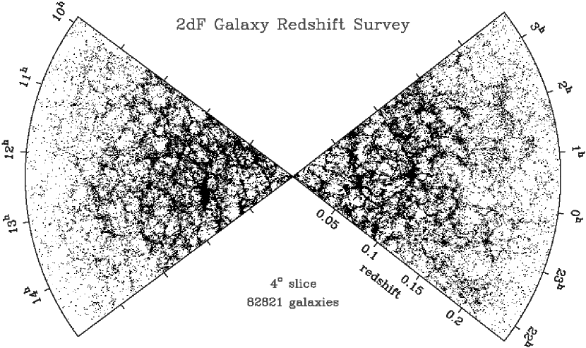
Figure 2: The distribution of galaxies in part of the 2dFGRS: slices $4^{\circ}$ thick, centred at declination $-2.5^{\circ}$ in the NGP and $-27.5^{\circ}$ in the SGP. This magnificently detailed image of large-scale structure provides the basis for measuring the shape of the primordial fluctuation spectrum and hence constraining the matter content of the universe.

The 2dFGRS geometry consists of two contiguous declination strips, plus 100 random 2-degree fields. One strip is in the southern Galactic hemisphere and covers approximately 75^∘$\times$15^∘ centred close to the SGP at ($\alpha,\delta$)=($01^{h}$,$-30^{\circ}$); the other strip is in the northern Galactic hemisphere and covers $75^{\circ}\times 7.5^{\circ}$ centred at ($\alpha,\delta$)=($12.5^{h}$,$+0^{\circ}$). The 100 random fields are spread uniformly over the 7000 deg² region of the APM catalogue in the southern Galactic hemisphere. The sample is limited to be brighter than an extinction-corrected magnitude of $b_{\rm\scriptscriptstyle J}=19.45$ (using the extinction maps of Schlegel et al. 1998). This limit gives a good match between the density on the sky of galaxies and 2dF fibres.

After an extensive period of commissioning of the 2dF instrument, 2dFGRS observing began in earnest in May 1997, and terminated in April 2002. In total, observations were made of 899 fields, yielding redshifts and identifications for 232,529 galaxies, 13976 stars and 172 QSOs, at an overall completeness of 93%. The galaxy redshifts are assigned a quality flag from 1 to 5, where the probability of error is highest at low $Q$. Most analyses are restricted to $Q\geq 3$ galaxies, of which there are currently 221,496. An interim data release took place in July 2001, consisting of approximately 100,000 galaxies (see Colless et al. 2001 for details). A public release of the full photometric and spectroscopic database is scheduled for July 2003. The completed 2dFGRS yields a striking view of the galaxy distribution over large cosmological volumes. This is illustrated in Figure 2, which shows the projection of a subset of the galaxies in the northern and southern strips onto $(\alpha,z)$ slices. This picture is the culmination of decades of effort in the investigation of large-scale structure, and we are fortunate to have this detailed view for the first time.

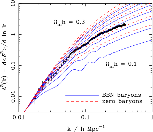
Figure 3: The 2dFGRS redshift-space dimensionless power spectrum, $\Delta^{2}(k)$, estimated according to the FKP procedure. The solid points with error bars show the power estimate. The window function correlates the results at different $k$ values, and also distorts the large-scale shape of the power spectrum An approximate correction for the latter effect has been applied. The solid and dashed lines show various CDM models, all assuming $n=1$. For the case with non-negligible baryon content, a big-bang nucleosynthesis value of $\Omega_{b}h^{2}=0.02$ is assumed, together with $h=0.7$. A good fit is clearly obtained for $\Omega_{m}h\simeq 0.2$. Note that the observed power at large $k$ will be boosted by nonlinear effects, but damped by small-scale random peculiar velocities. It appears that these two effects very nearly cancel, but model fitting is generally performed only at $k<0.15{\,h\,\rm Mpc^{-1}}$ in order to avoid these complications.

2.2 The 2dFGRS power spectrum

Perhaps the key aim of the 2dFGRS was to perform an accurate measurement of the 3D clustering power spectrum, in order to improve on the APM result, which was deduced by deprojection of angular clustering (Baugh & Efstathiou 1993, 1994). The results of this direct estimation of the 3D power spectrum are shown in Figure 3 (Percival et al. 2001). This power-spectrum estimate uses the FFT-based approach of Feldman, Kaiser & Peacock (1994; FKP), and needs to be interpreted with care. Firstly, it is a raw redshift-space estimate, so that the power beyond $k\simeq 0.2{\,h\,\rm Mpc^{-1}}$ is severely damped by smearing due to peculiar velocities, as well as being affected by nonlinear evolution. Finally, the FKP estimator yields the true power convolved with the window function. This modifies the power significantly at large scales (roughly a 20% correction). An approximate correction for this has been made in Figure 3.

Figure 4: Likelihood contours for the best-fit linear CDM fit to the 2dFGRS power spectrum over the region $0.02<k<0.15$. Contours are plotted at the usual positions for one-parameter confidence of 68%, and two-parameter confidence of 68%, 95% and 99% (i.e. $-2\ln({\cal L}/{\cal L_{\rm max}})=1,2.3,6.0,9.2$). We have marginalized over the missing free parameters ($h$ and the power spectrum amplitude). A prior on $h$ of $h=0.7\pm 10\%$ was assumed. This result is compared to estimates from X-ray cluster analysis (Evrard 1997) and big-bang nucleosynthesis (Burles et al. 2001). The second panel shows the 2dFGRS data compared with the two preferred models from the Maximum Likelihood fits convolved with the window function (solid lines). The unconvolved models are also shown (dashed lines). The $\Omega_{m}h\simeq 0.6$, $\Omega_{b}/\Omega_{m}=0.42$, $h=0.7$ model has the higher bump at $k\simeq 0.05{\,h\,\rm Mpc^{-1}}$. The smoother $\Omega_{m}h\simeq 0.20$, $\Omega_{b}/\Omega_{m}=0.15$, $h=0.7$ model is a better fit to the data because of the overall shape. A preliminary analysis of the complete final 2dFGRS sample yields a slightly smoother spectrum than the results shown here (from Percival et al. 2001), so that the high-baryon solution becomes disfavoured.

2.3 CDM model fitting

The fundamental assumption is that, on large scales, linear biasing applies, so that the nonlinear galaxy power spectrum in redshift space has a shape identical to that of linear theory in real space. This assumption is valid for $k<0.15{\,h\,\rm Mpc^{-1}}$; the detailed justification comes from analyzing realistic mock data derived from $N$-body simulations (Cole et al. 1998). The free parameters in fitting CDM models are thus the primordial spectral index, $n$, the Hubble parameter, $h$, the total matter density, $\Omega_{m}$, and the baryon fraction, $\Omega_{b}/\Omega_{m}$. Note that the vacuum energy does not affect the constraints. Initially, we show results assuming $n=1$; this assumption is relaxed later.

An accurate model comparison requires the full covariance matrix of the data, because the convolving effect of the window function causes the power at adjacent $k$ values to be correlated. This covariance matrix was estimated by applying the survey window to a library of Gaussian realisations of linear density fields, and checked against a set of mock catalogues. It is now possible to explore the space of CDM models, and likelihood contours in $\Omega_{b}/\Omega_{m}$ versus $\Omega_{m}h$ are shown in Figure 4. At each point in this surface we have marginalized by integrating the likelihood surface over the two free parameters, $h$ and the power spectrum amplitude. We have added a Gaussian prior $h=0.7\pm 10\%$, representing external constraints such as the HST key project (Freedman et al. 2001); this has only a minor effect on the results.

Figure 4a shows that there is a degeneracy between $\Omega_{m}h$ and the baryonic fraction $\Omega_{b}/\Omega_{m}$. However, there are two local maxima in the likelihood, one with $\Omega_{m}h\simeq 0.2$ and $\sim 20\%$ baryons, plus a secondary solution $\Omega_{m}h\simeq 0.6$ and $\sim 40\%$ baryons. The high-density model can be rejected through a variety of arguments, and the preferred solution is

$$\Omega_{m}h=0.20\pm 0.03;\quad\quad\Omega_{b}/\Omega_{m}=0.15\pm 0.07.$$ (6)

The 2dFGRS data are compared to the best-fit linear power spectra convolved with the window function in Figure 4b. The low-density model fits the overall shape of the spectrum with relatively small ‘wiggles’, while the solution at $\Omega_{m}h\simeq 0.6$ provides a better fit to the bump at $k\simeq 0.065{\,h\,\rm Mpc^{-1}}$, but fits the overall shape less well. A preliminary analysis of $P(k)$ from the full final dataset shows that $P(k)$ becomes smoother: the high-baryon solution becomes disfavoured, and the uncertainties narrow slightly around the lower-density solution: $\Omega_{m}h=0.18\pm 0.02$; $\Omega_{b}/\Omega_{m}=0.17\pm 0.06$.

It is interesting to compare these conclusions with other constraints. These are shown on Figure 4, assuming $h=0.7\pm 10\%$. Latest estimates of the Deuterium to Hydrogen ratio in QSO spectra combined with big-bang nucleosynthesis theory predict $\Omega_{b}h^{2}=0.020\pm 0.001$ (Burles et al. 2001), which translates to the shown locus of $f_{\rm\scriptscriptstyle B}$ vs $\Omega_{m}h$. X-ray cluster analysis predicts a baryon fraction $\Omega_{b}/\Omega_{m}=0.127\pm 0.017$ (Evrard 1997) which is within $1\sigma$ of our value. These loci intersect very close to our preferred model.

Perhaps the main point to emphasise here is that the 2dFGRS results are not greatly sensitive to the assumed tilt of the primordial spectrum. As discussed below, CMB data show that $n=1$ is a very good approximation; in any case, very substantial tilts ($n\simeq 0.8$) are required to alter the conclusions significantly.

2.4 Robustness of results

The main residual worry about accepting the above conclusions is probably whether the assumption of linear bias can really be valid. In general, concentration towards higher-density regions both raises the amplitude of clustering, but also steepens the correlations, so that bias is largest on small scales. A simple model that illustrates this is to assume that the density field is a lognormal process. A nonlinear transformation $\rho\rightarrow\rho^{b}$ then gives a correlation function $1+\xi\rightarrow(1+\xi)^{b^{2}}$ (Mann, Peacock & Heavens 1998). We need to be clear of the regime in which the bias depends on scale.

One way in which this issue can be studied is to consider subsamples with very different degrees of bias. Colour information has recently been added to the 2dFGRS database using SuperCosmos scans of the UKST red plates (Hambly et al. 2001), and a division at rest-frame photographic $B-R=0.85$ nicely separates ellipticals from spirals. Figure 5 shows the power spectra for the 2dFGRS divided in this way. The shapes are almost identical (perhaps not so surprising, since the cosmic variance effects are closely correlated in these co-spatial samples). However, what is impressive is that the relative bias is almost precisely independent of scale, even though the red subset is rather strongly biased relative to the blue subset (relative $b\simeq 1.4$). This provides some reassurance that the large-scale $P(k)$ reflects the underlying properties of the dark matter, rather than depending on the particular class of galaxies used to measure it.

Figure 5: The power spectra of red galaxies (filled circles) and blue galaxies (open circles), divided at photographic $B-R=0.85$. The shapes are strikingly similar, and the square root of the ratio yields the right-hand panel: the relative bias in redshift space of red and blue galaxies. The error bars are obtained by a jack-knife analysis. The relative bias is consistent with a constant value of 1.4 over the range used for fitting of the power-spectrum data ($0.015<k<0.15{\,h\,\rm Mpc^{-1}}$).

3 Combination with the CMB and cosmological parameters

3.1 Parameter degeneracies

The 2dFGRS power spectrum contains important information about the key parameters of the cosmological model, but we have seen that additional assumptions are needed, in particular the values of $n$ and $h$. Observations of CMB anisotropies can in principle measure most of the cosmological parameters, and combination with the 2dFGRS can lift most of the degeneracies inherent in the CMB-only analysis. It is therefore of interest to see what emerges from a joint analysis. These issues are discussed in Efstathiou et al. (2002). The CMB data alone contain two important degeneracies: the ‘geometrical’ and ‘tensor’ degeneracies.

Geometrical degeneracy In the former case, one can evade the commonly-stated CMB conclusion that the universe is flat, by adjusting both $\Lambda$ and $h$ to extreme values (Zaldarriaga et al. 1997; Bond et al. 1997; Efstathiou & Bond 1999). The normal flatness argument takes the comoving horizon size at last scattering

$$D_{\rm\scriptscriptstyle LS}=\frac{2c}{\Omega_{m}^{1/2}H_{0}}\,(1+z_{\rm\scriptscriptstyle LS})^{-1/2}\simeq 184(\Omega_{m}h^{2})^{-1/2}\;{\rm Mpc}$$ (7)

and divides it by the present-day horizon size for a zero-$\Lambda$ universe,

$$D_{\rm\scriptscriptstyle H}=\frac{2c}{\Omega_{m}H_{0}},$$ (8)

to yield a main characteristic angle that scales as $\Omega_{m}^{1/2}$. Large curvature (i.e. low $\Omega_{m}$) is ruled out because the main peak in the CMB power spectrum is not seen at very small angles. However, introducing vacuum energy changes the conclusion. If we take a family of models with fixed initial perturbation spectra, fixed physical densities $\omega_{m}\equiv\Omega_{m}h^{2}$, $\omega_{b}\equiv\Omega_{b}h^{2}$, and vary both $\Omega_{v}$ and the curvature to keep a fixed value of the angular size distance to last scattering, then the resulting CMB power spectra are identical (except for the Integrated Sachs-Wolfe effect at very low multipoles, and second-order effects at high $\ell$). This degeneracy occurs because the physical densities control the structure of the perturbations in physical Mpc at last scattering, while curvature, $\Omega_{v}$ and $\Omega_{m}$ govern the proportionality between length at last scattering and observed angle. In order to break the degeneracy, additional information is needed. This could be in the form of external data on the Hubble constant, but the most elegant approach is to add the 2dFGRS data, so that conclusions are based only on the shapes of power spectra. Efstathiou et al. (2002) show that doing this yields a total density ($|\Omega-1|<0.05$) at 95% confidence. We can therefore be confident that the universe is very nearly flat; hereafter it will be assumed that this is exactly true.

Tensor degeneracy The next most critical question for the CMB is whether the temperature fluctuations are scalar-mode only, or whether there could be a significant tensor signal. The tensor modes lack acoustic peaks, so they reduce the relative amplitude of the main peak at $\ell=220$. A model with a large tensor component can however be made to resemble a zero-tensor model by applying a large blue tilt ($n>1$) and a high baryon content. Efstathiou et al. (2002) show that adding the 2dFGRS data weakens this degeneracy, but does not completely remove it. This is reasonable, since the 2dFGRS data alone constrain the baryon content weakly.

The importance of tensors will of course be one of the key questions for cosmology over the next several years, but it is interesting to consider the limit in which these are negligible. In this case, the standard model for structure formation contains a vector of only 6 parameters: ${\bf p}=(n_{s},\Omega_{m},\Omega_{b},h,Q,\tau)$. Of these, the optical depth to last scattering, $\tau$, is almost entirely degenerate with the normalization, $Q$. The remaining four parameters are pinned down very precisely: using a compilation of pre-WMAP CMB data plus the 2dFRGS power spectrum, Percival et al. (2002) obtained

$$(n_{s},\Omega_{c},\Omega_{b},h)=(0.963\pm 0.042,0.115\pm 0.009,0.021\pm 0.002,0.665\pm 0.047),$$ (9)

or an overall density parameter of $\Omega_{m}=0.313\pm 0.055$.

It is remarkable how well these figures agree with completely independent determinations: $h=0.72\pm 0.08$ from the HST key project (Mould et al. 2000; Freedman et al. 2001); $\Omega_{b}h^{2}=0.020\pm 0.001$ (Burles et al. 2001). This gives confidence that the tensor component must indeed be sub-dominant. For further details of this analysis, see Percival et al. (2002).

3.2 The horizon angle degeneracy

For flat models, there is a degeneracy that is related (but not identical) to the geometrical degeneracy, being very closely related to the location of the acoustic peaks. The angular scale of these peaks depends on the ratio between the horizon size at last scattering and the present-day horizon size for flat models:

$$\theta_{\rm\scriptscriptstyle H}=D_{\rm\scriptscriptstyle H}(z_{\rm\scriptscriptstyle LS})/D_{\rm\scriptscriptstyle H}(z=0);\quad\quad D_{\rm\scriptscriptstyle H}(z=0)=\frac{2c}{H_{0}}\Omega_{m}^{-0.4}.$$ (10)

(using the approximation of Vittorio & Silk 1985). This yields an angle scaling as $\Omega_{m}^{-0.1}$, so that the scale of the acoustic peaks is apparently almost independent of the main parameters.

However, this argument is not complete because the earlier expression for $D_{\rm\scriptscriptstyle H}(z_{\rm\scriptscriptstyle LS})$ assumes that the universe is completely matter dominated at last scattering. The comoving sound horizon size at last scattering is defined by (e.g. Hu & Sugiyama 1995)

$$D_{\rm\scriptscriptstyle S}(z_{\rm\scriptscriptstyle LS})\equiv\frac{1}{H_{0}\Omega_{m}^{1/2}}\int_{0}^{a_{\rm\scriptscriptstyle LS}}\frac{c_{\rm\scriptscriptstyle S}}{(a+a_{\rm eq})^{1/2}}\,da$$ (11)

where vacuum energy is neglected at these high redshifts; the expansion factor $a\equiv(1+z)^{-1}$ and $a_{\rm\scriptscriptstyle LS},a_{\rm eq}$ are the values at last scattering and matter-radiation equality respectively. In practice, $z_{\rm\scriptscriptstyle LS}\simeq 1100$ independent of the matter and baryon densities, and $c_{\rm\scriptscriptstyle S}$ is fixed by $\Omega_{b}$. Thus the main effect is that $a_{\rm eq}$ depends on $\Omega_{m}$. Dividing by $D_{\rm\scriptscriptstyle H}(z=0)$ therefore gives the angle subtended today by the light horizon as

$$\theta_{\rm\scriptscriptstyle H}\simeq\frac{\Omega_{m}^{-0.1}}{\sqrt{1+z_{\rm\scriptscriptstyle LS}}}\left[\sqrt{1+\frac{a_{\rm eq}}{a_{\rm\scriptscriptstyle LS}}}-\sqrt{\frac{a_{\rm eq}}{a_{\rm\scriptscriptstyle LS}}}\,\right],$$ (12)

where $z_{\rm\scriptscriptstyle LS}=1100$ and $a_{\rm eq}=(23900\,\omega_{m})^{-1}$. This remarkably simple result captures most of the parameter dependence of CMB peak locations within flat $\Lambda$CDM models. Differentiating this equation near a fiducial $\omega_{m}=0.147$ gives

$$\left.\frac{\partial\ln\theta_{\rm\scriptscriptstyle H}}{\partial\ln\Omega_{m}}\right|_{\omega_{m}}=-0.1;\quad\quad\left.\frac{\partial\ln\theta_{\rm\scriptscriptstyle H}}{\partial\ln\omega_{m}}\right|_{\Omega_{m}}=\frac{1}{2}\left(1+\frac{a_{\rm\scriptscriptstyle LS}}{a_{\rm eq}}\right)^{-1/2}=+0.24,$$ (13)

in good agreement with the numerical derivatives in Eq. (A15) of Hu et al. (2001).

Thus for moderate variations from a ‘fiducial’ model, the CMB peak multipole number scales approximately as $\ell_{\rm peak}\propto\Omega_{m}^{-0.14}h^{-0.48}$, i.e. the condition for constant CMB peak location is well approximated as

$$\Omega_{m}h^{3.4}={\rm constant}.$$ (14)

However, information about the peak heights does alter this degeneracy slightly; the relative peak heights are preserved at constant $\Omega_{m}$, hence the actual likelihood ridge is a ‘compromise’ between constant peak location (constant $\Omega_{m}h^{3.4}$) and constant relative heights (constant $\Omega_{m}h^{2}$); the peak locations have more weight in this compromise, leading to a likelihood ridge along approximately $\Omega_{m}h^{3.0}\simeq{\rm const}$ (Percival et al. 2002). It is now clear how LSS data combines with the CMB: $\Omega_{m}h^{3.4}$ is measured to very high accuracy already, and Percival et al. deduced $\Omega_{m}h^{3.4}=0.078$ with an error of about 6% using pre-WMAP CMB data. The first-year WMAP results in fact prefer $\Omega_{m}h^{3.4}=0.084$ (Spergel et al. 2003); the slight increase arises because WMAP indicates that previous datasets around the peak were on average calibrated low.

In any case, the dominant error in $\Omega_{m}$ and $h$ depends on what one chooses to add to the $\Omega_{m}h^{3.4}$ figure. The best approach given current knowledge is probably to combine the WMAP $\Omega_{m}h^{3.4}=0.084$ with the updated 2dFGRS $\Omega_{m}h=0.18\pm 0.02$: this yields $\Omega_{m}=0.25\pm 15\%$ and $h=0.73\pm 5\%$.

3.3 Matter fluctuation amplitude and bias

The above conclusions were obtained by considering the shapes of the CMB and galaxy power spectra. However, it is also of great interest to consider the amplitude of mass fluctuations, since a comparison with the galaxy power spectrum allows us to infer the degree of bias directly. This analysis was performed by Lahav et al. (2002). Given assumed values for the cosmological parameters, the present-day linear normalization of the mass spectrum (e.g. $\sigma_{8}$) can be inferred. It is convenient to define a corresponding measure for the galaxies, $\sigma_{8{\rm g}}$, such that we can express the bias parameter as

$$b=\frac{\sigma_{8{\rm g}}}{\sigma_{8{\rm m}}}.$$ (15)

In practice, we define $\sigma_{8{\rm g}}$ to be the value required to fit a CDM model to the power-spectrum data on linear scales ($0.02<k<0.15{\,h\,\rm Mpc^{-1}}$). The amplitude of 2dFGRS galaxies in real space estimated by Lahav et al. (2002) is $\smash{\sigma_{8{\rm g}}^{R}}(L^{*})=0.76$, with a negligibly small random error. This assumes no evolution in $\smash{\sigma_{8{\rm g}}}$, plus the luminosity dependence of clustering measured by Norberg et al. (2001).

The value of $\sigma_{8}$ for the dark matter can be deduced from the CMB fits. Percival et al. (2002) obtain

$$\sigma_{8}\exp(-\tau)=0.72\pm 0.04,$$ (16)

where the quoted error includes both data errors and theory uncertainty. The WMAP value here is almost identical: $\sigma_{8}\exp(-\tau)=0.71$, but no error is quoted (Spergel et al. 2003). The unsatisfactory feature is the degeneracy with the optical depth to last scattering. For reionization at $z=8$, we would have $\tau\simeq 0.05$; it is not expected theoretically that $\tau$ can be hugely larger, and popular models would place reionization between $z=10$ and $z=15$, or $\tau\simeq 0.1$ (e.g. Loeb & Barkana 2001). One of the many impressive aspects of the WMAP results is that they are able to infer $\tau=0.17\pm 0.04$ from large-scale polarization. Taken at face value, $\tau=0.17$ would argue for reionization at $z=20$, but the error means that more conventional figures are far from being ruled out. Taking all this together, it seems reasonable to assume that the true value of $\sigma_{8}$ is within a few % of 0.80. Given the 2dFGRS figure of $\smash{\sigma_{8{\rm g}}^{R}}=0.76$, this implies that $L^{*}$ galaxies are very nearly exactly unbiased. Since there are substantial variations in the clustering amplitude with galaxy type, this outcome must be something of a coincidence.

Finally, this conclusion of near-unity bias was reinforced in a completely independent way, by using the measurements of the bispectrum of galaxies in the 2dFGRS (Verde et al. 2002). As it is based on three-point correlations, this statistic is sensitive to the filamentary nature of the galaxy distribution – which is a signature of nonlinear evolution. One can therefore split the degeneracy between the amplitude of dark-matter fluctuations and the amount of bias.

4 Less-standard ingredients

4.1 Limits to the neutrino mass

Even though a CDM-dominated universe matches the data very well, there are many plausible variations to consider. Probably the most interesting is the neutrino mass: experimental data mean that at least one neutrino must have a mass of $\mathrel{\lower 2.58334pt\hbox{$\buildrel{\textstyle>}\over{\scriptstyle\sim}$}}0.05$ eV, so that $\Omega_{\nu}\mathrel{\lower 2.58334pt\hbox{$\buildrel{\textstyle>}\over{\scriptstyle\sim}$}}10^{-3}$ – the same order of magnitude as stellar mass.

Figure 6: Results from Elgaroy et al. (2002), who considered constraints on the neutrino mass from 2dFGRS. The first panel shows Power spectra for $\Omega_{\nu}=0$ (solid line), $\Omega_{\nu}=0.01$ (dashed line), and $\Omega_{\nu}=0.05$ (dot-dashed line) with amplitudes fitted to the 2dFGRS power spectrum data (vertical bars). Other parameters are fixed at $\Omega_{\rm m}=0.3$, $\Omega_{\Lambda}=0.7$, $h=0.7$, $\Omega_{\rm b}h^{2}=0.02$. The vertical dashed lines limit the range in $k$ used in the fits. The second panel shows 68% (solid line), 95% (dashed line) and 99% (dotted line) confidence contours in the plane of $f_{\nu}\equiv\Omega_{\nu}/\Omega_{\rm m}$ and $\Gamma\equiv\Omega_{\rm m}h$, with marginalization over $h$ and $\Omega_{\rm b}h^{2}$ using Gaussian priors.

As explained in Section 1, a non-zero neutrino mass can lead to relatively enhanced large-scale power, beyond the neutrino free-streaming scale. This is illustrated in Figure 6, taken from Elgaroy et al. (2002). Broadly speaking, allowing a significant neutrino mass changes the spectrum in a way that resembles lower density, so there is a near-degeneracy between neutrino mass fraction and $\Omega_{m}h$ (Figure 6b). A limit on the neutrino fraction thus requires a prior on $\Omega_{m}h$. Based on the cluster baryon fraction plus BBN, Elgaroy et al. adopt $\Omega_{m}<0.5$; together with the HST Hubble constant, this yields a marginalized 95% limit of $f_{\nu}<0.13$, or $m_{\nu}<1.8$ eV. Note that this is the sum of the eigenvalues of the mass matrix: given neutrino oscillation results, the only way a cosmologically significant density can arise is via a nearly degenerate hierarchy, so this allows us to deduce $m_{\nu}<0.6$ eV for any one species.

4.2 The equation of state of the vacuum

So far, we have assumed that the vacuum energy is exactly a classical $\Lambda$, or at any rate indistinguishable from one. This is a highly reasonable prior: there is no reason for the asymptotic value of any potential to go exactly to zero, so one always needs to solve the classical cosmological constant problem – for which probably the only reasonable explanation is an anthropic one (e.g. Vilenkin 2001). Therefore, dynamical provision of $w\equiv p_{v}/\rho_{v}\neq-1$ is not needed. Nevertheless, one can readily take an empirical approach to $w$ (treated as a constant for a frst approach).

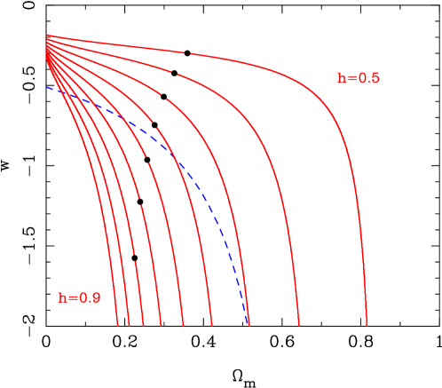
Figure 7: The $\Omega_{m}h^{3.4}$ degeneracy for flat models gives an almost exact value of $\Omega_{m}$ from the CMB is $h$ is known, assuming the vacuum to be effectively a classical $\Lambda$ ($w=-1$). If $w$ is allowed to vary, this becomes a locus on the $(\Omega_{m},w)$ plane (similar to the locus for best-fitting flat models from the SNe, showed dotted). Solid circles show values of $\Omega_{m}h$ that satisfy the updated 2dFGRS constraint of 0.18 (suppressing error bars).

Figure 7 shows a simplified approach to this, plotting the locus on $(w,\Omega_{m})$ space that is required for a given value of $h$ if the location of the main CMB acoustic peak is known exactly. For $h\simeq 0.7$, this is very similar to the locus derived from the SN Hubble diagram (Garnavich et al. 1998). The solid circles show the updated 2dFGRS constraint of $\Omega_{m}h=0.18$. In order to match the data with $w$ closer to zero, $\Omega_{m}$ must increase and $h$ must decrease. The latter trend means that the HST Hubble constant sets an upper limit to $w$ of about $-0.54$ (Percival et al. 2002). This is very similar to the SNe constraint of Garnavich et al. (1998), so the combined limit is already close to $w<-0.8$. The vacuum energy is indeed looking rather similar to $\Lambda$.

4.3 The total relativistic density

Finally, an interesting aspect of Figure 7 is that it reminds us of history. When the COBE detection was announced in 1992, a popular model was ‘standard’ CDM with $\Omega_{m}=1$, $h=0.5$. As we see, this comes close to fitting the CMB data, and such a model is not unattractive in some ways. Can we be sure it is ruled out? Leaving aside the SNe data, one might think to evade the 2dFGRS constraint by altering the total relativistic content of the universe (for example, by the decay of a heavy neutrino after nucleosynthesis). Since 2dFGRS measures the horizon at matter-radiation equality, this will be changed. If the radiation density is arbitrarily boosted by a factor $X$, the constraint from LSS becomes

$$(\Omega_{m}h)_{\rm apparent}=X^{-1/2}(\Omega_{m}h)_{\rm true}.$$ (17)

Therefore $X\simeq 8$ is required to allow an Einstein–de Sitter universe.

However, this argument fails, because it does not take into account the effect of the extra radiation on the CMB. As argued above, the location of the acoustic peaks depends on $a_{\rm eq}$, which depends on $\omega_{m}$. However, if we change the radiation content, then what matters is $\omega_{m}/X$. Thus, the CMB peak constraint now reads

$$\Omega_{m}^{-0.1}(\omega_{m}/X)^{0.24}={\rm constant};$$ (18)

when combining LSS and CMB, everything is as before except that the effective Hubble parameter is $h/X^{1/2}$. Thus, a model with $\Omega_{m}=1$ but boosted radiation would only fit the CMB with $h\simeq 0.5\sqrt{8}\simeq 1.4$, and the attractiveness of a low age is lost. In any case, combining LSS and CMB would give the same $\Omega_{m}\simeq 0.3$ independent of $X$, so it is impossible to save models with $\Omega_{m}=1$ by this route.

Finally, it is interesting to invert this argument. Since Percival et al. (2002) obtain an effective $h$ of $0.665\pm 0.047$ and Freedman et al. (2001) measure $h=0.72\pm 0.08$, we deduce

$$1.68X=1.82\pm 0.24.$$ (19)

This convincingly rules out the $1.68X=1$ that would apply if the universe contained only photons, and amounts to a detection of the neutrino background. In terms of the number of neutrino species, this is $N_{\nu}=3.6\pm 1.1$. A more precise result is of course obtained from primordial nucleosynthesis, but this applies at a much later epoch, thus constraining models with decaying particles.

5 Conclusions

The beautiful data on the large-scale structure of the universe revealed in particular by the 2dF Galaxy Redshift Survey combine with the incredible recent progress in CMB data to show spectacularly good agreement with a ‘standard model’ for structure formation. This consists of a scalar-mode adiabatic CDM universe with scale-invariant fluctuations. Measuring the exact parameters of this model is rendered difficult by the intrinsic degeneracies of the structure-formation process, but progress is being made. The most recent data yield $\Omega_{m}=0.25\pm 15\%$ and $h=0.73\pm 5\%$; these figures accord well with independent constraints, and it is very hard to believe that they are incorrect.

Allowing extra degrees of freedom, such as massive neutrinos, vacuum equation of state $w\neq 1$, or extra relativistic content worsens the agreement with independent constraints on $h$ and $\Omega_{m}$. This both supports the simplest picture and allows us to set interesting limits on these non-standard ingredients.

For the future, we can look with anticipation to meaningful tests of inflation: the current data are consistent with $n=1$ to an error of $\pm 0.03$. Once this is halved, plausible levels of tilt will come within our sensitivity. The tensor fraction is a less clear target, but the motivation to improve on the current weak upper limits will remain strong.

It should of course not be forgotten that the large-scale structure we measure locally consists of galaxies. In this paper, the physics of galaxy formation has been sadly ignored, but this will be the increasing focus of LSS studies: not just the global parameters of the universe, but the detailed understanding of how the complex structures around us formed.

References

Baugh C.M., Efstathiou G., 1993, MNRAS, 265, 145

Baugh C.M., Efstathiou G., 1994, MNRAS, 267, 323

Bond J.R., Szalay A., 1983, ApJ, 274, 443

Bond J.R., Efstathiou G., Tegmark M., 1997, MNRAS, 291, L33

Bucher M., Moodley K., Turok, N., 2002, Phys. Rev. D, 66, 023528

Burles S., Nollett K.M., Turner M.S., 2001, ApJ, 552, L1

Cole S., Hatton S., Weinberg D.H., Frenk C.S., 1998, MNRAS, 300, 945

Colless M. et al., 2001, MNRAS, 328, 1039

Efstathiou G., Bond J.R., 1999, MNRAS, 304, 75

Efstathiou G. et al., 2002, MNRAS, 330, L29

Elgaroy O. et al., 2002, Phys. Rev. Lett., 89, 061301

Evrard A., 1997, MNRAS, 292, 289

Feldman H.A., Kaiser N., Peacock J.A., 1994, ApJ, 426, 23

Freedman W.L. et al., 2001, ApJ, 553, 47

Garnavich P.M. et al., 1998, ApJ, 509, 74

Goldberg D.M., Strauss M., 1998, ApJ, 495, 29

Hambly N.C., Irwin M.J., MacGillivray H.T., 2001, MNRAS, 326 1295

Hu W., Sugiyama N., 1995, ApJ, 444, 489

Hu W., Fukugita M., Zaldarriaga M., Tegmark M., 2001, ApJ, 549, 669

Lahav O. et al., 2002, MNRAS, 333, 961

Lewis I.J. et al., 2002, MNRAS, 333, 279

Loeb A., Barkana R., 2001, ARAA, 39, 19

Maddox S.J., Efstathiou G., Sutherland W.J., Loveday J., 1990a, MNRAS, 242, 43p

Maddox S.J., Sutherland W.J., Efstathiou G., Loveday J., 1990b, MNRAS, 243, 692

Maddox S.J., Efstathiou G., Sutherland W.J., 1990c, MNRAS, 246, 433

Mann R.G., Peacock J.A., Heavens A.F., 1998, MNRAS, 293, 209

Meiksin A.A., White M., Peacock J.A., 1999, MNRAS, 304, 851

Mould J.R. et al., 2000, ApJ, 529, 786

Narayanan V.K., Spergel D.N., Davé R., Ma C.-P., 2000, ApJ, 543, L103

Norberg P. et al., 2001, MNRAS, 328, 64

Percival W.J. et al., 2001, MNRAS, 327, 1297

Percival W.J. et al., 2002, MNRAS, 337, 1068

Schlegel D.J., Finkbeiner D.P., Davis M., 1998, ApJ, 500, 525

Seljak U., Zaldarriaga M., 1996, ApJ, 469, 437

Spergel D.N. et al., 2003, astro-ph/0302209

Stoughton C.L. et al., 2002, AJ, 123, 485

Verde L. et al., 2002, MNRAS, 335, 432

Vilenkin A., 2001, hep-th/0106083

Vittorio N., Silk J., 1985, ApJ, 297, L1

Zaldarriaga M., Spergel, D., Seljak U., 1997, ApJ, 488, 1