GRB Formation Rates inferred from the Spectral Peak Energy – Luminosity Relation

Abstract

We investigate the GRB formation rate based on the relation between the spectral peak energy ($E_{p}$) and the isotropic luminosity. The $E_{p}$–luminosity relation covers the energy range of 50 – 2000 keV and the luminosity range of $10^{50}$–$10^{54}~{}{\rm erg~{}s^{-1}}$, respectively. We find that the relation is considerably tighter than similar relations suggested previously. Using $E_{p}$–luminosity relation, we estimate the luminosity and the redshift of 684 GRBs with the unknown distances and derive the GRB formation rate as a function of the redshift. For $0\leq z\leq 2$ , the GRB formation rate is well correlated with the star formation rate while it increases monotonously from $z\sim 2$ out to $z\sim 12$. This behavior is consistent with the results of previous works using the lag–luminosity relation or the variability–luminosity relation.

1 Introduction

Many ground based telescopes have tried to detect optical afterglows of GRBs and to measure their redshifts by using the spectral absorption and/or emission lines of the interstellar matter in the host galaxy. However, the number of GRBs with measured redshift is only a fraction of all GRBs detected with BATSE, BeppoSAX, HETE-II and INTEGRAL satellites; we have still only about 30 GRBs with the known redshifts. The most of them occur at the cosmological distance, and the current record holder is GRB 000131 at $z=4.5$ (Andersen et al., 2000). According to the brightness distribution of GRBs with the known redshifts, the above satellites should have already detected much more distant GRBs, such as at $z\sim 20$ (Band, 2003). If we can establish a method for estimating the intrinsic brightness from the characteristics of the prompt gamma-ray emission, we can use the brightness of the GRB as a lighthouse to determine the unknown redshifts of majority of GRBs, which enables us to explore the early universe out to $z\sim 20$.

Using the geometrical corrections of the collimated jets, Frail et al. (2001) and Bloom et al. (2003) revealed that the bolometric energies released in the prompt emission are tightly clustering around the standard energy of $\sim 1\times 10^{51}~{}{\rm erg}$. Thus, the explosion energy of GRBs can be used as a standard candle as the supernovae. However, the apparent brightness of GRBs strongly depends on the jet opening angle and the viewing angle. To use the GRB as the standard candle, we need to correct such effects.

Several authors tried to establish a method for estimating the isotropic luminosity from the observed GRB properties. Using the lightcurves of the prompt gamma-ray emissions, some pioneering works have been done; the variability–luminosity relation reported by Fenimore & Ramirez-Ruiz (2000), which indicates that the variable GRBs are much brighter than the smooth ones. The spectral time-lag, which is the interval of the peak arrival times between two different energy bands, also correlates with the isotropic luminosity (Norris et al., 2000). These properties based on the time-series data might be due to the effect of the viewing angle from the GRB jet (e.g., Ioka & Nakamura, 2001; Norris, 2002; Murakami et al., 2003).

On the other hand, based on the spectral analyses with the K-correction (Bloom et al., 2001), Amati et al. (2002) found the correlation between the isotropic-equivalent energy radiated in GRBs and the peak energies $E_{p}$, which is the energy at the peak of $\nu F_{\nu}$ spectrum. Atteia (2003) suggested a possibility of the empirical redshift indicator, which is based on the $E_{p}$ and the arrival number of photons.

Applying these luminosity indicators to the GRBs with the unknown redshifts, their redshifts can be estimated from the apparent gamma-ray brightness. As a natural application of the obtained redshift distribution, the GRB formation rates are discussed by several authors (e.g., Fenimore & Ramirez-Ruiz, 2000; Norris et al., 2000; Schaefer et al., 2001; Lloyd-Ronning et al., 2002; Murakami et al., 2003). Especially, using mathematically rigid method (Efron & Petrosian, 1992; Petrosian, 1993; Maloney & Petrosian, 1999), Lloyd-Ronning et al. (2002) have estimated the GRB formation rates from the variability–luminosity relation. These works give basically the same results; the GRB formation rate rapidly increases with the redshift at $0\lesssim z\lesssim 2$, and it keeps on rising up to higher redshift ($z\sim 12$). The GRB formation rate did not decrease with $z$ in contrast with the star formation rates (SFRs) measured in UV, optical and infrared band (e.g., Madau et al., 1996; Barger et al., 2000; Stanway et al., 2003).

In this paper, we establish a new calibration formula of the redshift based on the $E_{p}$–luminosity relation of the brightest peak of the prompt gamma-ray emission from 9 GRBs with the known redshifts. Importantly, the uncertainty of our formula is much less than those of the previous works (lag, variability) as shown in section 3. Applying the obtained calibration, in section 4, we estimate the redshifts of 684 GRBs with the unknown redshifts. We then demonstrate the GRB formation rate out to $z\sim 12$ and the luminosity evolution using the non-parametric method (Efron & Petrosian, 1992; Petrosian, 1993; Maloney & Petrosian, 1999; Lloyd-Ronning et al., 2002). We emphasize that the GRB formation rate derived by us is based on the spectral analysis for the first time, and its uncertainty is well controlled in a small level. Throughout the paper, we assume the flat-isotropic universe with $\Omega_{m}=0.32$, $\Omega_{\Lambda}=0.68$ and $H_{0}=72~{}{\rm{km~{}s^{-1}Mpc^{-1}}}$ (Bennett et al., 2003; Spergel et al., 2003).

2 Data Analysis

We used 9 GRBs (970508, 970828, 971214, 980703, 990123, 990506, 990510, 991216, and 000131) in the BATSE archive with the known redshifts, and focused on the brightest peak in each GRB. We performed the spectral analysis with the standard data reduction for each GRB. We subtracted the background spectrum, which was derived from the average spectrum before and after the GRB in the same data set.

We adopted the spectral model of smoothly broken power-law (Band et al., 1993). The model function is described below.

$$N(E)=\left\{\begin{array}[]{ll}A\Bigl{(}\frac{E}{100~{}{\rm keV}}\Bigr{)}^{\alpha}\exp(-\frac{E}{E_{0}}),&\\ A\Bigl{(}\frac{E}{100~{}{\rm keV}}\Bigr{)}^{\beta}\Bigl{(}\frac{(\alpha-\beta)E_{0}}{100~{}{\rm keV}}\Bigr{)}^{\alpha-\beta}\exp(\beta-\alpha),&\\ \end{array}\right.$$ (3)

for $E\leq(\alpha-\beta)E_{0}$ and $E\geq(\alpha-\beta)E_{0}$, respectively. Here, $N(E)$ is in units of $\rm{photons~{}cm^{-2}s^{-1}keV^{-1}}$, and $E_{0}$ is the energy at the spectral break. $\alpha$ and $\beta$ is the low- and high-energy power-law index, respectively. For the case of $\beta<-2$ and $\alpha>-2$, the peak energy can be derived as $E_{p}=(2+\alpha)E_{0}$, which corresponds to the energy at the maximum flux in $\nu F_{\nu}$ spectra. The isotropic luminosity can be calculated with the observed flux as $L=4\pi d_{\rm L}^{2}F_{\gamma}$, where $d_{\rm L}$ and $F_{\gamma}$ are the luminosity distance and the observed energy flux, respectively.

3 $E_{p}$–Luminosity relation

In figure 1, we show the observed isotropic luminosity in units of $10^{52}~{}{\rm{erg~{}s^{-1}}}$ as a function of the peak energy, $E_{p}(1+z)$, in the rest frame of each GRB. For one of our sample (GRB 980703), a lower limit of $E_{p}(1+z)$ is set because the spectral index $\beta>-2$. The results of BeppoSAX reported by Amati et al. (2002) are also plotted in the same figure. Here, we converted their peak fluxes into the same energy range of 30 – 10000 keV in our analysis with their spectral parameters. There is a good positive correlation between the $E_{p}(1+z)$ and the $L$. The linear correlation coefficient including the weighting factors is 0.957 for 15 degree of freedom (17 samples with firm redshift estimates) for the $\log[E_{p}(1+z)]$ and the $\log[L]$. The chance probability is $1.85\times 10^{-9}$. When we adopt the power-law model as the $E_{p}$–luminosity relation, the best-fit function is

$$\frac{L}{10^{52}\ {\rm ergs}}=(4.29\pm 0.15)\times 10^{-5}\biggl{[}\frac{E_{p}(1+z)}{1~{}{\rm keV}}\biggr{]}^{1.94\pm 0.19}$$ (4)

where the uncertainties are 1 $\sigma$ error. This relation agrees well with the standard synchrotron model, $L\propto E_{p}^{2}$ (e.g., Zhang & Mészáros, 2002; Lloyd et al., 2000).

4 Redshift Estimation and GRB Formation Rate

The $E_{p}$–luminosity relation derived in the previous section seems to be much better estimator of the isotropic luminosity compared with the spectral time-lag and the variability of GRBs (Norris et al., 2000; Fenimore & Ramirez-Ruiz, 2000; Schaefer et al., 2001) since the chance probability is extremely low. In this section, using the $E_{p}$–luminosity relation, we try to estimate the isotropic luminosities and the redshifts of the BATSE GRBs with the unknown redshifts.

We first selected about 1000 GRBs in a class of the long duration of $T_{90}>2~{}{\rm sec}$ detected by BATSE, and extracted the brightest pulse in each GRB. We performed the spectral analysis for these peaks with the same method described in section 2. Once we obtained observed energy-flux $F_{\gamma}$ and $E_{p}$ at the observer’s rest frame, we can estimate the redshift with equation (4) and the luminosity distance as a function of the redshift. We could not determine $E_{p}$ for $\sim 5$ % of samples because of $\beta>-2$ within 1 $\sigma$ uncertainty, and excluded them. After setting the flux limit of $F_{\rm limit}=1\times 10^{-7}~{}{\rm erg~{}cm^{-2}s^{-1}}$, which is based on the dimmest one (GRB 970508), on the data set of $(z,L)$ plane, 684 samples are remained. In figure 2, we show the sample distribution in $(z,L)$ plane with the truncation by the flux limit.

The normalized cumulative luminosity function at each redshift bin is also shown in figure 2 . The shape of these luminosity functions are similar to each other, but the break-luminosity seems to increase toward the higher redshift. This indicates that a luminosity evolution is hidden in the $(z,L)$ plane in figure 2. Therefore, we have to remove the effect of the luminosity evolution from the data set before discussing the real luminosity function and the GRB formation rate. This is because the univariate distribution of the redshift and the luminosity can be estimated only when they are independent of each other.

We used the non-parametric method (Lynden-Bell, 1971; Efron & Petrosian, 1992; Petrosian, 1993; Maloney & Petrosian, 1999), which were used for the Quasar samples and first applied to the GRB samples by Lloyd-Ronning et al. (2002). The total luminosity function $\Phi(L,z)$ can be written $\Phi(L,z)=\rho(z)\phi(L/g_{k}(z),\alpha_{s})/g_{k}(z)$ without the loss of generality. Here, each function means the luminosity evolution $g_{k}(z)$, the density evolution $\rho(z)$ and the local luminosity function $\phi(L/g_{k}(z),\alpha_{s})$, respectively. Although the parameter $\alpha_{s}$ represents the shape of the luminosity function, we will ignored the effect of this parameter because the shape of the luminosity function is approximately same as shown in figure 2. We do not mention more about the method, but the details are found in Maloney & Petrosian (1999).

Assuming the functional form of the luminosity evolution as $g_{k}(z)=(1+z)^{k}$, which is also used in Maloney & Petrosian (1999) and Lloyd-Ronning et al. (2002), we convert the data set of $(z,L)$ to $(z,L^{\prime})$, where $L^{\prime}=L/g_{k}(z)$. We search the best value of $k$ giving the independent set of $(z,L^{\prime})$ within the significance of $1~{}\sigma$ error, and it is found to be $g_{k}(z)=(1+z)^{1.85\pm 0.08}$. Once we obtain the independent data set of the $(z,L^{\prime})$, we can generate the cumulative luminosity function $\psi(L^{\prime})$ with a simple formula (see equation (14) of Maloney & Petrosian, 1999). In figure 3, we show the cumulative luminosity function calculated by the formula. This function is approximately described by $\psi(L^{\prime})\propto L^{\prime-0.3}$ for $0.1<L^{\prime}_{52}<1$ and $\psi(L^{\prime})\propto L^{\prime-1.2}$ for $1<L^{\prime}_{52}<50$, where $L^{\prime}_{52}=L^{\prime}/10^{52}\ {\rm ergs}$.

We can also obtain the cumulative number distribution $\psi(z)$ as a function of $z$. The differential form of the function is useful for the purpose of comparison with the star formation rates in other wave bands. We convert $\psi(z)$ into the differential form with the following equation.

$$\rho(z)=\frac{d\psi(z)}{dz}(1+z)\left(\frac{dV(z)}{dz}\right)^{-1}\ ,$$ (5)

where the additional factor of $(1+z)$ comes from the cosmological time dilation, and $dV(z)/dz$ is a differential comoving volume. In figure 4, we show the relative comoving GRB rate $\rho(z)$ in unit proper volume.

5 Discussion

We have investigated the spectral property of the brightest peak of each GRB with the known redshifts, and have found a fine correlation between the peak energy $E_{p}(1+z)$ and the isotropic luminosity. While this correlation against a smaller sample has been pointed out by some authors (e.g., Amati et al., 2002; Atteia, 2003; Schaefer, 2003a, b), we have succeeded in combining the results of BeppoSAX and BATSE to describe equation (4).

Using the new $E_{p}$–luminosity relation, we have estimated the redshifts of 684 GRBs with the unknown redshifts. We found the existence of the luminosity evolution $g_{k}(z)=(1+z)^{1.85\pm 0.08}$ for GRB samples as shown in figure 2. The null-hypothesis of the luminosity evolution is rejected about $9\sigma$ significance. Lloyd-Ronning et al. (2002) also suggest the presence of the luminosity evolution as $g_{k}(z)=(1+z)^{1.4\pm 0.5}$. These two values are consistent with each other. The luminosity evolutions are found in other objects. For example, Caditz & Petrosian (1990) and Maloney & Petrosian (1999) estimated the luminosity evolution of the QSO samples as $g_{k}(z)=(1+z)^{3}$ and $(1+z)^{2.58}$, respectively. Based on the observation of Subaru Deep Field and a photometric redshift estimation for $K^{\prime}$-band selected galaxy samples, Kashikawa et al. (2003) found the strong luminosity evolution in the rest UV band of their galaxies.

The form of the cumulative luminosity function is independent of $z$ except for the break luminosity, which changes with $z$. We propose that figure 3 might include important information on the jets responsible for the prompt $\gamma$-ray emissions and a distribution of their opening angles. Consider an extremely simple model for a uniform jet with an opening half-angle $\theta_{j}$ and a constant geometrically-corrected luminosity $L_{0}$, which is viewed from an angle of $\theta_{v}$. Then, in a crude approximation the luminosity $L$ is given by

$$L=\left\{\begin{array}[]{ll}2L_{0}\theta_{j}^{-2}&{\rm for}\ \ \theta_{v}<\theta_{j}\\ 2L_{0}(\theta_{j}^{6}/\theta_{v}^{8})&{\rm for}\ \ \theta_{v}>\theta_{j}.\\ \end{array}\right.$$ (8)

For the case of $\theta_{v}>\theta_{j}$, $L$ is proportional to $\delta^{4}$, where $\delta=[\gamma(1-\beta\cos\theta_{v})]^{-1}\propto\theta_{v}^{-2}$, so that the luminosity has the dependence of $\theta_{v}^{-8}$ (Ioka & Nakamura, 2001; Yamazaki et al., 2002, 2003). The dependence of $\theta_{j}^{6}$ is determined in order that two functions in equation (8) are continuously connected at $\theta_{v}=\theta_{j}$. We also consider the distribution of $\theta_{j}$ in the form $f(\theta_{j})d\theta_{j}\propto\theta_{j}^{-q}d\theta_{j}$ when $\theta_{{\rm min}}<\theta_{j}<\theta_{{\rm max}}$. Then, easy calculations show that in the case of $q<5/2$, we have

$$N(>L)\propto\left\{\begin{array}[]{ll}L^{-1/4}&{\rm for}\ L<2L_{0}\theta_{{\rm max}}^{-2}\\ L^{(q-3)/2}&{\rm for}\ 2L_{0}\theta_{{\rm max}}^{-2}<L<2L_{0}\theta_{{\rm min}}^{-2}.\end{array}\right.\ .$$ (11)

This is a broken power low with the break luminosity $2L_{0}\theta_{{\rm max}}^{-2}$. Then if $\theta_{{\rm max}}^{-2}L_{0}\propto g_{k}(z)$ with $q=0.6$, we can roughly reproduce figure 3. This suggests that either the maximum opening half angle of the jet decreases or $L_{0}$ increases as a function of the redshift.

This work is the first study to generate the GRB formation rate with $E_{p}$–luminosity relation. The result indicates that the GRB formation rate always increases toward $z\sim 12$. This is consistent with the previous works using the GRB variability (Fenimore & Ramirez-Ruiz, 2000; Lloyd-Ronning et al., 2002) and the spectral time-lag (Norris et al., 2000; Schaefer et al., 2001; Murakami et al., 2003). Quantitatively, GRB formation rate is proportional to $(1+z)^{5-6}$ for $z\lesssim 1$ and to $(1+z)^{1}$ for $z\gtrsim 1$. On the other hand, the SFR measured in UV, optical, and infrared is proportional to $(1+z)^{2-3}$ for $z\lesssim 1$ (e.g., Lilly et al., 1996; Cowie et al., 1999; Glazebrook et al., 2003) and to $(1+z)^{-1-0}$ for $z\gtrsim 1$ (e.g., Madau et al., 1996; Barger et al., 2000; Stanway et al., 2003; Kashikawa et al., 2003). Therefore, we find that the ratio of the GRB formation rate to the SFR evolves along redshift, say $\propto(1+z)^{2-3}$.

Recently, it has been strongly suggested that the long duration GRBs arise from the collapse of a massive star (Galama et al., 1998; Hjorth et al., 2003; Price et al., 2000; Uemura et al., 2003; Stanek et al., 2003). Hence our result implies that either the formation rate of the massive star or the fraction of GRB progenitor in massive stars at the high redshift should be significantly greater than the present value. However, if the SFR rapidly increases along redshift as suggested by Lanzetta et al. (2003), the fraction of GRB progenitors does not change so much.

The existence of the luminosity evolution of GRBs, i.e., $g_{k}(z)=(1+z)^{1.85}$, may suggest the evolution of GRB progenitor itself (e.g., mass) or the jet evolution. Although the jet opening angle evolution was suggested (Lloyd-Ronning et al., 2002), in our extremely simple model, either the maximum jet opening angle decreases or the jet total energy increases. In the former case the GRB formation rate shown in figure 4 may be an underestimate since the chance probability to observe the high redshift GRB will decrease. If so, the evolution of the ratio of the GRB formation rate to the SFR becomes more rapid. On the other hand, in the latter case, GRB formation rate of figure 4 gives a reasonable estimate.

Figure 1: The $E_{p}$–luminosity relation. The open squares are our new results with BATSE. The results of BeppoSAX (Amati et al., 2002), which are converted into the energy range of 30 – 10000 keV, are also shown as the filled squares and the cross points. The solid line is the best-fit power-law model for the data. The linear correlation coefficient is 0.96 for 15 degree of freedom.

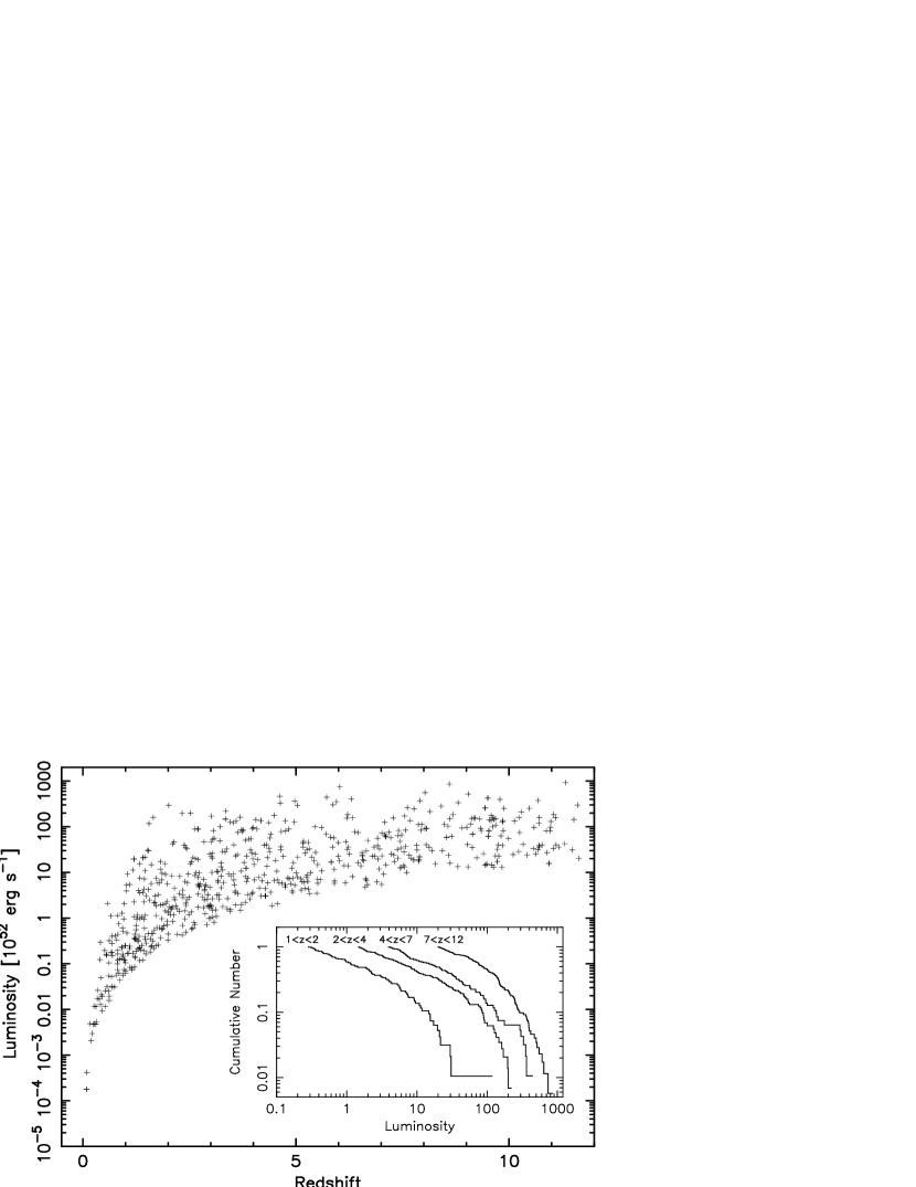
Figure 2: The distribution of luminosity vs. redshift derived from the $E_{p}$–luminosity relation. The truncation of the lower end of the luminosity is caused by the flux limit of $F_{\rm limit}=1\times 10^{-7}~{}{\rm erg~{}cm^{-2}s^{-1}}$. The inserted figure is the cumulative luminosity function in the several redshift ranges. The luminosity evolution exists because the break-luminosity increase toward the higher redshift.

Figure 3: The cumulative luminosity function of $L^{\prime}=L/g_{k}(z)$. This function is equivalent to the present distribution at $z=0$ because the effect of the luminosity evolution $g_{k}(z)$ is removed.

Figure 4: The relative GRB formation rate normalized at the first point. The solid line is the result based on the best fit of $E_{p}$–luminosity relation and two dotted lines indicate the upper and lower bounds caused by the uncertainty of $E_{p}$–luminosity relation. These dotted lines are also normalized and superposed on the best result at $0\leq z\leq 1$ with the least-square method. The error bars accompanying open squares represent the statistical uncertainty of each point.

References

- Amati et al. (2002) Amati, L., Frontera. F., Tavani. M., et al. 2002, A&A, 390, 81
- Andersen et al. (2000) Andersen M. I., Hjorth, J., Pedersen, H., et al. 2000, A&A, 364, L54
- Atteia (2003) Atteia, J-L. 2003, A&A, 407, L1
- Band et al. (1993) Band, D.L., Matteson, J., Ford, L., et al. 1993, ApJ, 413, 281
- Band (2003) Band, D.L., 2003, ApJ, 588, 945
- Barger et al. (2000) Barger, A. J., Cowie, L. L., & Richards, E. A. 2000, AJ, 119, 2092
- Bennett et al. (2003) Bennett, C. L., Halpern, M., Hinshaw, G., et al. astro-ph/0302207
- Bloom et al. (2001) Bloom, J. S., Frail, D. A., & Sari, R. 2001, AJ, 121, 2879
- Bloom et al. (2003) Bloom, J. S., Frail, D. A., & Kulkarni, S. R. 2003, astro-ph/0302210
- Caditz & Petrosian (1990) Caditz, D. & Petrosian, V. 1990, ApJ, 357, 326
- Cowie et al. (1999) Cowie, L. L., Songaila, A., & Barger, A. J. 1999, AJ, 118, 603
- Efron & Petrosian (1992) Efron, B. & Petrosian, V., 1992, ApJ, 399, 345
- Fenimore & Ramirez-Ruiz (2000) Fenimore, E. E., & Ramirez-Ruiz, E. 2000, astro-ph/0004176
- Frail et al. (2001) Frail, D. A., Kulkarni, S. R., Sari, R., et al. 2001, ApJ, 562, L55
- Galama et al. (1998) Galama, T.J., et al. 1998, Nature, 395, 670
- Glazebrook et al. (2003) Glazebrook, K., et al. 2003, ApJ, 587, 55
- Hjorth et al. (2003) Hjorth, J. et al., 2003, Nature, 423, 847
- Ioka & Nakamura (2001) Ioka, K., & Nakamura, T. 2001, ApJL, 554, 163
- Kashikawa et al. (2003) Kashikawa, N., Takata, T., Ohyama, Y., et al. 2003, AJ, 125, 53
- Lanzetta et al. (2003) Lanzetta, K. M., et al. 2003, ApJ, 570, 492
- Lilly et al. (1996) Lilly, S. J., LeFevre, O., Hammer, F., & Crampton, D. 1996, ApJ, 460, L1
- Lloyd et al. (2000) Lloyd, N. M., Petrosian, V., & Mallozzi, R.S. 2000, ApJ, 534, 227
- Lloyd-Ronning et al. (2002) Lloyd-Ronning, N. M., Fryer, C. L. & Ramirez-Ruiz, E. 2002, ApJ, 574, 554
- Lynden-Bell (1971) Lynden-Bell, D. 1971, MNRAS, 155, 95
- Madau et al. (1996) Madau, P., Ferguson, H. C., Dickinson, M. E., et al. 1996, MNRAS, 283, 1388
- Maloney & Petrosian (1999) Maloney, A. & Petrosian, V. 1999, ApJ, 518, 32
- Murakami et al. (2003) Murakami, T., Yonetoku, D., Izawa, H. & Ioka, K. 2003, PASJ,
- Norris et al. (2000) Norris,J., Marani, G.,& Bonnell, J. 2000, ApJ, 534, 248
- Norris (2002) Norris, J. 2000, ApJ, 579, 386
- Petrosian (1993) Petrosian, V. 1993, ApJ, 402, L33
- Price et al. (2000) Price, P.A. et al., 2003, Nature, 423, 844
- Schaefer et al. (2001) Schaefer, B. E., Deng, M. & Band, D. L. 2001 ApJ, 563, L123
- Schaefer (2003a) Schaefer 2003, ApJ, 583, L67
- Schaefer (2003b) Schaefer 2003, ApJ, 583, L71
- Spergel et al. (2003) Spergel, D. N., Verde, L., Peiris, H. V., et al. 2003, astro-ph/0302209
- Stanek et al. (2003) Stanek, K.Z. et al. 2003, ApJ, 591, L71
- Stanway et al. (2003) Stanway, E. R., Bunker, A. J. & McMahon, R. G. 2003, MNRAS, 342, 439
- Uemura et al. (2003) Uemura, M. et al. 2003, Nature, 423, 843
- Yamazaki et al. (2002) Yamazaki, R., Ioka, K. & Nakamura, T. 2002, ApJ, 571, L31
- Yamazaki et al. (2003) Yamazaki, R., Yonetoku, D. & Nakamura, T. 2003, astro-ph/0306615
- Zhang & Mészáros (2002) Zhang, B. & Mészáros, P. 2002, ApJ, 581, 1236