Quantitative Description of the Sunyaev-Zeldovich
Effect: Analytic Approximations

Abstract

Various aspects of relativistic calculations of the Sunyaev-Zeldovich effect are explored and clarified. We first formally show that the main previous approaches to the calculation of the relativistically generalized thermal component of the effect are equivalent. Our detailed description of the full effect results in a somewhat improved formulation. Analytic approximations to the exact calculation of the change of the photon occupation number in the scattering, $\Delta n$, are extended to powers of the gas temperature and cluster velocity that are higher than in similar published treatments. For the purely thermal and purely kinematic components, we obtain identical terms up to the highest common orders in temperature and cluster velocity, and to second order in the Thomson optical depth, as reported in previous treatments, but we get slightly different expressions for the terms that depend on both the gas temperature and cluster velocity. We also obtain an accurate expression for the crossover frequency.

and

1 Introduction

Compton scattering of the cosmic microwave background (CMB) by electrons in the hot gas in clusters of galaxies (Sunyaev & Zeldovich 1972) imprints on the radiation a spectral signature – the Sunyaev-Zeldovich (S-Z) effect – that has long been recognized as a uniquely important feature which can be used as an indispensable cosmological probe. Measurements with single-dish radio telescopes and interferometric arrays have led so far to the detection and imaging of the effect in more than 60 clusters. These measurements yield directly the properties of the hot intracluster (IC) gas, and indirectly the total mass of the cluster, insight on the evolution of clusters, and the values of the basic cosmological parameters (for reviews, see Rephaeli 1995a, Birkinshaw 1999, Carlstrom  et al.  2002).

Exact description of the effect is needed in order to extract precise information from current measurements, and especially from upcoming high-frequency observations. The calculations of Sunyaev & Zeldovich (1972) were based on a solution to the Kompaneets (1957) equation, a nonrelativistic  diffusion approximation to the exact kinetic (Boltzmann) equation that describes the scattering. The result of their treatment is a simple expression for the intensity change resulting from scattering of the CMB by electrons with a thermal velocity distribution. The effect has a second kinematic (Doppler) component which is proportional to the component of the cluster peculiar velocity along the line of sight, $v_{r}$ (Sunyaev & Zeldovich 1980).

Rephaeli (1995b) has shown that the approximate nonrelativistic treatment of Sunyaev & Zeldovich (1972) is not sufficiently accurate for use of the effect as a precise cosmological probe. High electron velocities in the IC gas, and relatively large photon energy change in the scattering, necessitate a more exact relativistic calculation. Using the exact probability distribution, and the relativistically correct form of the electron Maxwellian velocity distribution, Rephaeli calculated the resulting intensity change in the limit of small optical depth to Thomson scattering, $\tau$, keeping terms linear in $\tau$. This semi-analytic calculation demonstrated that the relativistic spectral distribution of the intensity change is appreciably different from that derived by Sunyaev & Zeldovich (1972). Deviations from the Sunyaev & Zeldovich expression are especially large near the crossover frequency, where the purely thermal effect vanishes, and on the Wien side where the effect of boosting photons to relatively high frequencies by energetic electrons is important.

The results of the calculations of Rephaeli (1995b) generated considerable interest that led to various generalizations and extensions of the relativistic treatment. Challinor & Lasenby (1998) obtained an analytic approximation to the solution of the relativistically generalized Kompaneets equation. Nozawa  et al.  (1998a) improved the accuracy of this approximation by expanding to fifth order in $\Theta=kT_{e}/m_{e}c^{2}$, where $T_{e}$ is the electron temperature. Sazonov & Sunyaev (1998) and Nozawa et al. (1998b) have extended the relativistic treatment also to the kinematic component obtaining – for the first time – the leading cross terms in the expression for the combined (thermal and kinematic) intensity change, $\Delta I_{t}+\Delta I_{k}$, which depends on both $T_{e}$ and $v_{c}$, the cluster peculiar velocity. An analytic fit to the numerical solution, valid for $0.02\leq\Theta_{e}\leq 0.05$, and $x\equiv h\nu/kT\leq 20$ (for $\nu\leq 1130$ GHz; $T$ is the CMB temperature), has been given by Nozawa et al. (2000).

Cluster X-ray and S-Z measurements have significantly improved in the last few years. Many nearby and distant clusters have been sensitively mapped spectrally and spatially by the Chandra and XMM satellites, yielding a wealth of information on the complex morphology and thermal structure of IC gas. Interferometric S-Z measurements, and upcoming high resolution observations with bolometric multi-frequency arrays containing large number of elements, expand the scope of S-Z science and further motivate more accurate treatment of the basic effect and its realistic modeling.

In this paper we clarify various aspects of a relativistically exact description of the S-Z effect, and derive accurate analytic expressions for the intensity change and crossover frequency that are valid over wide regions of parameter space. Several different approaches have been adopted in the relativistic calculation of the effect, and although the approximate analytic expressions that were derived in these treatments are either consistent when compared at the same level of accuracy, or yield consistent numerical results, it has not yet been formally shown that the three main approaches to relativistic calculation of the S-Z effect are indeed equivalent. This equivalence is formally proved in Section 2.1. In order to provide more accurate analytic approximation to the thermal component of the effect, we derive – in section 2.2 – an analytic fit to the thermal component of the effect which is accurate to orders $\tau^{1}\Theta^{8}$. In view of the possibility that in some rich clusters $\tau$ is as high as $0.03$, the approximate analytic expansion to first order in $\tau$ and to eighth order in $\Theta$ necessitates also the inclusion of multiple scatterings, of order $\tau^{2}$. This has been considered by Itoh et al. (2001), and is treated further here in section 2.2, where we consider the contribution of two successive scatterings (terms to order $\tau^{2}$) and find that the $\tau^{2}\Theta^{2}$ – $\tau^{2}\Theta^{5}$ contributions are appreciable near the crossover frequency for which we derive an analytic approximation. In section 2.2 we also include an analytic expression for the change in the photon occupation number that is accurate for gas temperatures as high as 50 keV. In sections 2.3 and 2.4 the kinematic and the full effect are calculated, including the cross terms that depend on both the gas temperature and the cluster velocity. Our results for these terms differ somewhat from those obtained by other groups. The last section (3) contains a more general discussion of the results presented in this paper.

2 Exact Description of the S-Z Effect

In this section we explicitly calculate the thermal, kinematic and cross terms of the S-Z effect. While such calculations have already been carried out in various papers, our approach here is more direct, and the results are roughly at the same level of accuracy as achieved in the recent work of Itoh & Nozawa (2003), where the results of a numerical fit are given in a tabulated form. Following a detailed description of the full effect, and our analytic approximations, we present a fit to the exact calculation that is valid at gas temperature well beyond 15 keV. We begin with a general comparison of the main theoretical descriptions of the effect.

2.1 Equivalent Relativistic Treatments

Three main approaches have been adopted in the calculation of the relativistic S-Z effect, those employed by Rephaeli (1995a), Sazonov & Sunyaev (1998), and Nozawa et al. (1998a). Different analytic approximations to the exact expressions that were obtained in these treatments were found to be consistent when compared to the highest common order of $\Theta$. Here we formally prove that these three approaches are indeed equivalent. Basically, this follows from the fact that although the method used by Nozawa et al. (1998a) is more general than those used by Rephaeli (1995a, 1995b) and Sazonov & Sunyaev (1998), the simplifying assumptions made in deriving analytic approximations, namely neglecting electron recoil, and expansion in powers of a small quantity – the ratio of the change in the photon energy to the photon energy – render it equivalent to the other two approaches.

Consider first the method employed by Rephaeli (1995a, 1995b). The probability of scattering of an incoming photon (direction $\mu_{0}=\cos\theta_{0}$) to the direction $\mu^{\prime}_{0}=\cos\theta^{\prime}_{0}$ is (Chandrasekhar 1950)

$$f\left(\mu_{0},\mu^{\prime}_{0}\right)=\frac{3}{8}\left[1+\mu_{0}^{2}\mu^{\prime 2}_{0}+\frac{1}{2}\left(1-\mu_{0}^{2}\right)\left(1-\mu^{\prime 2}_{0}\right)\right]$$ (1)

where the subscript 0 refers to the electron rest frame. The frequency shift is

$$s=\ln\left(\nu^{\prime}/\nu\right)=\ln\left(\frac{1+\beta\mu^{\prime}_{0}}{1+\beta\mu_{0}}\right)$$ (2)

where $\nu$, $\nu^{\prime}$ are the frequency of the photon before and after the scattering, and $\beta=v/c$ is the dimensionless electron velocity in the CMB frame. It is somewhat more convenient to use the variables $\mu,s$ and $\beta$ instead of $\mu,\mu^{\prime}$ and $\beta$. The probability that a scattering results in a frequency shift $s$ is (Wright 1979)

$$\mathcal{P}\left(s,\beta\right)=\frac{1}{2\gamma^{4}\beta}\int\frac{e^{s}f\left(\mu_{0},\mu^{\prime}_{0}\right)}{\left(1+\beta\mu_{0}\right)^{2}}d\mu_{0}.$$ (3)

Averaging over a Maxwellian distribution for the electrons yields

$$\mathcal{P}_{1}\left(s\right)=\frac{\int\beta^{2}\gamma^{5}e^{-\frac{\left(\gamma-1\right)}{\Theta}}\mathcal{P}\left(s,\beta\right)d\beta}{\int\beta^{2}\gamma^{5}e^{-\frac{\left(\gamma-1\right)}{\Theta}}d\beta}.$$ (4)

The total change in the photon occupation number along a line of sight (los) to the cluster, due to scattering off electrons with thermal ($t$) velocities, can now be written as

$$\Delta n_{t}(x)=\tau\int_{-\infty}^{\infty}\left[n\left(xe^{s}\right)-n\left(x\right)\right]\mathcal{P}_{1}\left(s\right)ds$$ (5)

where $x$ is the dimensionless frequency, $x=h\nu/kT$, and $\tau\equiv\sigma_{T}\int n_{e}dl$ is the optical depth to Thomson scattering.

In the approach of Sazonov & Sunyaev (1998), which is similar to that of Rephaeli (1995a), the starting point is the photon transfer equation

$$\frac{dn_{0}}{dt_{0}}(\mu_{0},\nu_{0})=cn_{e0}\int\frac{d\sigma}{d\Omega^{\prime}_{0}}\left[n_{0}\left(\mu^{\prime}_{0},\nu_{0}\right)-n_{0}\left(\mu_{0},\nu_{0}\right)\right]d\Omega^{\prime}_{0},$$ (6)

where the Planckian occupation number is

$$n_{0}=\frac{1}{e^{x_{0}\gamma\left(1+\beta\mu_{0}\right)}-1},$$ (7)

and $n_{e0}$ & $\mu_{0}$ are the electron number density and the cosine of the angle between the directions of the electron motion, and the photon velocity as seen in this frame, respectively. The differential scattering cross section in the electron rest frame is

$$\frac{d\sigma}{d\Omega^{\prime}_{0}}=\frac{1}{2}\sigma_{T}f(\mu_{0},\mu^{\prime}_{0}),$$ (8)

where $\sigma_{T}$ is the Thomson cross section. Lorentz transformation of equation (6) with $n_{e0}=n_{e}/\gamma$ leads to

$$\frac{dn_{0}}{dt}(\mu_{0},\nu_{0})=\int\frac{cn_{e}}{\gamma^{2}\left(1+\beta\mu_{0}\right)}\delta n\frac{d\sigma}{d\Omega^{\prime}_{0}}d\Omega^{\prime}_{0},$$ (9)

where

$$\delta n\equiv n_{0}\left(\mu^{\prime}_{0},\nu_{0}\right)-n_{0}\left(\mu_{0},\nu_{0}\right)=\frac{1}{e^{xz}-1}-\frac{1}{e^{x}-1}.$$ (10)

Now, in the Thomson limit,

$$z = \frac{1+\beta\mu^{\prime}_{0}}{1+\beta\mu_{0}},$$ (11)

and

$$\frac{dn_{t}}{d\tau}=\int\int\int\frac{d\sigma}{d\Omega^{\prime}_{0}}\frac{\delta n}{\left(1+\beta\mu_{0}\right)^{3}}e^{-\frac{\gamma-1}{\Theta}}d\mu_{0}d\mu^{\prime}_{0}\gamma\beta^{2}d\beta/D$$ (12)

where

$$D=\int_{0}^{1}e^{-\frac{\gamma-1}{\Theta}}\gamma^{5}\beta^{2}d\beta.$$ (13)

This is exactly the expression that was derived by Rephaeli (1995a, 1995b) using a different approach, hence the two methods are shown to be fully equivalent.

In the third method, that of Nozawa et al. (1998a), the starting point is a more basic expression for the time rate of change of the photon occupation number given by a generalized Kompaneets equation

$$\frac{\partial n}{\partial t}\left(\omega\right) = -2\int\int\int\frac{d^{3}p}{\left(2\pi\right)^{3}}d^{3}p^{\prime}d^{3}k^{\prime}W\left[n\left(\omega\right)\left(1+n\left(\omega^{\prime}\right)\right)P_{e}\left(E\right)\right.$$ (14)

$$- \left.n\left(\omega^{\prime}\right)\left(1+n\left(\omega\right)\right)P_{e}\left(E^{\prime}\right)\right],$$

where

$$W \equiv \left(\frac{e^{2}}{4\pi}\right)^{2}\frac{X}{2\omega\omega^{\prime}EE^{\prime}}\delta^{4}\left(p+k-p^{\prime}-k^{\prime}\right),$$ (15)

$$X \equiv -\left(\frac{\rho}{\rho^{\prime}}+\frac{\rho^{\prime}}{\rho}\right)+4m^{4}\left(\frac{\rho}{\rho^{\prime}}+\frac{\rho^{\prime}}{\rho}\right)^{2}-4m^{2}\left(\frac{1}{\rho}+\frac{1}{\rho^{\prime}}\right),$$ (16)

$$\rho \equiv -2\left(p\cdot k\right)=-2\omega E\left(1-\beta\mu_{0}\right),$$ (17)

$$\rho^{\prime} \equiv 2\left(p\cdot k^{\prime}\right)=2\omega^{\prime}E\left(1-\beta\mu^{\prime}_{0}\right),$$ (18)

$p$ and $k$ ($p^{\prime}$ and $k^{\prime}$) are the ingoing (outgoing) electron and photon 4-momentum ($p=(E,\vec{p})$, $k=(\omega,\vec{k})$, $p^{\prime}=(E^{\prime},\vec{p^{\prime}})$, $k^{\prime}=(\omega^{\prime},\vec{k^{\prime}})$), and $\mu_{0}$ ($\mu^{\prime}_{0}$) is the cosine angle between $\vec{k}$ and $\vec{p}$ ($\vec{k^{\prime}}$ and $\vec{p^{\prime}}$) in the electron rest frame. $m$ and $e$ are the electron mass and electric charge and $P_{e}(E)$ is the electron energy distribution.

In the Thomson limit, $\omega^{\prime}_{0}=\omega_{0}$, therefore $E=E^{\prime}$, and Equation (14) simplifies to

$$\frac{\partial n}{\partial t}\left(x\right) = -2\int\frac{d^{3}p}{\left(2\pi\right)^{3}}d^{3}k^{\prime}W\left[n\left(x\right)-n\left(x^{\prime}\right)\right]P_{e}\left(E\right).$$ (19)

Now $X$ is essentially the differential cross section, equation (8), used by Rephaeli (1995a) and Sazonov & Sunyaev (1998) in a less general form. The approximations made by Nozawa et al. (1998a) are based on the fact that $\Delta x\ll 1$ in the CMB frame (which is in fact, used as a perturbation parameter), and that $T/T_{e}\ll 1$. However, since $h\nu/(m_{e}c^{2}\Theta)=h\nu/kT_{e}\sim T/T_{e}\ll 1$, it follows that $h\nu/m_{e}c^{2}\ll\Theta$, and the Thomson limit is valid. Note that $\Delta x\ll 1$ implies that $\beta\ll 1$, and therefore the condition $h\nu/(m_{e}c^{2})\ll 1$ still holds in the electron rest frame. It can now be seen that even though the treatment of Nozawa et al. (1998a) is seemingly more general, their final expression – in the limit when the commonly adopted approximations are valid – reduces to those obtained by Rephaeli (1995a) and Sazonov & Sunyaev (1998). Therefore, all the three methods are equivalent and will therefore yield equivalent results to all orders in $\Theta$, provided the expansion in $\Theta$ is valid ($\Theta\ll 1$).

2.2 The Thermal Component

2.2.1 Single Scattering Limit

In an optically very thin medium with $\tau\leq 0.01$, only single scatterings of CMB photons need to be (practically) considered, and the leading term in the expression for $\Delta n$ is (by far) of order $\tau$. Using equation (9) with an integral over (relativistically generalized expression for) a Maxwellian distribution of electron velocities, we obtain

$$\frac{dn_{t}}{dt} = \frac{1}{D}\int_{\beta=0}^{1}\int_{\mu^{\prime}_{0}=-1}^{1}\int_{\mu_{0}=-1}^{1}\frac{cn_{e}}{\gamma^{4}\left(1+\beta\mu_{0}\right)^{3}}\frac{d\sigma}{d\Omega^{\prime}_{0}}\delta ne^{-\frac{\gamma-1}{\Theta}}\gamma^{5}\beta^{2}d\beta d\mu^{\prime}_{0}d\mu_{0}.$$ (20)

To first order in $\tau$, $\Delta n$ is

$$\Delta n_{t} = \frac{\tau}{2D}\int_{\beta=0}^{1}\int_{\mu^{\prime}_{0}=-1}^{1}\int_{\mu_{0}=-1}^{1}\frac{\delta n}{\gamma^{4}\left(1+\beta\mu_{0}\right)^{3}}f\left(\mu_{0},\mu^{\prime}_{0}\right)e^{-\frac{\gamma-1}{\Theta}}\gamma^{5}\beta^{2}d\beta d\mu^{\prime}_{0}d\mu_{0}.$$ (21)

To perform the integrations in this expression, we expand the integrand in powers of $\beta$ around $\beta=0$ with the derivatives (at $\beta=0$) compactly written by defining

$$A_{n}=-2^{n-2}x^{n}[\sinh^{-2}\frac{x}{2}]^{(n-1)},$$ (22)

where $f^{(n)}$ denotes the n’th derivative of $f$. Carrying out the expansion to $\beta^{16}$ and integrating yield

$$\frac{\Delta n_{t}}{\tau} = \Theta F_{1}+\Theta^{2}F_{2}+\Theta^{3}F_{3}+\Theta^{4}F_{4}+\Theta^{5}F_{5}+\Theta^{6}F_{6}+\Theta^{7}F_{7}+\Theta^{8}F_{8}$$ (23)

where $F_{i}$ are listed in Appendix A.

It is instructive to compare our result in equation (23) to equations (2.25)-(2.30) of Nozawa et al. (1998a) that were obtained using a different approach. The functions $A_{i}$ can be expressed in terms of $\tilde{X}$ and $\tilde{S}$

$$\tilde{X} \equiv x\coth\frac{x}{2},$$

$$\tilde{S} \equiv \frac{x}{\sinh\frac{x}{2}},$$ (24)

and the relations between $A_{i}$, $\tilde{X}$ and $\tilde{S}$ are given in Appendix B. Substituting the expressions in Appendix B back into $F_{1}$ - $F_{5}$ and equation (24), we obtain exactly equations (2.25)-(2.30) of Nozawa et al. (1998a) term by term. This is, of course, just what we expect given the proven equivalence of the approaches discussed above.

2.2.2 Multiple Scatterings

Although formally very accurate, the single scattering analytic approximation to order $\Theta^{8}$ is actually limited to small values of $\tau$. This optical depth is typically $\sim 0.01$ in a rich cluster, but values as high as of up to $0.03$ are not unexpected in some clusters. Thus, the possibility of double scatterings is not ignorable to the level of accuracy afforded by the above expansion to order $\tau\Theta^{8}$. A more self consistent calculation must include the higher order terms up to $\tau^{2}\Theta^{5}$, which can be comparable to the $\tau\Theta^{8}$ term. The importance of considering the case of finite optical depth was already pointed out by Molnar & Birkinshaw (1999), Itoh et al. (2001), and Dolgov et al. (2001). Our goal here is to extend the analytic approximation by calculating all the relevant contributions up to and including terms that are of order $\tau^{2}\Theta^{5}$.

The impact of second scatterings on the occupation number can be calculated iteratively by describing the incident radiation in terms of the occupation number, $n_{1}$, that results after the radiation has already been singly scattered. In this way one can extend the treatment to the case of any number of scatterings (Wright 1979). Now, $n_{1}$ is simply

$$n_{1}=n_{0}+\Delta n_{0},$$ (25)

where $\Delta n_{0}$ is given in equation (23). Substituting $n_{1}$ into the right hand side of equation (12) we can solve for $\Delta n_{1}$. Note that the result of the naive iteration should be divided by $2!$ to avoid double counting; a given total frequency shift ($\nu^{\prime}/\nu=z$) results from two scatterings irrespective of the order of the two scattering events. The expression for the occupation number of the doubly scattered radiation is

$$n^{\prime}=e^{-\tau}\left(n_{0}+\tau n_{0}\otimes\mathcal{P}+\frac{1}{2}\tau^{2}n_{0}\otimes\mathcal{P}\otimes\mathcal{P}\right),$$ (26)

where $\otimes$ denotes convolution and (as before) $\mathcal{P}$ is the scattering probability, equation (3). Expanding the exponent to second order in $\tau$, we have

$$\Delta n_{t} = \left(\tau-\frac{1}{2}\tau^{2}\right)\left(n\otimes\mathcal{P}-n\right)+\frac{1}{2}\tau^{2}\left(n\otimes\mathcal{P}\otimes\mathcal{P}-n\otimes\mathcal{P}\right).$$ (27)

The first term on the right hand side of equation (27) ($n\otimes\mathcal{P}-n$) was evaluated in section 2.2.1; here we calculate the $\tau^{2}$ contribution. Performing the integrations in a way similar to the calculation of the first order $\tau$ contribution, we obtain

$$\frac{1}{2}\tau^{2}(n\otimes\mathcal{P}\otimes\mathcal{P}-n\otimes\mathcal{P})=\tau^{2}\Theta^{2}F_{9}+\tau^{2}\Theta^{3}F_{10}+\tau^{2}\Theta^{4}F_{11}$$ (28)

$$+ \tau^{2}\Theta^{5}F_{12}.$$

Altogether, the resulting change in the occupation number calculated to orders $\tau\Theta^{8}$ and $\tau^{2}\Theta^{5}$ is

$$\Delta n_{t} = \tau(\Theta F_{1}+\Theta^{2}F_{2}+\Theta^{3}F_{3}+\Theta^{4}F_{4}+\Theta^{5}F_{5}+\Theta^{6}F_{6}+\Theta^{7}F_{7}$$ (29)

$$+ \Theta^{8}F_{8})+\tau^{2}(\Theta^{2}F_{9}+\Theta^{3}F_{10}+\Theta^{4}F_{11}+\Theta^{5}F_{12}).$$

It can be easily shown that equation (29) satisfies photon number conservation.

The $\tau^{2}$ terms are important especially near the crossover frequency, whose value depends both on $\Theta$ and $\tau$, as derived explicitly below. Also of interest is the unignorable effect of double scatterings at frequencies on the far Wien side of the spectrum, due to the fact that the total change in the frequency of the photon after two scatterings is particularly high. More specifically, we examined the contribution of these terms to $\Delta I$. For $\tau$ in the range [0.01,0.04] and $\Theta$ in the range [1/130, 1/35], the corrections due to these terms are larger than $1\%$ near the crossover frequency as expected. Clearly, the spectral band around this frequency – for which the corrections are not ignorable – widens as $\Theta$ increases.

2.2.3 Analytic Fit to the Thermal Effect

The observed range of IC gas temperatures is $\sim 3-15$ keV, when the gas is taken to be isothermal (in the fit to the observed X-ray spectrum). High spatial and spectral resolution measurements with the Chandra and XMM satellites show more and more that the temperature distribution is non-uniform, which is only to be expected given the hierarchical growth of structure in the context of CDM models. A more realistic modeling of IC gas yields hotter and colder regions in some clusters, perhaps reflecting the nature of the formation process of clusters from aggregates or sub-clumps. In a naive modeling of the temperature evolution of clusters a virial mass-temperature relation is sometimes obtained with clusters of a given mass having a higher temperature the earlier they virialized. If so, a roughly linear relation would be predicted between the temperature and the virialization redshift of the cluster. Irrespective of the reality of such a scaling, it is of interest to extend the accuracy of the analytic approximations for $\Delta n$ to values of $kT_{e}$ which are higher than $15$ keV. Equation (23) is not sufficiently accurate at higher temperatures because the series expansion does not converge and rapidly oscillates around the exact numerical result (equation 21).

Here we obtain a more accurate fit to the results from the exact calculation using a polynomial function of the form

$$\Delta n(x)/\tau=\sum_{i=1}^{5}\sum_{j=1}^{10}b_{ij}A_{j}\Theta^{i}=\sum_{i=1}^{5}H_{i}\Theta^{i}$$ (30)

where the numerical coefficients $b_{ij}$ are obtained by means of a best fit to the exact expression (equation 21). The coefficients $H_{i}$ are given in Appendix A. This expression is in agreement with the exact calculation to better than 2.5% for $\Theta<1/10$, or $kT_{e}<50$ keV. This level of accuracy is higher than that obtained by Itoh et al. (2001) who used the analytic expansion (equation 23). Evidently, higher accuracy is attained by not insisting on using the exact form of the analytic expansion also at higher temperatures; our approach is thus functionally less constrained. Very recently, Itoh & Nozawa (2003) have extended their previous analytic approximation for $\Delta n$ to higher temperatures by fitting the results of the exact numerical calculation with a polynomial of order $\Theta^{5}$ for $x<1.2$, and a fully numerical fit to a polynomial in powers of both $\Theta$ (to 13th order) and $x$ for $x>1.2$ (with the large array of coefficients given in a tabulated form). This more cumbersome procedure does result in a more accurate representation of the exact numerical calculation, which is generally within $0.4\%$.

2.2.4 Crossover Frequency

As was pointed out in Rephaeli (1995b), Sazonov & Sunyaev (1998) and Nozawa et al. (1998a), the crossover frequency ($x_{0}$) depends on the gas temperature. In previously derived expressions for the functional form of $x_{0}$, only the dependence on $\Theta$ was considered, and deduced from a $\chi^{2}$ fit. In order to find an analytic approximation to the shifted crossover frequency we write

$$x_{0} = 3.8300161\left(1+c_{1}\Theta+c_{2}\Theta^{2}+c_{3}\Theta^{3}+c_{4}\Theta^{4}+c_{5}\tau+c_{6}\tau\Theta\right.$$ (31)

$$+ \left.c_{7}\tau\Theta^{2}\right),$$

and substitute this expression in equation (29). Expanding in the small parameters $\tau$ and $\Theta$, we then obtain the values of the coefficients in the expression for $x_{0}$ by setting $\Delta n_{t}=0$,

$$x_{0} = 3.830016\left(1+1.120594\Theta+2.078258\Theta^{2}-80.748072\Theta^{3}\right.$$

$$+ \left.1548.250996\Theta^{4}+0.800424\tau\Theta+1.183073\tau\Theta^{2}\right).$$

It can be readily shown that, as expected, $x_{0}$ monotonically increases with $\tau$ and $\Theta$.

2.3 The Kinematic Component

In an idealized cold IC gas all electrons have the same velocity in the CMB frame – the cluster peculiar velocity, $\beta_{c}$. Substituting $\beta_{c}$ for $\beta$ in equation (9), and applying the Lorentz transformation

$$\mu_{0}=\frac{\mu_{c}-\beta_{c}}{1-\beta_{c}\mu_{c}}$$ (32)

where $\mu_{c}$ is the angle cosine with respect to the los of an observer (as measured in the CMB frame), we obtain

$$\Delta n = \frac{3}{32}\tau\left(1-\beta_{c}\mu_{c}\right)$$ (33)

$$\times \int\left[\left(3-\mu^{\prime 2}_{0}\right)+\left(3\mu^{\prime 2}_{0}-1\right)\left(\frac{\mu_{c}-\beta_{c}}{1-\beta_{c}\mu_{c}}\right)^{2}\right]\delta nd\mu^{\prime}_{0},$$

where $\delta n$ is given in eq. (10), and

$$z=\frac{1+\beta\mu^{\prime}_{0}}{1+\beta\mu_{0}}=\gamma_{c}^{2}\left(1+\beta_{c}\mu^{\prime}_{0}\right)\left(1-\beta_{c}\mu_{c}\right).$$ (34)

We evaluate the latter expression for $\Delta n$ as part of the calculation of the full effect in the next section.

2.4 The Full Effect

To first approximation, when $\Theta$ and $\beta_{c}$ are sufficiently small, the impact on the CMB by Compton scattering in a cluster with finite peculiar velocity is simply a sum of the thermal and kinematic components. For higher values of $\Theta$ and $\beta_{c}$, higher order terms have to be included. As a result, cross terms linking the two components arise. The inclusion of the peculiar velocity of the cluster in a consistent calculation (not as a separate effect) was originally considered by Sazonov & Sunyaev (1998), and later also by Nozawa et al. (1998b). Their calculations yield consistent results for the cross terms that depend on both $\Theta$ and $\beta_{c}$. We repeat the calculation of the full effect by generalizing our treatment described in the previous sections. We do so in part because our calculation yields slightly different results for the cross terms, although our results for the pure thermal and kinematic components are exactly identical to those obtained in the latter papers.

We begin with the transformation of the electron thermal energy and momentum, $E_{t}$ and $\vec{p}_{t}$, from the cluster to the CMB frame, $E$ and $\vec{p}$, respectively

$$E = \gamma_{c}\left(E_{t}+c\vec{\beta}_{c}\cdot\vec{p}_{t}\right)$$

$$\vec{p} = \gamma_{c}\left(\vec{p}_{t}+\vec{\beta}_{c}E_{t}/c\right).$$ (35)

Applying these transformations in the expression for the Boltzmann factor we obtain

$$\exp\left(-\frac{E_{t}-m_{e}c^{2}}{kT_{e}}\right)=\exp\left(-\frac{\gamma_{t}-1}{\Theta}\right)$$

$$=\exp\left(-\frac{\gamma_{c}\gamma(1-\vec{\beta}\cdot\vec{\beta}_{c})-1}{\Theta}\right),$$ (36)

where $\beta$ and $\gamma$ are the velocity and Lorentz factor in the CMB frame.

Since $d^{3}p/E$ is invariant under Lorentz transformations,

$$d^{3}p_{t} = \frac{E_{t}}{E}d^{3}p=\gamma_{c}\left(1-\vec{\beta}_{c}\cdot\vec{\beta}\right)p^{2}dpd\mu d\varphi$$ (37)

$$= \gamma_{c}\left(1-\vec{\beta}_{c}\cdot\vec{\beta}\right)\gamma^{5}\beta^{2}d\beta d\mu d\varphi.$$

Expanding to second order in $\beta_{c}$ we obtain

$$p_{t}^{2}dp_{t}\exp\left(-\frac{\gamma_{t}-1}{\Theta}\right)=$$ (38)

$$= \gamma_{c}\left(1-\vec{\beta}_{c}\cdot\vec{\beta}_{t}\right)\exp\left(-\frac{\gamma_{c}\gamma\left(1-\vec{\beta}\cdot\vec{\beta}_{c}\right)-1}{\Theta}\right)\gamma^{5}\beta^{2}d\beta\approx$$

$$\approx \left[1+\vec{\beta}_{c}\cdot\vec{\beta}\left(\frac{\gamma}{\Theta}-1\right)+\left[\frac{\beta_{c}^{2}}{2}\left(1-\frac{\gamma}{\Theta}\right)+\left(\vec{\beta}_{c}\cdot\vec{\beta}\right)^{2}\left(\frac{\gamma^{2}}{2\Theta^{2}}-\frac{\gamma}{\Theta}\right)\right]\right]$$

$$\times \exp\left(-\frac{\gamma-1}{\Theta}\right)\gamma^{5}\beta^{2}d\beta.$$

Note that

$$\vec{\beta}_{c}\cdot\vec{\beta} = \beta_{c}\beta\left(\cos\theta\cos\theta_{c}+\cos\varphi\sin\theta\sin\theta_{c}\right)$$

$$\cos\theta = \frac{\cos\theta_{0}+\beta}{1+\beta\cos\theta_{0}}$$ (39)

where $\theta$ and $\theta_{c}$ are angles in the cosmic frame and $\theta_{0}$ is in the electron rest frame; we select axes such that $\varphi_{c}=0$). Integrating over the azimuthal angle $\varphi$ (divided by $2\pi$) and expanding again near $\beta_{c}=0$, we obtain

$$p_{t}^{2}dp_{t}\exp\left(-\frac{\gamma_{t}-1}{\Theta}\right)\approx$$ (40)

$$\left[1+\beta_{c}\beta\mu_{c}\mu\left(\frac{\gamma}{\Theta}-1\right)+\frac{1}{2}\beta_{c}^{2}\beta^{2}\left(\mu_{c}^{2}-\frac{1}{3}\right)\left(3\mu^{2}-1\right)\left(\frac{1}{2}\frac{\gamma^{2}}{\Theta^{2}}-\frac{\gamma}{\Theta}\right)\right.$$

$$+ \left.\beta_{c}^{2}\left(\frac{\beta^{2}\gamma^{2}}{6\Theta^{2}}-\frac{\beta^{2}\gamma}{3\Theta}+\frac{1}{2}-\frac{\gamma}{2\Theta}\right)\right]\exp\left(-\frac{\gamma-1}{\Theta}\right)\gamma^{5}\beta^{2}d\beta.$$

Substituting this into the transfer equation (Equation (21)) and performing the integrations yield the correction to the thermal effect, Equation (23)

$$\Delta n/\tau = -\beta_{c}\mu_{c}\left(\frac{1}{2}A_{1}+\Theta F_{13}+\Theta^{2}F_{14}+\Theta^{3}F_{15}+\Theta^{4}F_{16}\right)$$ (41)

$$+ \beta_{c}^{2}P_{2}\left(\mu_{c}\right)\left(F_{17}+\Theta F_{18}+\Theta^{2}F_{19}+\Theta^{3}F_{20}+\Theta^{4}F_{21}\right)$$

$$+ \beta_{c}^{2}\left(\frac{1}{3}F_{1}+\Theta F_{22}+\Theta^{2}F_{23}+\Theta^{3}F_{24}+\Theta^{4}F_{25}\right),$$

where $F_{i}$ are found in Appendix A.

The purely kinematic terms in equation (41) are identical to the corresponding terms in similar equations obtained by Sazonov & Sunyaev (1998) and Nozawa et al. (1998b). However, our results for the cross terms differ somewhat from those obtained in the latter two papers. The difference is due to integration of the transfer equation over $\gamma^{5}\beta^{2}d\beta d\mu d\varphi$, rather than over equation (37) – as we have done here – which includes the extra factor $\gamma_{c}(1-\vec{\beta}_{c}\cdot\vec{\beta})$. From a practical point of view this difference is quite small, typically less than 1%. We note that both our result, equation (41), and the results derived in all the latter three papers satisfy photon number conservation.

3 Discussion

In this paper we have first shown that the three main, seemingly different approaches to the calculation of relativistic corrections to the expressions of Sunyaev & Zeldovich (1972), are indeed equivalent in the limiting case for which they are derived. We then extended the accuracy of the analytic approximation to the thermal and kinematic terms such that the purely thermal component of the effect is accurate to terms of order $\Theta^{8}$, and the cross terms to order $\beta_{c}^{2}\Theta^{4}$. We have also obtained a relatively compact fit to the exact numerical calculation of $\Delta n$ that is accurate to within 2.5% for gas temperatures as high as 50 keV. Either this functional fit, or the more accurate – but perhaps somewhat less convenient – fully numerical tabulation of Itoh & Nozawa (2003), can be used in the analysis of SZ measurements – including cosmological parameter determination – whose current observational errors are well above the accuracies provided by these fits.

While the accuracy of these expressions is limited very close to the crossover frequency, this is usually of little practical consequence because of the typically broad detector spectral response: Even when the measurements are made very close to the crossover frequency for the purpose of measuring cluster peculiar velocities, what is required is only a sufficiently accurate value of the $\Delta I$ convolved over the spectral response. The analytic expression given here is accurate to within a few %. Convolving both the exact (eq. 21) and the approximate expressions (eqs. 23 & 30) over a Gaussian detector response centered at 214 GHz, and with a FWHM of 30 GHz (characteristics of the second MITO channel), we find that the two results agree to within 0.2%. Thus, the impact of this small difference (close to the crossover frequency) on the determination of cluster peculiar velocities is expected to be negligible.

The accuracy of the theoretical description of the SZ effect surpasses the precision with which the effect can be measured at present. In addition to observational errors, systematic modeling uncertainties are relatively large. One of these uncertainties stems from the unknown gas temperature profile. From a theoretical point of view this can be readily assessed for a given assumed profile. For example, consider the case of an idealized (and perhaps somewhat unrealistic) polytropic equation of state $P\propto\rho^{\gamma}$, where $\gamma$ is a free parameter which is determined from X-ray measurements. In order to generalize our result for the analytic approximation for $\Delta n$ to the case of non-isothermal gas, we need to replace the spatially dependent parameters by their appropriately weighted expressions. Consider, for example, the commonly used $\beta$ model for the gas density, $n_{e}(r)\propto[1+(r/r_{c})^{2}]^{-3\beta/2}$, where $r_{c}$ is the gas core radius. (Note that here $\gamma$ and $\beta$ denote different quantities than those in the rest of the paper.) Since $T_{e}\propto\rho^{1-\gamma}$, the products of $\tau\Theta^{i}$ that appear in the analytic approximation for $\Delta n$ have to be replaced by weighted averages along the los

$$\bar{\tau\Theta^{i}}=\tau_{0}\Theta_{0}^{i}\int_{-z}^{z}(1+x^{2})^{-\frac{3}{2}\beta\left[1+\left(\gamma-1\right)i\right]}dx$$ (42)

where $z$ is the radial extent of the gas distribution in units of the core radius, $n_{0}$ & $T_{0}$ are the central values of the electron density and temperature, and $\tau_{0}=2\sigma_{T}n_{0}r_{c}$.

Appendix A

The following is a list of the functions $F_{i}$, $G_{i}$ and $H_{i}$ in terms of the functions $A_{j}$ [defined in Equation (22)]

$$F_{1} = 2A_{1}+\frac{1}{4}A_{2}$$

$$F_{2} = 5A_{1}+\frac{47}{8}A_{2}+\frac{21}{20}A_{3}+\frac{7}{160}A_{4}$$

$$F_{3} = \frac{15}{4}A_{1}+\frac{1023}{32}A_{2}+\frac{217}{10}A_{3}+\frac{329}{80}A_{4}+\frac{11}{40}A_{5}+\frac{11}{1920}A_{6}$$

$$F_{4} = -\frac{15}{4}A_{1}+\frac{2505}{32}A_{2}+\frac{3549}{20}A_{3}+\frac{14253}{160}A_{4}+\frac{9297}{560}A_{5}$$

$$+ \frac{12059}{8960}A_{6}+\frac{1}{21}A_{7}+\frac{1}{1680}A_{8}$$

$$F_{5} = \frac{135}{64}A_{1}+\frac{30375}{512}A_{2}+\frac{62391}{80}A_{3}+\frac{614727}{640}A_{4}+\frac{124389}{320}A_{5}$$

$$+ \frac{355703}{5120}A_{6}+\frac{2071}{336}A_{7}+\frac{1879}{6720}A_{8}+\frac{11}{1792}A_{9}+\frac{11}{215040}A_{10}$$

$$F_{6} = \frac{45}{16}A_{1}-\frac{7515}{128}A_{2}+\frac{28917}{16}A_{3}+\frac{795429}{128}A_{4}+\frac{2319993}{448}A_{5}$$

$$+ \frac{12667283}{7168}A_{6}+\frac{201631}{672}A_{7}+\frac{10655}{384}A_{8}+\frac{46679}{32256}A_{9}+\frac{10853}{258048}A_{10}$$

$$+ \frac{29}{46080}A_{11}+\frac{29}{7741440}A_{12}$$

$$F_{7} = -\frac{7425}{512}A_{1}+\frac{128655}{4096}A_{2}+\frac{360675}{256}A_{3}+\frac{50853555}{2048}A_{4}+\frac{45719721}{1024}A_{5}$$

$$+ \frac{458203107}{16384}A_{6}+\frac{22251961}{2688}A_{7}+\frac{71548297}{53760}A_{8}+\frac{26865067}{215040}A_{9}$$

$$+ \frac{7313155}{1032192}A_{10}+\frac{1123}{4608}A_{11}+\frac{6361}{1290240}A_{12}+\frac{37}{691200}A_{13}+\frac{37}{154828800}A_{14}$$

$$F_{8} = \frac{675}{16}A_{1}+\frac{6345}{128}A_{2}-\frac{86751}{64}A_{3}+\frac{28579473}{512}A_{4}+\frac{463090581}{1792}A_{5}$$

$$+ \frac{8680356807}{28672}A_{6}+\frac{407333911}{2688}A_{7}+\frac{304758409}{7680}A_{8}+\frac{14281971623}{2365440}A_{9}$$

$$+ \frac{32154229291}{56770560}A_{10}+\frac{17138321}{506880}A_{11}+\frac{36841447}{28385280}A_{12}+\frac{481771}{15206400}A_{13}$$

$$+ \frac{229693}{486604800}A_{14}+\frac{23}{5913600}A_{15}+\frac{23}{1703116800}A_{16}$$

$$F_{9} = 4A_{1}+\frac{17}{4}A_{2}+\frac{3}{4}A_{3}+\frac{1}{32}A_{4}$$

$$F_{10} = 20A_{1}+\frac{295}{4}A_{2}+\frac{873}{20}A_{3}+\frac{1271}{160}A_{4}+\frac{21}{40}A_{5}+\frac{7}{640}A_{6}$$

$$F_{11} = 40A_{1}+599A_{2}+\frac{44643}{50}A_{3}+\frac{19557}{50}A_{4}+\frac{27549}{400}A_{5}+\frac{34873}{6400}A_{6}$$

$$+ \frac{367}{1920}A_{7}+\frac{367}{153600}A_{8}$$

$$F_{12} = \frac{45}{2}A_{1}+\frac{96651}{32}A_{2}+\frac{8659449}{800}A_{3}+\frac{62384943}{6400}A_{4}+\frac{38586081}{11200}A_{5}$$

$$+ \frac{103117227}{179200}A_{6}+\frac{82813}{1680}A_{7}+\frac{590831}{268800}A_{8}+\frac{859}{17920}A_{9}+\frac{859}{2150400}A_{10}$$

$$F_{13} = \frac{9}{2}A_{1}+\frac{47}{20}A_{2}+\frac{7}{40}A_{3}$$

$$F_{14} = \frac{35}{4}A_{1}+\frac{1023}{40}A_{2}+\frac{833}{80}A_{3}+\frac{183}{160}A_{4}+\frac{11}{320}A_{5}$$

$$F_{15} = \frac{175}{16}A_{1}+\frac{18721}{160}A_{2}+\frac{45969}{320}A_{3}+\frac{53757}{1120}A_{4}+\frac{13291}{2240}A_{5}+\frac{3917}{13440}A_{6}$$

$$+ \frac{1}{210}A_{7}$$

$$F_{16} = -\frac{315}{16}A_{1}+\frac{45231}{160}A_{2}+\frac{324387}{320}A_{3}+\frac{355815}{448}A_{4}+\frac{1020813}{4480}A_{5}$$

$$+ \frac{781943}{26880}A_{6}+\frac{1983}{1120}A_{7}+\frac{167}{3360}A_{8}+\frac{11}{21504}A_{9}$$

$$F_{17} = \frac{1}{3}A_{1}+\frac{11}{120}A_{2}$$

$$F_{18} = \frac{4}{3}A_{1}+\frac{169}{60}A_{2}+\frac{3}{4}A_{3}+\frac{19}{480}A_{4}$$

$$F_{19} = \frac{10}{3}A_{1}+\frac{2609}{120}A_{2}+\frac{2349}{120}A_{3}+\frac{31277}{6720}A_{4}+\frac{1227}{3360}A_{5}+\frac{23}{2688}A_{6}$$

$$F_{20} = \frac{5}{2}A_{1}+\frac{14957}{160}A_{2}+\frac{34113}{160}A_{3}+\frac{223653}{1792}A_{4}+\frac{14963}{560}A_{5}+\frac{16249}{6720}A_{6}$$

$$+ \frac{941}{10080}A_{7}+\frac{101}{80640}A_{8}$$

$$F_{21} = -\frac{205}{64}A_{1}+\frac{81869}{512}A_{2}+\frac{6291}{160}A_{3}-\frac{6482541}{8960}A_{4}-\frac{2372827}{4480}A_{5}$$

$$- \frac{6820873}{53760}A_{6}-\frac{269683}{20160}A_{7}-\frac{109183}{161280}A_{8}-\frac{515}{32256}A_{9}-\frac{1}{7168}A_{10}$$

$$F_{22} = \frac{8}{3}A_{1}+\frac{23}{6}A_{2}+\frac{7}{10}A_{3}+\frac{7}{240}A_{4}$$

$$F_{23} = \frac{20}{3}A_{1}+\frac{367}{12}A_{2}+\frac{427}{20}A_{3}+\frac{1967}{480}A_{4}+\frac{11}{40}A_{5}+\frac{11}{1920}A_{6}$$

$$F_{24} = 5A_{1}+\frac{2131}{16}A_{2}+\frac{19369}{80}A_{3}+\frac{76163}{640}A_{4}+\frac{3099}{140}A_{5}+\frac{12059}{6720}A_{6}$$

$$+ \frac{4}{63}A_{7}+\frac{1}{1260}A_{8}$$

$$F_{25} = -5A_{1}+\frac{4925}{16}A_{2}+\frac{126903}{80}A_{3}+\frac{1085261}{640}A_{4}+\frac{185183}{280}A_{5}$$

$$+ \frac{522981}{4480}A_{6}+\frac{10387}{1008}A_{7}+\frac{9403}{20160}A_{8}+\frac{55}{5376}A_{9}+\frac{11}{129024}A_{10}$$

$$H_{1} = 2A_{1}+\frac{1}{4}A_{2}$$

$$H_{2} = 4.6699698A_{1}+5.4022055A_{2}+0.77091691A_{3}-0.040304645A_{4}$$

$$- 0.0138114993A_{5}-0.0012957652A_{6}-7.168369\times 10^{-5}A_{7}$$

$$- 2.3560827\times 10^{-6}A_{8}-4.333988\times 10^{-8}A_{9}-3.4497085\times 10^{-10}A_{10}$$

$$H_{3} = 19.0998386A_{1}+57.853156A_{2}+39.0362A_{3}+9.6917067A_{4}$$

$$+ 1.206357A_{5}+0.09119917A_{6}+0.004517831A_{7}+1.4162735\times 10^{-4}A_{8}$$

$$+ 2.5544641\times 10^{-6}A_{9}+2.0823368\times 10^{-8}A_{10}$$

$$H_{4} = 349.87908A_{1}+249.46964A_{2}+105.99813A_{3}+41.012553A_{4}$$

$$+ 8.7994039A_{5}+0.96698562A_{6}+0.058225778A_{7}+0.0019859754A_{8}$$

$$+ 3.59624\times 10^{-5}A_{9}+2.6060166\times 10^{-7}A_{10}$$

$$H_{5} = -2818.9102A_{1}-3109.3757A_{2}-1577.9854A_{3}-465.38533A_{4}$$

$$- 79.009596A_{5}-7.7208374A_{6}-0.44258019A_{7}-0.01482893A_{8}$$

$$- 2.6904478\times 10^{-4}A_{9}-2.0134634\times 10^{-6}A_{10}$$

(A.1)

Appendix B

From Equations (22) and (24) the following relations are obtained

$$A_{1}\sinh\left(\frac{x}{2}\right) = -\frac{1}{2}\tilde{S}$$

$$A_{2}\sinh\left(\frac{x}{2}\right) = \tilde{S}\tilde{X}$$

$$A_{3}\sinh\left(\frac{x}{2}\right) = -2\tilde{S}\tilde{X}^{2}-\tilde{S}^{3}$$

$$A_{4}\sinh\left(\frac{x}{2}\right) = 4\tilde{S}\tilde{X}^{3}+8\tilde{S}^{3}\tilde{X}$$

$$A_{5}\sinh\left(\frac{x}{2}\right) = -8\tilde{S}\tilde{X}^{4}-44\tilde{S}^{3}\tilde{X}^{2}-8\tilde{S}^{5}$$

$$A_{6}\sinh\left(\frac{x}{2}\right) = 16\tilde{S}\tilde{X}^{5}+208\tilde{S}^{3}\tilde{X}^{3}+136\tilde{S}^{5}\tilde{X}$$

$$A_{7}\sinh\left(\frac{x}{2}\right) = -32\tilde{S}\tilde{X}^{6}-912\tilde{S}^{3}\tilde{X}^{4}-1440\tilde{S}^{5}\tilde{X}^{2}-136\tilde{S}^{7}$$

$$A_{8}\sinh\left(\frac{x}{2}\right) = 64\tilde{S}\tilde{X}^{7}+3840\tilde{S}^{3}\tilde{X}^{5}+12288\tilde{S}^{5}\tilde{X}^{3}+3968\tilde{S}^{7}\tilde{X}$$

$$A_{9}\sinh\left(\frac{x}{2}\right) = -128\tilde{S}\tilde{X}^{8}-15808\tilde{S}^{3}\tilde{X}^{6}-92928\tilde{S}^{5}\tilde{X}^{4}-68608\tilde{S}^{7}\tilde{X}^{2}$$

$$- 3968\tilde{S}^{9}$$

$$A_{10}\sinh\left(\frac{x}{2}\right) = 256\tilde{S}\tilde{X}^{9}+64256\tilde{S}^{3}\tilde{X}^{7}+652416\tilde{S}^{5}\tilde{X}^{5}+920576\tilde{S}^{7}\tilde{X}^{3}$$

$$+ 176896\tilde{S}^{9}\tilde{X}.$$

(B.1)

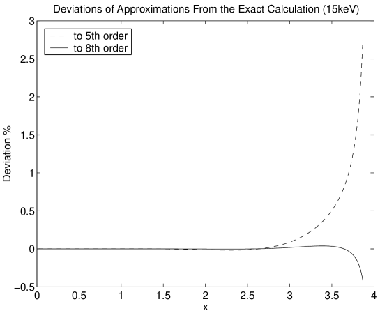
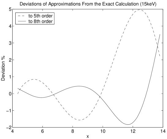
Figure 1: The deviations of the fifth (Itoh et al. 2000a) and eighth order approximations (equation 23) from the exact result.

References

• \harvarditem Birkinshaw, M., 1999, Phys.Rep., 310, 97-195. \harvarditem Carlstrom, J. E., Holder, G. P., & Reese, E. D., 2002, Annu. Rev. Astron. Astrophys., 40, 643-680. \harvarditem Challinor, A., Lasenby, A., 1998, ApJ., 499, 1-6. \harvarditem Chandrasekhar, S., Radiative Transfer (New York: Dover), 1950. \harvarditem Dolgov, A. D., Hansen, S. H., Pastor, S., & Semikoz, D. V., 2001, ApJ., 554, 74-84. \harvarditem Itoh, N., Kawana, Y., Nozawa, S., & Kohyama, Y., 2001, MNRAS, 327, 567-576. \harvarditem Itoh, N., Satoshi, N., astro-ph/0307519. \harvarditem Kompaneets AS., 1957,Sov.Phys.JETP, 4, 730-737. \harvarditem Molnar S.M., Birkinshaw M., 1999, ApJ., 523, 78-86. \harvarditem Nozawa S., Itoh N., Kohyama Y., 1998, ApJ., 502, 7-15. \harvarditem Nozawa, S., Itoh, N., Kohyama, Y., 1998, ApJ., 508, 17-24. \harvarditem Nozawa, S., Itoh, N., Kawana, Y., Kohyama, Y., 2000, ApJ., 536, 31-35. \harvarditem Rephaeli Y., 1995, Annu. Rev. Astron. Astrophys.., 33, 541-579. \harvarditem Rephaeli Y., 1995, ApJ.., 445, 33-36. \harvarditem Sazonov S.Y., Sunyaev R.A., 1998, ApJ., 508, 1-5. \harvarditem Sunyaev RA, Zeldovich YB., 1972, Comments.Astrophys.Space Phys., 4, 173-178. \harvarditem Sunyaev R.A., Zel’dovich Y.B., 1980, MNRAS, 190, 413-420. \harvarditem Wright EL, 1979, ApJ., 232, 348-351.
• [1]
Refer to caption
Refer to caption