The Canada-UK Deep Submillimeter Survey VII: Optical and Near-Infrared Identifications for the 14^h  Field

Abstract

We present the multi-wavelength identifications for 23 sources in the Canada-UK Deep Submillimeter Survey (CUDSS) 14^h  field. The identifications have been selected on the basis of radio and near-infrared data and we argue that, to our observational limits, both are effective at selecting the correct counterparts of the SCUBA sources. We discuss the properties of these identifications and find that they are very red in near-infrared color, with many classified as Extremely Red Objects, and show disturbed morphologies. Using the entire CUDSS catalogue of 50 sources we use a combination of spectroscopic redshifts (4 objects), 1.4GHz-to-850$\mu$m flux ratio redshift estimates (10 objects), and redshift lower-limits based on non-detections at 1.4GHz (the rest of the sample) to estimate a lower-limit on the median redshift of the population of $z_{med}>$ 1.4. Working from simple models and using the properties of the secure identifications, we discuss general and tentative constraints on the redshift distribution and the expected colors and magnitudes of the entire population.

1 Introduction

The submillimeter surveys of the last five years, using the Submillimeter Common-User Bolometer Array (SCUBA) and the Max-Planck Millimeter Bolometer array (MAMBO) (Smail, Ivison, & Blain, 1997; Barger et al., 1998; Hughes et al., 1998; Eales et al., 1999; Borys et al., 2002; Cowie, Barger, & Kneib, 2002; Scott et al., 2002; Dannerbauer et al., 2002) have revealed a population of high-redshift objects which play an important role in the formation and evolution of galaxies. Though relatively rare ($\sim$0.5 arcmin^-2 at $S_{850{\mu}m}>$ 3 mJy) these systems have extreme individual luminosities ($>$ 10¹² L_⊙) and are responsible for $\sim$ 20% of the far-infrared background at 850$\mu$m (to $S_{850{\mu}m}>$ 3 mJy) (Blain et al., 1999; Barger et al., 1999a; Cowie, Barger, & Kneib, 2002; Scott et al., 2002; Webb et al., 2003b). This is in striking contrast to the relative unimportance of similar far-infrared bright galaxies in the local universe (see Sanders & Mirabel (1996) for an extensive review), and indicates substantial evolution in this population with redshift. The high star formation rates of these galaxies of $\sim$100-1000 M_⊙/year, are sufficient to produce a massive galaxy over a dynamical timescale, and make them strong candidates for the progenitors of local elliptical galaxies. However, there are still many unanswered questions regarding the nature of these objects, their redshift distribution, and their relationship to other high-redshift populations.

A key issue, but one of the hardest to address, is the nature of the obscurred energy source. Determining the fraction of energy produced by star-formation and active galactic nuclei (AGN) is crucial for understanding how these systems fit into theories of galaxy evolution (e.g. Archibald et al. (2002)). Though a number SCUBA sources which have been studied in detail show signs of AGN activity, and indeed, all SCUBA sources may be home to obscured AGN, the current evidence points toward star-formation dominated systems (Frayer et al., 1998, 1999; Barger et al., 1999b, 2001; Smail et al., 2002; Ivison et al., 2002; Waskett et al., 2003; Almaini et al., 2003; Alexander et al., 2003). Even once the relative contribution of an AGN to the submillimeter flux is known, inferring a star formation rate is still difficult. The primary uncertainty results from the poorly understood dust temperature in these systems and though we may attempt to calibrate this using $z\sim$0 ULIRGs (Dunne, Clements, & Eales, 2000a; Yun & Carilli, 2002), there is growing evidence that these local objects may not be representative of the high-redshift SCUBA sources (e.g. Ivison et al. (2001); Lutz et al. (2001); Frayer et al. (2003)). An understanding of the energy production and radiation mechanisms in these systems will require extensive follow-up observations, with a level of detail similar to those of Lutz et al. (2001),Ledlow et al. (2002),Genzel et al. (2003),and Frayer et al. (2003) for many systems. The speed with which we can carry-out these observations is limited by current technology but this will change dramatically with future facilities such as ALMA, JWST, and the LMT.

Though these systems certainly have sufficient star formation rates to rapidly form an elliptical galaxy, it is less clear that their spatial density (e.g. Fox et al. (2002)) and clustering properties (Ivison et al., 2000a; Scott et al., 2002; Webb et al., 2003b) are consistent with local massive elliptical galaxies. This would be an evolutionary link between the two populations, but requires a complete determination of the redshift distribution, and in particular, for a measure of the clustering strength, significant sky coverage. Such measurements would also shed light on the relationship between these objects and other high-redshift populations. Though the Lyman-break galaxies have very little direct overlap with the bright submillimeter population ($S_{850{\mu}}\mathrel{\hbox{\hbox to0.0pt{\hbox{\lower 4.0pt\hbox{$\sim$}}\hss}\hbox{$>$}}}$ 3 mJy), they are likely present at significant numbers in the fainter $S_{850{\mu}m}$ counts (Peacock et al., 2000; Chapman et al., 2000; Webb et al., 2003a). There is also tentative evidence that the LBGs and SCUBA sources may trace the same large scale structure (Webb et al., 2003a), perhaps forming a mass sequence in which SCUBA sources represent the most massive star forming systems at high-redshift(Magliocchetti et al., 2001; Granato et al., 2001; Genzel et al., 2003), or alternatively, they may be related through time, as systems evolve from a dusty, luminous stage of intense star formation though a relatively dust-free and perhaps extended phase of moderate star formation. (Shapley et al., 2001; Ivison et al., 2002).

The determination of the redshift distribution is hindered by the uncertainties in the source positions, due relatively large beam size of the JCMT at 850$\mu$m. Positions are generally secured through radio detections which biases the measured redshifts to $z\lesssim$ 3 (Chapman et al., 2003). A further possible complication is the different flux limits reached by different surveys, ranging from the sub-mJy limits of the cluster surveys (Smail, Ivison, & Blain, 1997; Chapman et al., 2002) to the very bright ($S_{850{\hbox{$\mu$m}}}>$ 8mJy) limits of the ’8 mJy survey’ (Scott et al., 2002). There are indications that the brighter SCUBA sources may lie at predominantly higher-redshifts than the fainter systems (Chapman et al., 2002; Ivison et al., 2002). If so, relatively deep surveys such as this one would be biased to lower-redshift sources compared to shallower programs such as the “8 mJy Survey” (Scott et al., 2002; Fox et al., 2002; Ivison et al., 2002).

The resolution of all of these issues requires the careful and extensive follow-up of a wide variety of sources, over a range of flux levels and selection techniques. Unfortunately, the first step of identifying the optical counterparts of these systems is not trivial and many SCUBA sources catalogued in current surveys have no solid identification (Fox et al., 2002; Smail et al., 2002; Ivison et al., 2002; Webb et al., 2003b). This is a result of the uncertainty in the submillimeter positions and the faint and red nature of these objects at optical wavelengths (e.g. Frayer et al. (2000a); Lutz et al. (2001); Dunlop et al. (2002); Dannerbauer et al. (2002)). Hence, more than one candidate identification often lies within a given submillimeter error radius. Even once counterparts have been securely identified they are typically so faint that optical and near-IR spectroscopic redshifts can only be measured with 8-m class telescopes (if at all) and large investments of observing time are required (e.g. Barger et al. (1999b); Chapman et al. (2003). This situation will improve with the commissioning of facilities which will measure redshifts through masers, CO lines, and far-IR photometry, and will not require bright optical/NIR counterparts (Combes, 1999; Hughes et al., 2000; Frayer, 2001; Townsend et al., 2001; Hughes et al., 2003; Aretxaga et al., 2003)

It is because of the empirical correlation between radio and far-infrared flux (Carilli & Yun, 1999; Dunne, Clements, & Eales, 2000a; Yun & Carilli, 2002), and the excellent resolution of large radio arrays, that radio mapping currently offers the best chance to secure positions of the sources. Moreover, the extremely low surface density of radio sources makes chance coincidences between the radio and submillimeter populations highly unlikely. Unfortunately, at the current typical flux limits radio detections are biased to redshifts of z $\lesssim$ 2-3 and, depending on the redshift distribution of the SCUBA sources, may miss a substantial fraction of the population (Eales et al., 2000; Chapman et al., 2002; Ivison et al., 2002; Webb et al., 2003b). NIR imaging is crucial as these objects may be expected to be very red due to the presence of dust (but also see Trentham et al. (1999)). Indeed, a significant fraction of SCUBA sources have been associated with Extremely Red Objects (EROs) or Very Red Objects (VROs) (Dey et al., 1999; Gear et al., 2000; Smail et al., 1999; Fox et al., 2002; Ivison et al., 2002; Dannerbauer et al., 2002; Dunlop et al., 2002). As in the radio, the relatively low surface density of red objects, compared to optically selected populations, reduces the frequency of chance positional coincidences.

In this paper we explore the multi-wavelength properties and redshift distribution of submillimeter sources detected in the Canada-UK Deep Submillimeter Survey (CUDSS). We present the identifications for sources in the 14^h  field and discuss the properties of the entire catalogue. Here we briefly re-cap the previous papers which have resulted from this survey. The submillimeter data are discussed in detail in Eales et al. (1999, 2000) (Papers I and IV) and Webb et al. (2003b) (Paper VI). The first identifications were presented in Lilly et al. (1999) (Paper II). One of our brightest sources CUDSS 14.1, which has been observed extensively at other wavelengths, is discussed in Gear et al. (2000)(Paper III). A discussion of the submillimeter properties of Lyman-break galaxies in the survey fields may be found in Webb et al. (2003a) (Paper V). The optical/NIR identifications of the 3^h  field are presented in Clements et al (in preparation).

This paper is organized as follows. In §2 we outline the multi-wavelength data which we, and others, have obtained over this field area. §3 explains our procedure for identifying counterparts and presents the identifications. In §4 we discuss the properties of individual sources. In §5 contains a discussion of our results in detail. Finally, in §6 we summarize our results. We assume a flat, $\Lambda$=0.7 cosmology and H_∘=72 km/s/Mpc throughout.

2 The multi-wavelength data

2.1 The submillimeter observations

The CUDSS Survey consists of two primary fields: the 14^h  field (48 arcmin²) and the 3^h  field (60 arcmin²). These fields are contained within the Canada-France Redshift Survey (CFRS) fields CFRS14+52 and CFRS03+00 respectively. The submillimeter data were obtained using SCUBA on the JCMT over many observing runs from 1998 to 2001. The details of the submillimeter observations are discussed in Papers IV and VI. Paper VI also contains the complete 3^h  field catalogue of 27 sources.

In Paper IV we presented a source catalogue for the 14^h  field of 19 objects with $S/N\geq$ 3. Since then we have acquired new submillimeter data, primarily located on the upper strip of the field which, previously, had not been imaged to the same depth as the rest of the field. Through the addition of these data four new sources were detected, all at $S/N\sim$ 3. These new observations marked the completion of the submillimeter survey of this field and we now present our final catalogue in Table 1. Note that sources 14.1 through 14.19 are identical to the sources listed in Paper IV.

2.2 Radio and ISO Data

Most of the $14^{h}$ field has been mapped at 1.4 GHz and 5 GHz by Fomalont et al. (1991) to a depth of $\sim 16~{}\mu$Jy and 2.5 $\mu$Jy, respectively. Data at 1.4 GHz also exists for the 3^h  field (Yun personal communication; Ivison personal communication) and was discussed in Paper VI. Taking advantage of the improved wide field imaging algorithms in the AIPS software system, M. Yun re-calibrated the archival VLA data by Fomalont et al. and obtained a new continuum image with about twice the improved resolution ($\theta_{FWHM}\sim 4\hbox{${}^{\prime\prime}$}$) using a robust weighting of visibilities. The final dynamic range limited noise in the 14^h  image is $14\mu$Jy, similar to that of Fomalont et al. As a comparison to other surveys we note that the ratio of the submillimeter to radio 1$\sigma$ noise level (per beam) in this survey is 1mJy/14$\mu$Jy $\sim$ 70, while for the HDF it is 0.4mJy/7.5$\mu$Jy $\sim$50 (Hughes et al., 1998; Richards, 2000) and for the ’8 mJy survey’ it is 2mJy/4.8$\mu$Jy $\sim$ 400 (Scott et al., 2002; Ivison et al., 2002).

In addition to the improved angular resolution, completely different noise characteristics and a different treatment of a serious imaging problem make the examination of the newly reduced 1.4 GHz image worthwhile. Because these VLA observations are done in the continuum mode, both the 1.4 GHz and the 5 GHz images suffer from beam smearing (chromatic aberration) – cross-correlation of signal with different wavelengths with the bandpass causes a loss of amplitude and displacement of source position in a radial direction from the phase center (see Bridle & Schwab 1988). This problem is particularly severe for the SCUBA sources because they are located mostly outside the central 150^′′ region which is relatively problem-free. Fomalont et al. dealt with this problem by summing all flux over the radially elongated source regions (E. Fomalont, private communication in 2000). Recovering the total flux this way requires summing over more than one beam areas (thus increasing noise) and may not fully account for the amplitude de-correlation. Instead, we have measured the peak amplitudes from the image and then recovered the source flux using the correction factor that depends on the radial distance from the phase center using Eq. 13-24 in Bridle & Schwab. The new location and the recovered flux density for the SCUBA sources in the 14^h field are given in Table 2. The new 1.4 GHz image does not yield any new detections of the SCUBA sources within the search radius of 8^′′, but we can derive a more accurate upper limits after properly taking into account the effects of beam smearing.

Both SCUBA fields have been imaged by the Infrared Space Observatory (ISO). The data covering the 14^h  field at 7$\mu$m and 15$\mu$m are discussed in detail in Flores et al. (1999a, b). The data covering the 3^h  field are not yet published and have been provided to us by Hector Flores.

2.3 Existing Optical Data: The CFRS and HST

The CFRS fields have been extensively studied at optical wavelengths. In addition to the original $UBVIK$ photometry and spectroscopic redshifts ($z\leq$ 1.3) of the CFRS itself (Lilly et al, 1995b; Hammer et al., 1995a), Hubble Space Telescope (HST) $VI$ imaging was undertaken for CFRS morphology follow-up work and further archival observations were available (see footnote 1, first page).

2.4 New HST Data

As part of follow-up work for this survey we acquired three new $I$-band HST pointings for each CUDSS field. These data were reduced and calibrated using the general HST reduction pipeline and reach an $I_{AB}$ depth of $\sim$26.0 mags. These data, combined with the existing HST data described above, cover 19/23 objects in the 14^h  field, and 19/27 objects in the 3^h  field.

2.5 New Near-Infrared Data: Kitt Peak and CFHTIR

The $K$-band imaging of the CFRS was extremely shallow and covered only 1/3 the CFRS fields fields. Thus, we obtained new $K$-band imaging using IRIM on the Mayall-4m at Kitt Peak and using the CFHTIR camera on the CFHT. The CFHTIR data have better pixel resolution than the IRIM data, with 0.207 arcsec/pixel, versus 0.6 arcsec/pixel, as well as improved sky quality. The Kitt Peak data reach a depth of $K_{AB}\sim$21.5 mags and the CFHTIR data reach $K_{AB}\sim$22.5-23.0 mags, over most of the image. Both data sets cover roughly 2/3 of the 14^h  and 3^h  fields.

3 The Multi-wavelength Identifications

3.1 The Identification Procedure

We have chosen a method which selects counterparts on the basis of positional coincidence (Downes et al. (1986); Paper II) as follows. The probability that an object, physically unrelated to a given SCUBA source, will lie within a distance $r$ of said source can be described by $P=1-exp(-{\pi}nr^{2})$, where $n$ is the surface density of galaxies as bright or brighter than the candidate identification. Defined in this way, the lower the $P$ value, the higher the statistical significance of the identification.

As pointed out in Paper II, using the surface density of objects as bright or brighter than the candidate identification inherently underestimates the probability of random associations. This is because one effectively searches many independent galaxy samples simultaneously, and the chance that one of these samples will produce an identification of high significance is increased. We must, therefore, calculate a new quantity $P^{\prime}=\alpha P$, where $\alpha$ is determined from Monte-Carlo simulations of our identification procedure. We use randomly chosen positions in place of real SCUBA positions, which yields an empirical estimate of the probability of finding a galaxy of a given magnitude and color within the search radius of a random position.

These $P^{\prime}$ values should be interpreted in the following way. If we assume that SCUBA sources are completely unrelated to the optical/near-IR population within which we search for identifications, we would statistically expect to select 10 identifications with $P^{\prime}\leq$ 0.1 for every 100 SCUBA sources. Thus, $P^{\prime}$ for a single identification should be interpreted with respect to the entire sample, rather than in isolation.

We have empirically estimated our search radius by placing and recovering fake SCUBA sources in our submillimeter map, and through Monte-Carlo simulations of the data (Paper IV). We found the positional offset between the measured position of an object and its true position was $\leq$ 8^′′  90-95% of the time, and therefore we use this as our search radius. This is a larger search radius than used by some groups (e.g. Barger et al. (1999b); Smail et al. (2002)) though we note that the peak of our offset distribution lies at a smaller radius of 2-4^′′ (also see Hogg (2001)).

3.2 The Radio and Mid-Infrared Identifications

In Paper IV we presented five radio identifications for the 14^h  field and these are listed in Table 2, along with their $P$ statistics. At these levels of significance we do not expect any of these five identifications to be the result of random SCUBA-radio associations. In Table 2 we also include a possible radio counterpart for source 14.19 which lies beyond our search radius. As we expect 1-2 identifications (for our sample size) with offsets from the SCUBA position of $>$ 8^′′, this identification should be considered but is by no means secure.

The ISO identifications were also discussed in Paper IV and are summarized in Table 3. Three sources have been detected in the mid-IR, two of which (14.13, 14.18) are also coincident with radio emission. The third detection (14.17) has a very large offset (10.3^′′) and is therefore not a secure identification.

3.3 The Near-Infrared Selected Identifications

In Paper II the identifications were chosen from an $I$-selected population. In this work we have improved our algorithm by including $K$ information as follows. For a given $K$-selected galaxy within the positional error radius of a SCUBA source we compute the surface density of galaxies as bright or brighter than its $K$-band magnitude and as red or redder than its $(I-K)$ color, directly from our CFHTIR mosaic image and the CFRS optical data. Because we estimate this directly from the follow-up data field-to-field variations in density are taken into account.

Using the $(I-K)$ color is advantageous for two reasons: (1) Since red galaxies have a lower surface density than galaxies of more moderate color the chance of random coincidences is decreased, and (2) Because SCUBA sources are by their nature very dusty we may begin with the reasonable assumption that they have redder colors than the typical galaxy. This second point is somewhat contentious since bright submillimeter flux does not necessarily guarantee red optical/NIR colors. In fact, Trentham et al. (1999) has shown that some low-redshift ULIRGs have surprisingly blue optical colors when placed at high-redshift.

$P^{\prime}$ was calculated for each $K$-selected galaxy within 8^′′  of each SCUBA source. This was done blindly with respect to the radio and mid-infrared data. All 23 SCUBA sources had at least one candidate identification within their submillimeter error radius (i.e. there were no demonstratable “empty fields”), and there were typically 1-3 possibilities. Table 4 lists the best identification (i.e. the one with the lowest $P^{\prime}$ value) for each source.

In Figure 1 we plot a histogram of the $P^{\prime}$ values for the SCUBA identifications (solid line) and for the Monte-Carlo simulations of our identification procedure (dashed line). An excess of real identifications with $P^{\prime}$$\leq$ 0.1 over the number predicted by the Monte-Carlo simulation is apparent. Statistically we expect two random associations at this level of significance but our procedure has selected seven. This implies that on order five of these seven sources are correctly identified.

One might expect that the addition of radio information to the NIR data would solidify a number of ambiguous identifications, but we find this is not the case. Of the seven NIR-selected identifications with $P^{\prime}<$ 0.1, five of them are the same identifications selected by radio detections. That is, given only the NIR data our identification procedure securely identifies the same objects that are identified using radio data. Therefore, at these flux limits (14 $\mu$Jy) the radio data do not greatly improve the identifications over the NIR data. In particular it does not identify objects missed by the NIR algorithm.

Between $P^{\prime}$$\sim$ 0.1 and $P^{\prime}$$\sim$ 0.5 there is still an excess over random but it is less pronounced, only $\sim$ 3 sources. Thus, in this region it is reasonable to expect a number of correct identifications but there are at least as many, and probably more, random associations. Moreover, it is impossible to know which specific identifications are correct simply based on the $P^{\prime}$ value.

One might worry that our identification algorithm will be overly biased toward red identifications but this appears to have a negligible effect. In Figure 2 we show the magnitudes and colors of the identifications selected when the algorithm is run with random positions in place of SCUBA positions. In this case the best identifications posses a wide range of magnitudes and colors and are not concentrated in the region in which the good SCUBA identifications are located. There is a small offset towards redder average color for a given magnitude but this is not large enough to account for the unusually red colors of the statistically secure identifications. Also shown in Figure 2 are the colors and magnitudes of the Monte Carlo identifications found when we modify our identification algorithm to be biased toward blue objects, rather than red. Again, the colors of the selected identifications span a wide range of values and are only offset by a small amount from the color of the general field population.

3.4 Lyman-break galaxy identifications

This field has also been surveyed for Lyman-break galaxies (LBGs) by two groups: Steidel and collaborators (personal communication) and the Canada-France-Deep-Fields Survey (CFDF) (McCracken et al. (2001); Foucaud et al., in preparation). The statistical submillimeter properties of the LBG population within the CUDSS fields has been explored by Webb et al. (2003a), who also discuss the two LBG samples in detail. In this work we will limit the discussion to SCUBA sources with possible LBG counterparts.

As with red galaxies and radio sources LBGs have low surface densities and are therefore less likely to be randomly associated with SCUBA sources. There are five LBGs within 8^′′ of a SCUBA source and these are listed in Table 5. However, one of these is within the error radius of source 14.9 and, as 14.9 is securely identified with a radio source, the LBG is clearly a positional coincidence.

The remaining LBG identifications are not secure for the following reasons. Given the $P$ values of the CFDF LBG identifications we would expect about one random association. There are two (sources 14.6 and 14.9) and therefore based purely on this one could conclude that 14.6 is properly identified with an LBG. However, as this is only an excess of one object over that expected randomly it is not statistically significant. The $P$ values of the Steidel et al. identifications are all too high to be considered secure. At these levels of significance we would expect two such identifications randomly and we have three. Again, this is an excess of only one object of the number expected randomly and well within the shot noise.

To estimate the $P$ statistic for these objects the surface density of LBGs over the entire survey field was used but, in fact, these four objects are found amongst the densest concentration of LBGs in this field. This could have a number of interpretations. It is most likely these identifications are simply chance coincidences occurring with greater frequency because of the higher surface density of objects in this region. However, submillimeter sources have been associated with regions of optical over-densities (Chapman et al., 2001) and indeed, this small area within the survey field also contains the highest concentration of SCUBA sources in our survey. Perhaps more LBGs in this region are submillimeter bright because of high-density environment effects, or this area is an over-dense region in real-space where the SCUBA sources and LBGs are clustered together but not physically the same objects (Webb et al., 2003a).

3.5 The Positional Offsets

In this section we consider four positional offset distributions of interest. These distributions are shown in Figure 3 and discussed below.

1. Figure 3(a). The offsets derived in the Monte-Carlo simulations of the identification procedure. These are the offsets between the random positions chosen from the $K$-image and the best “fake” identification chosen for each random position. This is the distribution that the incorrect identifications will follow. These are not uniformly distributed, but peak at 7^′′, with very few at low offsets.

2. Figure 3(b). The distribution of offsets between the measured and true positions of objects in the submillimeter data due to the effects of noise and confusion. These are the offsets that the real SCUBA sources and their true counterparts would be expected to follow. As outlined in §3.1 and Paper IV, this was estimated through simulations of the submillimeter data. This distribution peaks at $\sim$2-3^′′ with an extended tail to large offsets.

3. Figure 3(c). The offsets between the submillimeter positions of the real SCUBA sources and their best NIR-selected identification. Clearly this distribution will be a superposition of the above two distributions, (a,b), as the identifications are a mixture of true counterparts and incorrect identifications. Indeed, if one compares Figure 3(c) with Figure 3(a), an excess of offsets at $<$ 5^′′ is evident. The magnitude of this excess is roughly equal to the excess number of objects over random found by the NIR identification algorithm (Figure 1).

4. Figure 3(d). The offsets between the submillimeter positions and the radio positions for the SCUBA sources detected in the radio. These are secure identifications and thus these offsets mirror the offsets of (2). To clearly show the distribution we have included the radio sources from both CUDSS fields (see Paper VI).

4 Notes On Individual Sources

Below we discuss the properties of individual identifications. Based on the reasoning discussed in the previous sections we have divided our sample into three identification categories: (1) those with radio detections (all but one are considered secure), (2) those with plausible identifications and, (3) those with ambiguous or poor identifications.

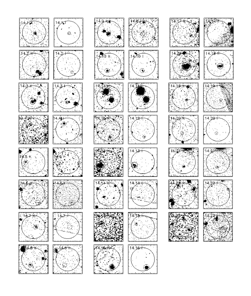
Figure 4: The $K$ (left of pair) and $I$ (right of pair) images (20^′′$\times$20^′′) of all 23 sources in our 14^h  catalogue, centered on the submillimeter position. The large circle denotes the 8^′′search radius, or 90-95% confidence region. The smaller circles mark the best NIR-selected identification for each source. Solid circles correspond the objects which have also been detected at 1.4GHz, while dashed circles mark non-radio sources. North is up and east is to the left.

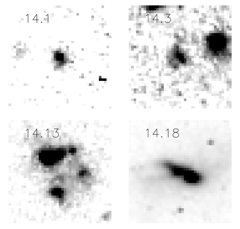
Figure 5: HST $I$-band images of the four radio sources with HST imaging. The images are 4$\times$4 ^′′. North is up and east is to the left.

In the following discussion we define an ERO as objects with $(I-K)_{AB}\geq$ 2.7 and a VRO as objects with $(I-K)_{AB}\geq$ 2.2 . Postage stamp images (20^′′$\times$ 20^′′) in $I$ and $K$ of the SCUBA sources are shown in Figure 4, and HST $I$-band images of the four radio identifications with HST imaging are shown in Figure 5.

We also discuss the redshift or redshift constraints for many of the sources. When, as in most cases, spectroscopic measurements are not available we have estimated the redshift using the FIR and radio data (Yun & Carilli (2002), hereafter referred to as the YC method) and NIR/optical colors (see §5). Yun & Carilli (2002) used the entire radio-to-FIR SED to derive a photometric redshift and should therefore be a superior method to the 1.4GHz-to-850$\mu$m flux ratio method which only uses two data points (but see also Blain, Barnard, & Chapman (2003) for caveats). The assumed template SED was produced by Yun & Carilli from the observations of 23 local dusty starburst galaxies which span an order of magnitude in SFR and $L_{FIR}$.

4.1 The Radio Sources

CUDSS 14.1

This is the brightest object in our 14^h  field sample has been extensively studied at 1.4 GHz, 5 GHz, 1.3 mm, optical ($VI$) and near-IR ($JHK$) wavelengths (Fomalont et al., 1991; Gear et al., 2000). It is classified as an ERO with with $(I-K)_{AB}$ = 3.6. The HST $I$-band image shows asymmetrical morphology (Figure 5).

Using the YC method we estimate a redshift of $z$=2.3 $\pm$ 0.5 with a star formation rate of 635 M_⊙/year or $L_{FIR}$ = 3.7$\times$10${}^{12}L_{\odot}$ (Kennicutt, 1998) (Figure 6). This is in good agreement with earlier estimates of the redshift (Gear et al., 2000). Assuming this source has a similar optical/NIR SED to source 14.13 (which is also well studied and has a spectroscopically determined redshift) places it in the range $z\sim$ 2.4-3.7.

CUDSS 14.3

This object is identified with a radio source 15V23 (Fomalont et al., 1991). It has a color of $(I-K)_{AB}$=2.4 and is classified as a VRO. Though the object is faint, the HST $I$-band image clearly shows asymmetrical morphology (Figure 5).

Following the YC method we estimate a redshift of $z$=1.7 $\pm$ 0.5 with a star formation rate of 315 M_⊙/year (Figure 6) or $L_{FIR}$ = 1.8$\times$10${}^{12}L_{\odot}$ (Kennicutt, 1998). Using source 14.18 as a NIR template constrains this source to $z\sim$ 1.3-2.5.

CUDSS 14.9

This object is securely identified with radio source 15V67 (Fomalont et al., 1991) with $(I-K)\mathrel{\hbox{\hbox to0.0pt{\hbox{\lower 4.0pt\hbox{$\sim$}}\hss}\hbox{$>$}}}$ 4.0 (it is undetected in the CFRS $I$-band image and no HST imaging exists in this region). It is one of a chain of three extremely red objects ($(I-K)_{AB}$=3.48 and $(I-K)_{AB}\mathrel{\hbox{\hbox to0.0pt{\hbox{\lower 4.0pt\hbox{$\sim$}}\hss}\hbox{$>$}}}$4.1), that is 10^′′ long. The YC redshift estimate is $z$=1.6 $\pm$ 0.6, and a star formation rate of 265 M_⊙/year or $L_{FIR}$ = 1.5$\times$10${}^{12}L_{\odot}$ (Kennicutt, 1998) (Figure 6).

CUDSS 14.13

This source is securely identified with radio source 15V23 (Fomalont et al., 1991) also known as ISO 0 (Flores et al., 1999a) and CFRS 14.1157 (Hammer et al., 1995b). It has $(I-K)_{AB}$=2.6 and is classified as a VRO. The HST imaging shows an extended object ($\sim$2.5^′′) with multiple components separated by diffuse emission (Figure 5).

This object has a spectroscopic redshift (Hector Flores, personal communication) of $z$=1.15. Using the YC method we find $z$=1.3 $\pm$ 0.4 with a star formation rate of 195 M_⊙/year or $L_{FIR}$ = 1.1$\times$10${}^{12}L_{\odot}$ (Kennicutt, 1998)(Figure 6). This source has recently been detected at x-ray wavelengths (Waskett et al., 2003), and likely contains an AGN.

CUDSS 14.18

This is the faintest object (at 850$\mu$m) in this catalogue and is located in the deepest region of our map. It is identified with radio source 15V24 (Fomalont et al., 1991) also known as ISO 5 (Flores et al., 1999a) and CFRS 14.1139 (Lilly et al, 1995a). HST imaging shows disturbed morphology (Figure 5).

It has a spectroscopic redshift of $z$=0.66 (Lilly et al, 1995b). The YC redshift estimate places this objects at $z$=1.0$\pm$ 0.3 and a star formation rate of 165 M_⊙/year or $L_{FIR}$ = 1.0$\times$10${}^{12}L_{\odot}$ (Kennicutt, 1998).

CUDSS 14.19

This source has a radio detection at 8.5^′′, just beyond the search radius. We expect 5-10% of the sample to have identifications that lie beyond 8^′′ and so this identification is possible but by no means secure. A second possible identification is found with the NIR identification algorithm, which lies at a smaller offset of 3^′′ but is not statistically significant.

4.2 Plausible Identifications

The sources discussed in this section do not have radio detections. However, we know that a number of the non-radio sources have been correctly identified (§3) though it is not possible to know which ones simply based on their $P^{\prime}$ values. In the following we discuss three sets of identifications:

1. Sources with NIR-determined $P^{\prime}$$\leq$ 0.1 which do not have radio detections: sources 14.23 and 14.11. As discussed in §3 we expect $\sim$ 2 identifications due to positional coincidence at this level of significance. However, since we are dealing with small number statistics it is possible that none or both of these identifications are correct.

   CUDSS 14.11

   This object is best identified with a very bright object ($I_{AB}$=17.3) with $(I-K)_{AB}$ = -0.05. The lack of a radio detection for this source constrains its redshift to $z>$ 1.1. However, the optical identification has colors and morphology consistent with a low-redshift elliptical and this is, therefore, unlikely to be the correct identification. An alternative explanation (see next section), which is consistent with the radio-estimated redshift lower-limit, is that it is a foreground gravitational lens which is amplifying a submillimeter-bright object at higher redshift.

   CUDSS 14.23

   This object is identified with an ERO, with $(I-K)_{AB}$=3.6. As we discuss in §5, this source as NIR colors consistent with the radio detected objects if placed at redshifts of 2.5-3.7, and therefore this identification is considered likely.

2. Sources with LBG associations: These identifications were outlined in §3.4, and we concluded that none of the 4 LBG identifications could be considered secure. We discuss only one identification of interest.

   CUDSS 14.7

   The best identification for this object is the Steidel et al. LBG West2 MMD13, which is a spectroscopically confirmed QSO at $z$=2.913. It lies in the single most over-dense region of the Steidel et al. 14-hour LBG survey. There is a second possible identification in this field which at a comparable level of significance. This galaxy, at an offset of 2.1^′′, has an $(I-K)_{AB}\mathrel{\hbox{\hbox to0.0pt{\hbox{\lower 4.0pt\hbox{$\sim$}}\hss}\hbox{$>$}}}$ 2.8, thus is an ERO. Because there is no $I$ detection we only have an lower limit on the color and therefore an upper limit on the $P^{\prime}$ value and may therefore be of higher significance than the LBG.

3. Sources with NIR-determined $P^{\prime}$$>$ 0.1: In §3.3 we claimed that there was an excess of 3 identifications at this level of significance, over that expected randomly, and therefore at least this number of identifications are correct. Again, it is not possible to identify which sources have been correctly identified based solely on their $P^{\prime}$ values. Below we discuss those objects with interesting properties such as extremely red colors.

   CUDSS 14.2

   The best identification for this object is a very red galaxy 5.6 ^′′ away from the submillimeter position. Two arcseconds away from this identification (7.8^′′ from the submillimeter position) there is a second red object. These two objects are both classified as EROs and have colors of $(I-K)_{AB}$=3.5 and $(I-K)_{AB}$=3.7 respectively.

   CUDSS 14.5

   This object is best identified with a faint ($K_{AB}$=22.3) ERO ($(I-K)_{AB}$=2.7) at an offset of 5^′′. It is just detected in the CFRS $I$-band image and unfortunately, no HST data exists in this region.

   CUDSS 14.17

   This source is identified with ISO 195 (Flores et al., 1999a) which lies at an offset of 10.3^′′. Though larger than our nominal search radius we do expect 1-2 sources to have identifications with offsets from the submillimeter position of $>$ 8^′′. However, at such large distances the number of random coincidences rises significantly. This object has no spectroscopic redshift and cannot be ruled out by the radio redshift lower limit of $z>$ 1.6.

4.3 Gravitational lensing effects

The possibility that a significant fraction of SCUBA sources in blank-field surveys could be lensed by foreground objects was first discussed by Blain (1996) before the commissioning of SCUBA. Since then, a number of SCUBA sources that were (or would be) identified with relatively nondescript low-redshift galaxies, based on positional coincidence arguments, have, upon further study, turned out to be more distant objects, possibly magnified by the foreground object which was originally thought to be the identification (Smail et al., 1999; Dunlop et al., 2002; Chapman et al., 2002).

In our own survey there are a number of sources whose best identification is with a low-redshift system ($z<$ 1), two in the 14^h  field (14.11 and 14.18) and four in the 3^h  field (3.8, 3.10, 3.15, 3.25; Webb et al. (2003b)). Since none of these identifications have been verified through the detection of CO it is possible that all six are incorrect. If so, their close proximity to the SCUBA positions may be the result of lensing. However, the available evidence suggests this is not the case but rather that we have located the correct identification for all but one of these objects.

These systems, with the with the exception of source 3.25 (which is faint, small and diffuse, and source 14.11, which is bright, large, and spheroidal) exhibit unusual morphology suggestive of merger activity. Five of the six sources (all but 14.11) have detections at 1.4GHz, coincident with the optical identification, and four of these (all but 3.25) have also been detected at 15$\mu$m. These detections strengthen the statistical argument that these objects have been correctly identified since the surface density of radio and ISO populations is relatively low. More importantly, these are exactly the signatures we would expect for lower redshift objects.

However, this doesn’t remove the possibility that the 1.4GHz and 15$\mu$m flux has been lensed and the geometry of the lens system is such that the observed offsets between the source and lens are within the astrometric errors. However, if this were the case we would expect the 1.4GHz-to-850$\mu$m flux ratio to yield a redshift estimate consistent with a distant background source. In fact, all but sources 14.11 and 14.18, have 1.4GHz-to-850$\mu$m flux ratios consistent with a low-redshift ($z<$ 1) system. Source 14.18 is estimated to lie at $z\sim$ 1.4$\pm$ 0.3, which is not so large a discrepancy from the spectroscopic redshift of $z$=0.66 that it could be considered clear evidence for lensing (see for example Dunlop et al. (2002)). An alternative scenario is that although the submillimeter source has been amplified, the radio and ISO emission belong to the foreground galaxy. In this case the SCUBA source could lie at very high-redshift but the 1.4GHz-to-850$\mu$m flux would produce an erroneously low-redshift. As outlined above (and in §3.2) this is possible but statistically unlikely. Thus we conclude that sources 3.8, 3,10, 3,15, 3.25 and 14.18 have been correctly identified with low-redshift systems.

Source 14.11, on the other hand, is very suggestive of lensing. Though the optical identification does not have a measured redshift its color, angular size, morphology, and apparent magnitude are all consistent with a low-redshift elliptical. Not only is it difficult to reconcile strong submillimeter emission with this object, its lack of a radio detection places it at $z>$ 1.1. It is likely, then, that this is not the correct identification. Whether or not it is actually a lensed system cannot be addressed by these data.

5 Discussion

The first part of this work was concerned with identifying the multi-wavelength counterparts of the sources in the 14^h  field. In the remaining sections we will discuss the general properties of the population and expand the discussion to include both the 14^h  and 3^h  catalogues.

There are a number of securely identified sources in both fields which have reliable redshift estimates and relatively well studied SEDs. We will uses these objects as templates to draw tentative conclusions about the nature of the counterparts of all the objects. We will argue that we have correctly identified $\sim$ 50% of the catalogue, and that the remaining unidentified sources are likely faint, red objects beyond the detection limits of this work.

5.1 The 3^h  Field Identifications

The radio and mid-IR identifications for the 3^h  field sources were presented in Paper IV, and the optical/NIR counterparts are discussed in Clements et al., (in preparation). Clements et al. employ a slightly different algorithm for identifying counterparts than this work and use $K$-band images using UFTI camera on the UKIRT telescope as the primary NIR data set. In order to directly compare the identifications of the 3^h  field sources with those of the 14^h  field we have repeated the above 14^h  field identification analysis on the 3^h  sources using the CFHTIR data. This analysis produces a list of candidate identifications in good agreement with those of Clements et al.

There are 11 3^h  field sources whose NIR identifications have $P^{\prime}$$\leq$ 0.1. Statistically, we expect about three of these to be due to chance coincidence and the remaining eight identifications to be correct. Working from the radio data, there are 9 sources in the 3^h  catalogue which have been detected at 1.4 GHz (11 mJy, 1$\sigma$), six of which are the same identifications as those selected by the NIR algorithm with $P^{\prime}$$\leq$ 0.1. Of the remaining three radio identifications two are still the best identification selected by the algorithm, but at a lower level of significance. The remaining source (3.17) is the only radio-detected source in our catalogue which does not have an optical/NIR counterpart to the depths of these data. Thus, based on comparison to the radio identifications, our NIR algorithm remains successful at selecting the correct counterparts in the 3^h  field. However, there may be a higher level of contamination (5/11) for the 3^h  field than for the 14^h  field (2/7), (if these are indeed incorrect identifications), two sources are not identified with confidence, and one is missed due to its faintness.

5.2 Properties of the identifications

In Figure 7 we show the $I$, $K$ and 1.4 GHz fluxes of five radio-detected objects as they would appear when placed at higher redshifts. These are sources 14.1, 14.13, 14.18, 3.10, and 3.15 which have measurements in at least four optical/NIR filters. Sources 14.13, 14.18, and 3.10 have spectroscopically measured redshifts, while for 14.1 and 3.15 we have assumed the radio-far-infrared redshift estimate. For the 3^h  field sources, which have only 1.4 GHz measurements, a spectral index typical of star forming galaxies was adopted: $S\propto{\nu}^{-0.5}$ (Fomalont et al., 1991).

A number of interesting conclusions may be drawn from this figure. Firstly, the optically faint natures of these objects do not require them to lie at very high-redshift. All of these objects reach $I_{AB}$ = 26 between $z\sim$ 1.3 (3.10) and $z\sim$ 3.5 (14.1). They are all visible at $K$ to higher redshifts than at $I$, but would drop out of our $K$ image between $z\sim$ 1.7 (3.10) and $z\sim$ 4.5 (14.1 and 14.13).

Secondly, all of these objects become undetectable at 1.4 GHz (to our 1.4 GHz limits) at significantly lower redshift than they do at $K$. For example, source 14.1 would drop out of the radio survey at $z\sim$ 3.3, while remaining visible at $K$ to $z\sim$ 4.5. Source 3.10 becomes undetectable at 1.4 GHz at $z\sim$ 0.5, while still visible at $K$ to $z\sim$ 1.7.

This has important consequences for the identifications. If these radio sources are appropriate templates for the entire population there should be no submillimeter sources in the sample which are detected in the radio but have no $K$-band counterpart to our limits. Indeed there are none in the 14^h  field and only one in the 3^h  field. Moreover, there will be counterparts with similar optical/NIR properties to the radio-detected objects, but which have no radio detection. We may use this fact to identify likely counterparts in the absence of radio information.

Figure 8 presents a NIR color-magnitude diagram for the best identification for each source in the 14^h  and 3^h  catalogues. The solid circles correspond to the identifications with radio detections, and the solid diamonds to those with $P^{\prime}$$\leq$ 0.1 but with no radio detection. The open symbols correspond to the best identification for each of the remaining SCUBA sources. For comparison the magnitudes and colors of all the galaxies in the CFHTIR 14^h  image are also shown (plus signs). The bulk of identifications with radio detections or with $P^{\prime}$$\leq$ 0.1 lie along the upper envelope of the general population, and are among the reddest objects at each magnitude

Overlaid on Figure 8 are two sets of tracks. The dashed lines show the extrapolated magnitudes and colors, as a function of redshift, for the five radio sources from Figure 7. Also shown (solid lines) are the predicted NIR colors and magnitudes for three ULIRGs studied by Trentham et al. (1999) as they would appear at higher redshifts. Though all three are ULIRGs they do not have consistent optical/NIR colors, particularly at high-redshift. In particular, IRAS F12112+0305 (the bluest track) remains relatively blue at all redshifts. Thus it is not a foregone conclusion that these objects must have very red optical/NIR colors because simply because they are dusty. Indeed, sources 3.6, 3.25, and 3.27 are much bluer than the other radio sources (albeit with large uncertainties on their color) and lie along the track of IRAS F12112+0305.

5.3 Constraining the non-radio counterparts

Many of the non-radio identifications lie along the extrapolated tracks of the radio counterparts Figure 8, indicating that they may be similar to the securely identified sources, but lie at higher redshifts. We can use this information to identify likely counterparts and estimate redshifts for roughly 50% of the sample.

We begin by discussing those objects with $P^{\prime}$$\leq$ 0.1 which do not have a radio detection. In the 14^h  field these are sources 14.11 and 14.23. Source 14.23 lies within the same region as sources 14.1, 14.3, and 14.9. In fact, it has the exact color and magnitude as source 14.13 if placed at $z$ = 3.1. Source 14.11, on the other hand, lies in the lower left corner of the plot with the bright, blue galaxies, far away from the radio sources. Based on this it is reasonable to conclude that source 14.11 is incorrectly identified while 14.23 is likely correct (see §4.3 for further arguments that 14.11 has not been correctly identified). The fact that source 14.23 has not been detected at 1.4 GHz is not worrying as source 14.13 would not be detected in the radio beyond $z\sim$ 1.2, though it would be visible at $I$ and $K$ to $z\sim$ 3.5 and $z\sim$ 4 respectively.

In the 3^h  field sources 3.2, 3.4, 3.5, 3.13, 3.16 have $P^{\prime}$$\leq$ 0.1 but do not have radio detections. Three of these (sources 3.4, 3.13, and 3.22) have colors consistent with radio sources at higher redshift, and we therefore take these to be the correct counterparts.

There are four sources (14.2, 14.5, 14.14, and 14.22) with $P^{\prime}$$>$ 0.1 and colors consistent with the radio identifications at higher redshifts. This is approximately the number of identifications expected over random associations at this level of significance.

To summarize, given the radio and ISO identifications and those NIR selected identifications deemed correct based on their location in the color-magnitude diagram we have identified likely counterparts for 50% of the sources in our submillimeter catalogue. Later in the paper we will argue that the remaining 50% are likely faint and red and lie below the detection limits of these data.

5.4 Data constraints on the redshift distribution

Simple redshift estimates may be made for objects based on optical/NIR and colours using the secure, well-studied, low-redshift identifications as templates. For each identification we find the template SED (Figure 7) and redshift that best describes the source’s NIR magnitude and colour. The resulting redshift estimates are listed in Table 6 along with the millimeteric and spectroscopic redshifts.

The mid-IR and submillimeter colours may also be used to roughly constrain redshifts. Four sources in our catalogue have 450$\mu$m detections and eight sources are identified with 15$\mu$m ISO detections. In Papers IV and VI we argued that provided these objects have similar SEDs to typical local ULIRGs and dusty starburst galaxies these 11 sources (one is detected at both 450$\mu$m and 15$\mu$m) must lie at $z\lesssim$3. Indeed, two of these are spectroscopically confirmed to lie at $z$=0.660 (14.18) and $z$=1.15 (14.13).

We do not have enough information to estimate a redshift distribution. However, assuming each source lies at its redshift lower-limit places a lower-limit on the median redshift of the population of $z_{med}\geq$ 1.4. At least 4% of the sources must lie at $z\lesssim$ 1.0 based on sources 3.10 and 14.18 which are secure identifications with spectroscopic redshifts. If source 3.8 is correctly identified, and sources 3.15 and 3.25 have a correctly estimated redshift, the fraction of sources below $z\sim$ 1.0 rises to 10%. The remaining 45 sources are constrained to $z\geq$ 1.0 based on their non-detection at 1.4 GHz.

As our redshift estimates are limited to low-redshift it is difficult to assess the number of sources in our catalogue which lie at redshifts $z\mathrel{\hbox{\hbox to0.0pt{\hbox{\lower 4.0pt\hbox{$\sim$}}\hss}\hbox{$>$}}}$ 2-3. Though we have possible identifications with a small number of LBGs, these are not secure, and only one is spectroscopically confirmed to lie at $z\sim$ 3. However, based on the radio, ISO and 450$\mu$m data we claim that no more than $\sim$ 60% may lie at $z>$ 3.0. These results are in agreement with the general consensus in the literature that the bulk of the sources lie at $z>$ 1 with a median redshift $z\sim$ 2 - 3 (Barger et al., 1999b; Smail et al., 2000; Barger, Cowie, & Richards, 2000; Fox et al., 2002; Smail et al., 2002; Ivison et al., 2002; Hughes et al., 2003; Aretxaga et al., 2003).

5.5 Models of the Redshift Distribution

In order to get a feel for the types of redshift distributions that are consistent with the identifications of this paper, we have developed simple models of the data. Using the radio galaxies (14.1, 14.13, 14.18, 3.10) as templates, we randomly populate Gaussian redshift distributions of varying peak redshifts and widths, and recover the $I$ and $K$ magnitudes of the counterparts. As an aside, two caveats regarding sources 14.18 and sources 3.10 should be remembered in this analysis. Firstly, in §4.3 we discssed the possibility that sources 14.18 and 3.10 were incorrectly identified with foreground, low-redshift lenses, and though we concluded that this was unlikely it may in fact be the case. Secondly, even if these low-redshift objects are correctly identified, they may be unrepresentative of the higher-redshift population (Dunne et al., 2000b; Chapman et al., 2002). However, as there currently no strong evidence to suggest otherwise we proceed with the simple assumption that these objects are not unique.

Figure 9 shows sample NIR colour-magnitude diagrams for a variety of models. For these plots, artificial catalogues of 50 SCUBA sources have been produced (the same number as our catalogue).

From these plots a few basic conclusions may be drawn. It is immediately obvious that all three redshift distributions centered on $z$ = 1 have a surplus of identifications at bright $K$-magnitudes, compared to the real data. The implication that the median redshift must lie at $z>$ 1 has been well established in the previous section as well as in the work of many previous papers, including our own (see previous section and references therein). While a low-redshift distribution would produce too many bright identificaitons, a narrow redshift distribution centered at $z$ = 3 has the opposite problem as all the counterparts would lie beyond our $K$-band limit, and yet we claim that for $\sim$50% of our sources we have detected $K$-band counterparts. Thus, a broad redshift distribution (in this case $\sigma_{z}$ = 1.0 - 1.5 ) centered at $z\sim$ 2-3 is most consistent with these identifications.

Ivison et al. (2000b) have put forth a phenomenological classification scheme for the SCUBA sources based on their optical/NIR magnitudes. Class-0 objects are very faint in both $I$, ($I_{vega}\gtrsim$ 26), and $K$, ($K_{vega}\gtrsim$ 21) and so their optical/NIR counterparts are below the detection limit of typical observations. Class-I objects have $K_{vega}\lesssim$ 21 and $I_{vega}\gtrsim$ 26 and are therefore classified as EROs, detected only at $K$. Class-II objects are relatively bright in both bands with $I_{vega}\lesssim$ 26 and $K_{vega}\lesssim$ 21. A fourth class is also possible in which an object is detected at $I$ but not at $K$. Though SCUBA sources are expected to be red this scenario would be possible if some had SEDs similar to IRAS F12112+0305, the relatively blue SED from Trentham et al. (1999) (see Figure 8). This broad classification scheme roughly divides the population into different phenomenological catalgories. Class-II systems likely lie within the low-redshift end of the population and may have been forming stars long enough to have built up significant stellar populations. Class-I sources are all classified as EROs. Class-O sources likely represent the most extreme systems, either at very high-redshift or with immense amounts of dust extinction. Laid out in this way, this classification scheme may represent an age sequence (Smail et al., 2002).

Though it would be preferable to apply this classification scheme directly to our identifications, the different $I$ and $K$ follow-up depths in these data and those of Ivison et al. (2000b) make this impossible. Therfore we introduce a second classification system based on the specific flux limits of this work in order to directly compare the results of the models with the catalogue. We denote three Classes which are analogous to Ivison’s Classes and use the following nomenclature:

ClassW-O: $I_{AB}\gtrsim$ 25 ($I\gtrsim$ 25.45); $K_{AB}\gtrsim$ 23 ($K\gtrsim$ 21.2)

ClassW-I : $I_{AB}\gtrsim$ 25 ($I\gtrsim$ 25.45); $K_{AB}\lesssim$ 23 ($K\lesssim$ 21.2)

ClassW-II: $I_{AB}\lesssim$ 25 ($I\lesssim$ 25.45); $K_{AB}\lesssim$ 23 ($K\lesssim$ 21.2)

In the remaining discussion we refer to Ivison’s classes as ClassI and our own as ClassW.

We have generated 5000 artificial SCUBA sources and these have been grouped, for each model realization, into their respective Class. These results are presented in Tables 6.3 and 6.4.

The number of objects in ClassW-0 obviously increases with increasing $z_{p}$, since as the objects are shifted to a higher median redshift a larger fraction drop below the detection limit. The number of Class-II objects correspondingly decreases. At $z_{p}$ = 1, 70-90% of the NIR counterparts are classified as ClassW-II and would be detected in our data (and typical optical or NIR surveys), at $z_{p}$ = 2 approximately 50%-60% (depending on the width of the distribution), and at $z_{p}$ = 3, 10% - 30%. In most cases the number of objects classified at ClassW-I is small. This is a consequence of both the observational limits at $I$ and $K$ and the location of the redshift tracks of the four template galaxies. Once a galaxy becomes undetectable at $I$ the redshift window over which it is visible in $K$ is comparatively short. The exception to this is the highest redshift set of simulations, $z_{p}$ = 3, in particular the narrow redshift distribution. In this scenario most galaxies are located in the neighborhood of $z\sim$ 3 where these template galaxies are expected to be visible at $K$ but not at $I$ (see Figure 7). Thus, the template galaxies tend to “bunch up” within ClassW-I.

We may set some strict limits on the fraction of real CUDSS SCUBA sources in each group. There are 11 radio-detected sources with counterparts detected in both $I$ and $K$ and therefore at least 22% of the sample are ClassW-II objects. Including the likely identifications discussed in §5.3 increases this fraction to 32%. There is one radio source that is detected with $K_{AB}\leq$ 23 but not in $I$, plus three likely identifications. This sets a lower limit on the fraction of sources that are ClassW-I at 2-8%. There are five empty fields in the 3^h  field, and two radio sources with $I_{AB}\geq$ 25 and $K_{AB}\geq$ 23. This sets a lower-limit on the fraction of ClassW-O sources at 14%. We can also set an upper-limit on the number of objects in this group from the radio detections at $<$ 76% and from all the likely identifications, $<$ 60%. Comparing these limits with Table 7 we see that a high median redshift of $z\sim$2-3, with a broad redshift distribution produces the best reproduction of the data.

These fractions are all broadly consistent with the classification of sources in two other systematically selected samples, the “8 mJy Survey” (Ivison et al., 2002) and the deeper lensing survey of Smail et al. (2002). If the separation of objects in ClassII-Class0 is the result of an evolutionary sequence, and surveys of different flux-limits are selecting different redshift regimes (Chapman et al., 2002; Ivison et al., 2002) one might expect to see differences between the fraction of objects in each Class for different surveys. Though there is no significant difference in the number of ClassII objects we have in our catalogue, compared to other groups, we do have an unusually large number of very bright, low-redshift, counterparts. This would be expected if we are biased towards a population at lower redshift than shallower surveys. Indeed, none of our low-redshift objects would have been detected in a survey with an 8 mJy flux-limit. Moreover, though observations which reach deeper flux-limits than the CUDSS would also be expected to be sensitive to these lower-redshift sytems, they survey much smaller sky areas (Hughes et al., 1998) and the bulk are lensing surveys (Smail, Ivison, & Blain, 1997; Cowie, Barger, & Kneib, 2002), designed to pick up lensed SCUBA sources behind galaxy clusters. Thus, perhaps they simply have not have covered enough of the low-redshift universe to detect these objects, which make up a small fraction of the overall SCUBA population.

5.6 SCUBA sources and optical/NIR-selected poplations

Of key interest is the overlap between the SCUBA sources and the ERO population. Given only our secure radio identifications, at least 10% of the CUDSS sources are associated with bright EROs (that is, ClassW-II EROs). Including the likely identifications raises this fraction to 22%. This sets a strict upper-limit to the number of bright EROs since there are no EROs within 8^′′of a SCUBA source that were not chosen as the best (and likely) identification. This agrees very well with the estimate of Ivison et al. (2002) that approximately one third of the “8 mJy Survey” sources are classified as EROs.

However, in Table 7 we see the fraction of ClassW-II EROs is not very sensitive to the redshift distribution. Of more interest, but harder to estimate, is the total number of SCUBA sources associated with EROs, over all magnitudes. Between $z_{peak}\sim$ 2 and $z_{peak}\sim$ 3 there is a substantial difference in the expected number of total ERO counterparts, ranging from 60% to 90%. Unfortunately, bulk of these lie at faint $K$ magnitues where the ERO population has been sparseley studied. We may place an upper-limit on the true fraction based on the 8 radio sources which are not EROs ($\leq$ 84%) and the lower-limit of 22% from the number of bright ERO identifications.

The surface density of EROs is not well constrained, due to small area coverage and the strong clustering of the population. However, if we take $\sim$ 2-3 arcmin^-2 as a reasonable surface density for $K_{AB}\geq$ 23 EROs (Smith et al., 2002; Wehner, Barger, & Kneib, 2002), and note that SCUBA galaxies with $S_{850{\mu}m}\geq$ 3 mJy have a surface density of $\sim$ 0.5 arcmin^-2 then as many as 10% of EROs to this $K$-limit may be submillimeter bright.

During the discussion in the previous sections we concluded that the remaining $\sim$ 50% of the CUDSS sources which are unidentified do not have identifications present in our $K$-image but all lie in ClassW-0, with $K_{AB}\gtrsim$ 23 and $I_{AB}\gtrsim$ 26. In Figure 10 we show the distribution of $I$ and $K$ magnitudes for $z_{peak}$=3 and $\sigma_{z}$ = 1.0, 1.5. It is immediately obvious that $K$ observations remain the method of choice over $I$ for detecting these counterparts. Roughly 80% of the counterparts have $K_{AB}\leq$ 26 ($K_{vega}\leq$24.2) while at $I$ the objects are very evenly distributed over a wide range in magnitude.

Smail et al. (2002) have reported a median magnitude of $I\geq$ 26 for the counterparts in their lensed sample, clearly implying the bright submillimeter sources are distinct from optically selected populations. The optical counterparts in our survey are also faint, though they have a slightly brighter median magnitude than found by Smail et al. (2002). Roughly 40% of our sample have secure or likely identifications with $I_{AB}\leq$ 25 ($I_{vega}\leq$ 24.5). Therefore our median $I$-magnitude will surely be $I_{AB}\lesssim$ 26. The “8 mJy survey” has also reported an abundance of relatively bright optical and NIR counterparts. With deep 1.4 GHz imaging (Ivison et al., 2002) they have secured positions for 18/30 sources in their catalogue. Roughly 90% of these have optical counterparts with $I<$ 25 ($I_{AB}<$25.5), which implies $\sim$50% of their entire sample is brighter than this limit.

The Smail et al. lensing project and the “8 mJy survey” target slightly different 850$\mu$m flux regimes and therefore one might expect a variation in optical/NIR magnitudes between the two samples. However, different behaviours of the $K$-corrections at 850$\mu$m and in the optical/NIR, means the relationship between optical or NIR magnitude and submillimeter flux is a combination of both the intrinsic properties of the galaxies and the redshift distribution.If intrinsic (and hence observed) submillimeter flux increases with redshift (Chapman et al., 2002; Ivison et al., 2002), the optical/NIR properties were uniform across the submillimeter population, this would lead predominantly fainter counterparts in these bands for the brightest SCUBA sources.

Smail et al. (2002) found that though the submillimeter sources possess a wide range of optical/NIR properties, faint SCUBA sources ($S_{850\hbox{$\mu$m}}<$ 4 mJy) are typically identified with very faint NIR counterparts (albeit dealing with small numbers of sources). In Figure 11 we plot the $K$-magnitude of the identifications in this work against the 850$\mu$m flux densities, as well as the results of Smail et al. and Ivison et al. (2002). The 13 radio sources with $K$-band detections are represented by the solid circles, the Smail et al sources are denoted by the open circles and the Ivsion et al. by the open triangle. It is immediately seen that some fainter SCUBA sources in this sample have very bright NIR counterparts. Also plotted (crosses) are the likely identifications from §5.3 which also show a broad range of $K$-magnitudes (a factor of 25 in flux) for a very small range of submillimeter flux (a factor of 3 in flux). Thus, we see no evidence in these data for a trend in $K$-magnitude with submillimeter flux, and in particular our faint submillimeter sources are not restricted to faint $K$-band counterparts. However, since this does not appear to be the case for the other two surveys this again highlights the possibility that different surveys are sensitive to different objects or redshift regimes.

6 Conclusions

(i) Using multi-wavelength data, but focusing on the NIR, we have selected identifications for submillimeter sources in the CUDSS 14^h  field. We argue that our NIR algorithm is just as effective at correctly identifying the counter-parts as radio follow-up, with minimal contamination from incorrect identifications.

(ii) Using the securely identified radio sources as templates we select other likely identifications, based on common properties. We discuss these identifications in detail and find that many are very red and show unusual morphologies.

(iii) We claim that we have identified $\sim$50% of the submm sources in the CUDSS sample. Almost all of these identifications have $I_{AB}<$ 25, and therefore many are within reach of deep spectroscopic observations on 8-m class telescopes.

(iv) We present the spectroscopic and estimated redshifts for the identifications. We use the 1.4 GHz-to-850$\mu$m flux ratio, and the Yun & Carilli (2002) template SED fitting technique as our main methods. We also use the radio sources as templates to estimate NIR photometric redshifts for the non-radio detected identifications.

(v) We place a lower-limit on the median redshift of this population of $z\geq$ 1.4. We argue that 4%-10% of the sources lie at $z<$ 1.0, and at least 40% lie at $z<$ 3.

(vi) Using simple models of the redshift distribution we argue that these data are consistent with a high median redshift ($z\sim$ 3.0) and a broad distribution (${\sigma}_{z}$ = 1.0 - 1.5 for a Gaussian distribution).

(vii) To a NIR limit of $K_{AB}<$ 23.0, $\sim$ 10-22% of our identifications are classified as EROs. However, we argue that EROs truly make up $\sim$60-84% of the sample, with the bulk of these found below our $K$-band limit. Most of the remaining identifications, though not technically classified as EROs will still be very red. Hence deep $K$-band imaging will continue to be an important tool in the follow-up of these sources.

(viii) Our submillimeter sample, which spans a range of 3 $\lesssim S_{850_{\mu}m}\lesssim$ 8 mJy, shows no correlation between $K$ magnitude and submillimeter flux.

Acknowledgments

We are grateful to the many members of the staff of the Joint Astronomy Centre who have helped us with this project. Research by Tracy Webb was supported by the National Sciences and Engineering Council of Canada, the Canadian National Research Council, the Ontario Graduate Scholarship Program, the Walter C. Sumner Foundation, and the NOVA Postdoctoral Fellowship program. At the start of this program, research by Simon Lilly was supported by the National Sciences and Engineering Council of Canada and by the Canadian Institute of Advanced Research. Research by Stephen Eales, David Clements, Loretta Dunne and Walter Gear is supported by the Particle Physics and Astronomy Research Council. Stephen Eales also acknowledges support from Leverhulme Trust. The JCMT is operated by the Joint Astronomy Centre on behalf of the UK Particle Physics and Astronomy Research Council, the Netherlands Organization for Scientific Research and the Canadian National Research Council.

Table 1: The 14-Hour Field Catalogue

Name	Old Name	R.A. and Decl. (J2000.0)	S/N	$S_{850{\mu}m}$ mJy
CUDSS 14.1	14A	14 17 40.25, 52 29 06.50	10.1	8.7 $\pm$ 1.0
CUDSS 14.2	14B	14 17 51.70, 52 30 30.50	6.3	5.5 $\pm$ 0.9
CUDSS 14.3	…	14 18 00.50, 52 28 23.50	5.4	5.0 $\pm$ 1.0
CUDSS 14.4	…	14 17 43.35, 52 28 14.50	5.3	4.9 $\pm$ 0.9
CUDSS 14.5	…	14 18 07.65, 52 28 21.00	4.5	4.6 $\pm$ 1.0
CUDSS 14.6	…	14 17 56.60, 52 29 07.00	4.2	4.1 $\pm$ 1.0
CUDSS 14.7	…	14 18 01.10, 52 29 49.00	3.2	3.2 $\pm$ 0.9
CUDSS 14.8	14E	14 18 02.70, 52 30 15.00	4.0	3.4 $\pm$ 0.9
CUDSS 14.9	…	14 18 09.00, 52 28 04.00	4.1	4.3 $\pm$ 1.0
CUDSS 14.10	…	14 18 03.90, 52 29 38.50	3.5	3.0 $\pm$ 0.8
CUDSS 14.11	…	14 17 47.10, 52 32 38.00	3.5	4.5 $\pm$ 1.3
CUDSS 14.12	…	14 18 05.30, 52 28 55.50	3.4	3.4 $\pm$ 1.0
CUDSS 14.13	…	14 17 41.20, 52 28 25.00	3.4	3.3 $\pm$ 1.0
CUDSS 14.14	…	14 18 08.65, 52 31 03.50	3.3	4.6 $\pm$ 1.3
CUDSS 14.15	…	14 17 29.30, 52 28 19.00	3.1	4.8 $\pm$ 1.5
CUDSS 14.16	…	14 18 12.25, 52 29 20.00	3.7	4.7 $\pm$ 1.4
CUDSS 14.17	…	14 17 25.45, 52 30 44.00	3.3	6.0 $\pm$ 2.1
CUDSS 14.18	14F	14 17 42.25, 52 30 26.50	3.0	2.6 $\pm$ 0.9
CUDSS 14.19	…	14 18 11.50, 52 30 04.00	3.0	3.9 $\pm$ 1.3
CUDSS 14.20	…	14 17 50.40, 52 31 04.00	3.0	2.8 $\pm$ 0.9
CUDSS 14.21	14D	14 18 02.30, 52 30 51.50	3.0	2.8 $\pm$ 0.9
CUDSS 14.22	…	14 17 55.80, 52 32 04.00	3.0	2.9 $\pm$ 1.0
CUDSS 14.23	…	14 17 46.30, 52 33 24.00	3.0	2.8 $\pm$ 0.9

Table 2: SCUBA Sources with 1.4 GHz Detections

SCUBA name	Radio ID	R.A. and Dec. J2000	$S_{1.4GHz}$($\mu$Jy)	Offset (′′)	$P^{\prime}$
14.1	15V18	14 17 40.32, 52 29 05.9	134 $\pm$ 20	0.9	6.0 $\times$ 10-4
14.3	15V23	14 18 00.50, 52 28 20.8	138 $\pm$ 21	2.7	8.6 $\times$ 10-3
14.9	15V67	14 18 09.30, 52 28 03.0	67 $\pm$ 17	1.0	1.1 $\times$ 10-3
14.13	15V23	14 17 41.81, 52 28 23.4	109 $\pm$ 18	5.8	2.9 $\times$ 10-3
14.18	15V24	14 17 42.08, 52 30 25.2	235 $\pm$ 35	2.0	2.4 $\times$ 10-4
14.19	…	14 18 11.02, 52 30 11.60	82 $\pm$ 19	8.5	2.5 $\times$ 10-2

Table 3: SCUBA Sources with ISO 7$\mu$m and 15$\mu$m Detections

SCUBA name	ISO Number	R.A. and Dec. J2000	Offset (′′)	$P^{\prime}$
14.13	0	14 17 41.81, 52 28 23.0	5.9	0.03
14.17	195	14 17 24.36, 52 30 46.5	10.3	0.08
14.18	5	14 17 42.04, 52 30 25.7	2.1	0.0036

Table 4: Optical and Near-Infrared Identifications

Name	CFRS name	$K_{AB}$	$(I-K)_{AB}$	R.A. and Dec. J2000	Offset (′′)	$P^{\prime}$
14.1	…	21.0 $\pm$ 0.1	3.6 $\pm$ 0.4	14 17 40.32, 52 29 05.90	0.9	0.041
14.2	…	21.4 $\pm$ 0.1	3.5 $\pm$ 0.4	14 17 51.43, 52 30 25.40	5.6	0.15
14.3	…	21.4 $\pm$ 0.1	3.4 $\pm$ 0.4	14 18 00.40, 52 28 20.30	3.3	0.076
14.4	…	21.5 $\pm$ 0.1	1.8 $\pm$ 0.3	14 17 43.63, 52 28 18.90	5.1	0.32
14 .5	…	22.3 $\pm$ 0.1	2.7 $\pm$ 0.4	14 18 08.19, 52 28 21.00	4.9	0.28
14.6	…	24.0 $\pm$ 0.2	0.2 $\pm$ 0.5	14 17 56.21, 52 29 01.50	6.5	0.79
14.7	…	22.2 $\pm$ 0.1	2.8 $\pm$ 1.0	14 18 00.87, 52 29 49.20	2.1	0.11
14.8	…	22.3 $\pm$ 0.1	2.7 $\pm$ 1.0	14 18 02.87, 52 30 11.11	4.2	0.25
14.9	…	21.0 $\pm$ 0.1	$\geq$ 4.0	14 18 09.00, 52 28 03.80	3.3	0.034
14.10	…	22.1 $\pm$ 0.1	1.0 $\pm$ 0.2	14 18 03.97, 52 29 34.15	4.4	0.42
14.11	03.0986	17.3 $\pm$ 0.1	0.0 $\pm$ 0.1	14 17 47.26, 52 32 42.17	4.4	0.078
14.12	…	22.6 $\pm$ 0.1	1.3 $\pm$ 0.5	14 18 05.17, 52 28 50.40	5.2	0.55
14.13	03.1157	18.4 $\pm$ 0.1	2.5 $\pm$ 0.4	14 17 41.81, 52 28 22.99	5.8	0.010
14.14	…	22.1 $\pm$ 0.1	2.5 $\pm$ 0.4	14 18 09.45, 52 31 05.25	7.4	0.41
14.15	…	20.7 $\pm$ 0.1	1.5 $\pm$ 0.1	14 17 29.89, 52 28 21.20	5.7	0.45
14.16	03.0310	20.7 $\pm$ 0.1	0.4 $\pm$ 0.1	14 18 11.93, 52 29 14.76	6.0	0.37
14.17	…	19.5 $\pm$ 0.1	1.6 $\pm$ 0.2	14 17 24.90, 52 30 42.00	5.3	0.22
14.18	03.1139	18.6 $\pm$ 0.1	2.4 $\pm$ 0.3	14 17 42.04, 52 30 25.69	2.1	0.001
14.19	…	22.8 $\pm$ 0.1	2.0 $\pm$ 0.9	14 18 11.22, 52 30 02.30	3.0	0.30
14.20	…	23.2 $\pm$ 0.1	2.1 $\pm$ 0.8	14 17 50.50, 52 31 01.00	3.1	0.31
14.21	…	23.2 $\pm$ 0.1	0.4 $\pm$ 0.3	14 18 02.24, 52 30 48.20	3.3	0.47
14.22	…	22.1 $\pm$ 0.1	2.4 $\pm$ 0.8	14 17 54.91, 52 32 08.24	6.9	0.49
14.23	…	21.9 $\pm$ 0.1	3.6 $\pm$ 1.0	14 17 46.10, 52 33 22.20	2.5	0.060

Table 5: Lyman-Break Galaxy Associations

SCUBA name	LBG Identification	Offset (arcsecs)	$P^{\prime}$	Note
14.6	CFDF 64601	6.2	0.019	Same ID as Table 4.
14.7	Steidel West2 MMD13	7.8	0.096	Different ID than Table 4. Confirmed QSO.
14.8	Steidel MMD75	7.2	0.081	Different ID than Table 4.
14.10	Steidel MMD63	6.7	0.072	Different ID than Table 4.

Table 6: The Redshift Estimates

SCUBA	Millimetric	Spect.	NIR	SCUBA	Millimetric	Spect.	NIR
Name	Redshift	Redshift	Redshift	Name	Redshift	Redshift	Redshift
3.1	$>$ 2.3	–	–	3.26	$>$ 1.4	–	–
3.2	$>$ 1.6	–	–	3.27	1.3 $\pm$ 0.3	–	–
3.3	$>$ 1.9	–	–	14.1	2.4 $\pm$ 0.5	–	2.9 $\pm$ 0.5
3.4	$>$ 2.0	–	0.9 $\pm$ 0.2	14.2	$>$ 1.4	–	2.9 $\pm$ 0.5
3.5	$>$ 1.5	–	–	14.3	2.0 $\pm$0.4	–	2.6 $\pm$ 0.6
3.6	1.3 $\pm$ 0.3	–	–	14.4	$>$ 1.5	–	–
3.7	2.0 $\pm$ 0.4	–	$>$ 1.0	14.5	$>$ 1.5	–	3.1 $\pm$ 0.8
3.8	0.29 $\pm$ 0.08	0.0880	–	14.6	$>$ 1.4	–	–
3.9	$>$ 1.7	–	–	14.7	$>$ 1.2	–	–
3.10	0.8 $\pm$ 0.2	0.176	–	14.8	$>$ 1.1	–	–
3.11	$>$ 1.6	–	–	14.9	1.7 $\pm$0.6	–	–
3.12	$>$ 1.6	–	–	14.10	$>$1.2	–	–
3.13	$>$ 1.5	–	0.8 $\pm$ 0.5	14.11	$>$ 1.1	–	–
3.14	$>$ 1.6	–	–	14.12	$>$ 1.3	–	–
3.15	0.58 $\pm$ 0.2	–	–	14.13	1.4 $\pm$ 0.5	1.15	–
3.16	$>$ 1.2	–	–	14.14	$>$ 1.22	–	1.9 $\pm$ 0.9
3.17	1.1 $\pm$ 0.3	–	1.1 $\pm$ 0.4	14.15	$>$ 1.2	–	–
3.18	$>$ 1.5	–	–	14.16	$>$ 1.4	–	–
3.19	$>$ 1.4	–	–	14.17	$>$ 1.6	–	–
3.20	$>$ 1.4	–	–	14.18	1.4 $\pm$ 0.3	0.660	–
3.21	$>$ 1.5	–	–	14.19	$>$1.2	–	–
3.22	$>$ 1.3	–	1.0 $\pm$ 0.2	14.20	$>$ 1.3	–	–
3.23	$>$ 1.7	–	–	14.21	$>$ 1.3	–	–
3.24	1.0 $\pm$ 0.3	–	0.9 $\pm$ 0.2	14.22	$>$ 1.3	–	1.8 $\pm$ 0.6
3.25	0.3 $\pm$ 0.09	–	–	14.23	$>$ 1.3	–	3.1 $\pm$ 0.6

Table 7: Model Redshift Distributions (Using Limits of this Work)

$z_{peak}$	${\sigma}_{z}$	ClassW-0	ClassW-I	Class-II	ClassW-II EROs	Total Eros
1.0	0.5	3 %	8 %	89 %	18 %	29 %
1.0	1.0	8 %	11 %	81 %	21 %	38 %
1.0	1.5	16 %	13 %	71 %	20 %	46 %
2.0	0.5	24 %	16 %	60 %	34 %	68 %
2.0	1.0	26 %	21 %	53 %	23 %	65 %
2.0	1.5	31 %	20 %	49 %	18 %	66 %
3.0	0.5	47 %	41 %	12 %	10 %	94 %
3.0	1.0	48 %	29 %	23 %	14 %	87 %
3.0	1.5	51 %	22 %	27 %	13 %	82 %

Table 8: Model Redshift Distributions (Using Classification of Ivison)

$z_{peak}$	${\sigma}_{z}$	Class 0	Class I	Class II	Class-II EROs	Total Eros
1.0	0.5	4 %	1 %	95 %	24 %	29 %
1.0	1.0	8 %	1 %	89 %	23 %	34 %
1.0	1.5	13 %	2 %	82 %	21 %	37 %
2.0	0.5	21 %	1 %	73 %	44 %	68 %
2.0	1.0	23 %	4 %	69 %	34 %	64 %
2.0	1.5	28 %	4 %	64 %	26 %	60 %
3.0	0.5	39 %	11 %	38 %	36 %	94 %
3.0	1.0	46 %	8 %	40 %	29 %	87 %
3.0	1.5	48 %	6 %	42 %	24 %	81 %

Figure 1: The distribution of $P^{\prime}$ values for the best near-IR selected identification (solid line). Overlaid (dashed line) are $P^{\prime}$ values found when the identification algorithm is run with random positions in place of SCUBA positions. The single bin above $P^{\prime}$=1 contains the number of empty fields found with the random positions. In the real data there are no empty fields. This figure illustrates the fraction of real identifications, as a function of $P^{\prime}$, that are expected to be spurious.

Figure 2: The left plot shows the magnitudes and colors of the “fake” identifications selected when the identification algorithm is run with random positions in place of actual SCUBA positions (plus signs). The right plot is the same but the identification algorithm has been modified to preferentially select blue galaxies rather than red galaxies. Overlaid on both plots is the mean color with magnitude for the entire 14^h  field $K$ image (dashed line), and the mean colors for the fake identifications in each plot (solid line). For comparison, the statistically secure SCUBA identifications are shown by the solid points.

Figure 3: In this figure we show four relevant offset distributions which are discussed in §3.5. (a): The offsets found in the Monte-Carlo simulations of our identification procedure. (b): The distribution of offsets expected between the measured and true positions in the submillimeter data, due to noise and confusion. (c): The offsets found between the submillimeter position and the NIR-selected identifications. (d): Same as (c) but considering only the radio detections.

Figure 6: The YC templates (with their best fit SFR and redshift) for the CUDSS+14 sources plotted with the radio/submillimeter/FIR flux measurements for each source.

Figure 7: The $I$,$K$ and 1.4 GHz fluxes as a function of redshift for sources 14.1 (blue), 14.13 (magenta), 14.9 (cyan), 3.10 (red), and 3.15 (green). The solid points represent objects with spectroscopic redshifts. Sources with open points have redshifts estimated through the YC method. The $I$ and $K$ magnitudes as a function of redshift have been estimated directly from the optical/NIR data of the identifications. The radio spectral indices were determined using the 1.4 GHz data of Yun et al. (personal communication) and the 5 GHz data of (Fomalont et al., 1991). Also shown are the detection limits at each wavelength of observation.

Figure 8: The NIR color-magnitude diagram for the identifications in both the 14^h  and 3^h  fields (see Clements et al., in preparation). The solid circles correspond to the radio-detected objects. The solid diamonds denote those identifications with $P^{\prime}$$<$ 0.1 but without a radio detection. The open circles show the best identification for the remaining objects (except for the empty fields). Not included in this plot are the possible LBG identifications (whose colors are in the $grz$ filter system). The solid, diagonal black line denotes the $I$ detection limit of the CFRS. The dashed lines are tracks of $(I-K)_{AB}$, $K_{AB}$ with redshift for sources 14.1, 14.3, 14.18, 3.10, and 3.15 (see Figure 7). The three solid lines show the predicted colors for the three ULIRGs studied by Trentham et al. (1999). These have been scaled to $M_{K_{AB}}$ = 24.4 (approximately $M^{*}$-2). The tracks begin at $z$=0.5 and are marked (small triangles) every 0.5 step in redshift.

Figure 9: Sample colour-magnitude diagrams from the simple Gaussian redshift models. Each panel is labeled with a mean redshift and standard deviation of the redshift distribution. The open circles correspond to a artificial SCUBA data set of 50 sources. The sources have been randomly chosen from the four basic templates (14.1, 14.13, 14.18, and 3.10) and placed in redshift space, according the the model redshift distribution. Also shown, (top panel) are the plausible SCUBA source identifications discussed in §5.3. The dashed lines show our approximate $K$-band limit and the $(I-K)$ colour corresponding to an ERO. The dotted line corresponds to the limit at which an object is detected in $K$ but not in $I$. These plots are meant to show the general neighborhood inhabited by each model. As the sample is only 50 there will be some stochastic scatter in the plots.

Figure 10: This plot shows the distribution $I$ and $K$ magnitudes of sources classified as Group 0 for two high-redshift distributions (normalized to the number of objects in the group).

Figure 11: This plot shows the $K$-magnitude versus 850$\mu$m flux for the best identifications in Table 8. The solid circles represent the radio-identified sources of the both fields of the CUDSS and the crosses correspond to likely identifications from §5.3. The open circles represent the identifications from Smail et al. (2002) and the open triangles the radio identifications of Ivison et al. (2002).

References

- Adelberger & Steidel (2000) Adelberger, K.L., & Steidel, C.C, 2000, ApJ, 544, 21
- Alexander et al. (2003) Alexander, D.M., Bauer, F.E., Brandt, W.N., Hornschemeier, A.E., vignali, C., Garmire, G.P., Schneider, D.P., Chartas, G., & Gallagher, S.C., 2003, AJ, 125, 383
- Almaini et al. (2003) Almaini, O. et al. 2003, MNRAS, 338, 303
- Archibald et al. (2001) Archibald, E., Dunlop, J.S., Hughes, D.H., Rawlings, S., Eales, S.A., & Ivison, R.J., 2001, MNRAS, 323, 417
- Archibald et al. (2002) Archibald, E.N., Dunlope, J.S., Jimenez, R., Friaca, A.C.S., McLure, R.J., & Hughes, D.H., 2002, MNRAS, 336, 353
- Aretxaga et al. (2003) Aretxaga, I., Hughes, D.H., Chapin, E.L., Gaztanaga, E., Dunlop, J.S., & Ivison, R., 2002, astro-ph/0205313, MNRAS, in press
- Barger et al. (1998) Barger, A.J., Cowie, L.L., Sanders, D., Fulton, E., Taniguchi, Y., Sato, Y., Kaware, K., & Okuda, H., 1998, Nature, 394,248
- Barger et al. (1999a) Barger, A.J., Cowie, L.L., & Sanders, D.B., 1999, ApJ, 518, 5
- Barger et al. (1999b) Barger, A.J., Cowie, L.L., Smail, I., Ivison, R.J., Blain, A.W., & Kneib, J.-P., 1999, AJ, 117, 2656
- Barger, Cowie, & Richards (2000) Barger, A., Cowie, L.L., & Richards, E.A., 2000, AJ, 119, 2092
- Barger et al. (2001) Barger, A.J., Cowie, L.L., Bautz, M.W., Brandt, W.N., Garmire, G.P., Hornschemeier, A.E., Ivison, R.J., & Owen, F.N., 2001, AJ, 122, 2177
- Baugh, Cole, & Frenk (1996) Baugh, C.M., Cole, S., & Frenk, C.S., 1996, MNRAS, 284, 1361
- Bernstein (1994) Bernstein, G.M. 1994, ApJ, 424, 569.
- Blain (1996) Blain, A.W. 1996, MNRAS, 283, 1340.
- Blain et al. (1999) Blain, A.W., Kneib, J.-P., Ivison, R.J. & Smail, I. 1999a, ApJ, 512, L87
- Blain, Barnard, & Chapman (2003) Blain, A.W., Barnard, V.E., & Chapman, S.C., 2003, MNRAS, 338, 733
- Bower, Lucey, & Ellis (1992) Bower, R.G., Lucey, J.R., & Ellis, R.S. 1992, MNRAS, 254, 601
- Borys et al. (2002) Borys, C., Chapman, S.C., Halpern, M., & Scott, D., 2002, MNRAS, 330L, 63
- Bridle & Schwab (1988) Bridle, A. H., & Schwab, F. R. 1988, in Synthesis Imaging in Radio Astronomy, eds. R. A. Perley, F. R. Schwab, A. H. Bridle, ASP Conference Series Vol. 6, p.247-258
- Carilli & Yun (1999) Carilli, C.L. & Yun, M.S. 1999, ApJ, 513, 13
- Chapman et al. (2000) Chapman, S., Scott, D., Steidel, C., Borys, C., Halpern, M., Morris, S., Adelberger, K., Dickinson, M., Giavalisco, M., & Pettini, M. 2000, MNRAS, 319 318
- Chapman et al. (2001) Chapman, S., et al 2001, ApJ, 548, L17
- Chapman et al. (2002) Chapman, S.C., Lewis, G.F., Scott, D., Borys, C., & Richards, E. 2002, ApJ, 570, 557
- Chapman et al. (2003) Chapman, S.C., Blain, A.W., Ivison, R.J., Smail, I.R., 2003, Nature, 422, 695
- Cimatti et al. (1999) Cimatti, A. et al. 1999, å, 352, L45
- Coleman, Wu, & Weedman (1980) Coleman, G.D., Wu, C.-C., & Weedman D.W., 1980, ApJS, 43, 393
- Combes (1999) Combes, F., 1999, A&SS, 269/270, 405
- Cowie, Songaila, & Barger (1999) Cowie, L.L., Songaila, A., & Barger, A.J., 1999, ApJ, 118, 603
- Cowie, Barger, & Kneib (2002) Cowie, L.L., Barger, A.J., & Kneib, J.-P., 2002, AJ, 123, 2197
- Dannerbauer et al. (2002) Dannerbauer, H., Lehnert, M.D., Lutz, D., Tacconi, L., Bertoli, F., Carilli, C., Genzel, R., & Menten, K. 2002, ApJ, 573, 473
- Dey et al. (1999) Dey, A., Graham, J.R., Ivison, R.J., Smail, I., Wright, G.S., & Liu, M.C., 1999, ApJ, 519, 610
- Dunlop et al. (2002) Dunlop, J. et al., 2002, astro-ph/0205480, submitted to MNRAS
- Dunne, Clements, & Eales (2000a) Dunne, L., Clements, D.L., & Eales, S. 2000, MNRAS, 319, 813
- Dunne et al. (2000b) Dunne, L., Eales, S., Edmunds, M., Ivison, R., Alexander, P., & Clements D.L., 2000, MNRAS, 315, 115
- Eales et al. (1999) Eales, S., Lilly S. , Gear, W., Dunne, L., Bond, R.J., Hammer, F., Le Fèvre, O., & Crampton, D. 1999, ApJ, 515, 518
- Eales et al. (2000) Eales, S., Lilly, S.J., Webb, T.M., et al 2000
- Downes et al. (1986) Downes, A.J.B., Peacock, J.A., Savage, A., & Carrie, D.R., 1986, MNRAS, 218, 31
- Eggen, Lynden-Bell, & Sandage (1962) Eggen, O.J., Lynden-Bell, D., & Sandage, A.R., 1962, ApJ, 136, 748
- Fixsen et al. (1998) Fixsen, D.J., Dwek, E., Mather, J.C., Bennet, C.J., & Shafer, R.A. 1998, ApJ, 508, 123
- Flores et al. (1999a) Flores, H. et al. 1999a, å, 343, 389
- Flores et al. (1999b) Flores, H. et al. 1999b, ApJ, 517, 148
- Fomalont et al. (1991) Fomalont, E.B., Windhorst, R.A., Kristian, J.A., & Kellerman, K.I. 1991, AJ, 102, 1258
- Fox et al. (2002) Fox, M.J. et al. 2002, MNRAS, 331, 839
- Frayer et al. (1998) Frayer, D.T., Ivison, R.J., Scoville, N.Z., Evans, A.S., & Yun, M. 1998, ApJ, 514, L13
- Frayer et al. (1999) Frayer, D.T., Ivison, R.J., Scoville, N.Z., Yun, M., Evans, A.S., Smail, I., Blain, A.W., & Kneib, J.-P. 1999, ApJ, 506, L7
- Frayer et al. (2000a) Frayer, D.T., Smail, I., Ivison, R.J., & Scoville, N.Z., 2000, AJ, 120, 1668
- Frayer (2001) Frayer, D.T., 2001, Deep millimeter surveys: implications for galaxy formation and evolution, eds. Lowenthal, J.D., & Hughes, D.H., (Singapore: World Scientific Publishing), 117, astro-ph/0007334
- Frayer et al. (2003) Frayer, D.T., Armus, L., Scoville, N.Z., Blain, A.W., Reddy, N.A., Ivison, R.J., & Smail, I., 2003, \astro-ph/0304043, ApJ, in press
- Fukugita, Hogan, & Peebles (1998) Fukugita, M, Hogan, C.J., & Peebles, P.J.E. 1998, ApJ, 503, 518
- Gear et al. (2000) Gear, W., Lilly, S.J., Stevens, J.A., Clements, D.L., Webb, T.M., Eales, S.A., & Dunne, L. 2000, MNRAS, 316, 51
- Genzel et al. (2003) Genzel, R., Baker, A.J., Tacconi, L.J., Lutz, D., Cox, P., Guilloteau, S., & Omont, A 2003, ApJ, 584
- Granato et al. (2001) Granato, G.L., Silva, L., Monaco, P., Panuzzo, P., Salucci, P., De Zotti, G., Danese, & L. 2001, MNRAS, 324, 757
- Hammer et al. (1995a) Hammer, F., Crampton, D., Le Fèvre, O., & Lilly S.J., 1995a, ApJ, 455, 88
- Hammer et al. (1995b) Hammer, F., Crampton, D., Lilly S.J., Le Fèvre, O.,& Kenet, T., 1995b, MNRAS, 276, 1085
- Hogg (2001) Hogg, D.W., 2001, AJ, 121, 1207
- Hughes et al. (1998) Hughes, D.H. et al 1998, Nature, 394, 241
- Hughes et al. (2000) Hughes, D.H., 2000, the Future of Submillimetre and Millimetre Cosmology, eds, Mangum, J.G., & Radford, J.E., (Astronomical Society of the Pacific), 166, astro-ph/9909130
- Hughes et al. (2003) Hughes, D.H. et al. 2003, MNRAS, 335, 871
- Hunt et al. (1998) Hunt,L.K., Mannucci, F., Testi.L., Migliorini,S., Stanga, R.M., Baffa, C., Lisi, F., & Vanzi, L., 1998, AJ, 115, 2594
- Isaak et al. (2000) Isaak, K.G., Priddey, R.S., McMahon, R.G., Omont, A., Peroux, C., Sharp, R.G., & Withington, S. 2000, MNRAS, 329, 149
- Ivison et al. (2000a) Ivison, R.J, Dunlop, J.S., Smail, I., Dey, A., Liu, M.C., & Graham, J.R., 2000, ApJ, 542, 271
- Ivison et al. (2000b) Ivison, R.J., Smail, I., Barger, A.J., Kneib, J.-P., Blain, A.W., Owen, F.N., Kerr, T.H., & Cowie, L.L, 2000b, MNRAS, 315, 115
- Ivison et al. (2001) Ivison, R.J., Smail, I., Frayer, D.T., Kneib, J.-P., Blain, A.W. 2001, ApJL, 561, 45
- Ivison et al. (2002) Ivison, R.J., et al, 2002, submitted to MNRAS, astro-ph/0206432
- Kauffman & Cole (1998) Kauffmann,G & Charlot, S., 1998, MNRAS, 297, L23
- Kennicutt (1998) Kennicutt, R.C. Jr., 1998, ApJ, 498, 541
- Ledlow et al. (2002) Ledlow, M.J., Smail, I., Owen, F.N., Keel, W.C., Ivison, R.J., & Morrison, G.E. 2002, ApJ, 577, 79
- Le Fèvre et al. (2000) Le Fèvre, O., et al., 2000, MNRAS, 311, 565
- Lilly et al (1995a) Lilly, S.J., Le Fèvre, O., & Crampton, D., Hammer, F., & Tresse, L., 1995, ApJ, 455, 50
- Lilly et al (1995b) Lilly, S.J., Hammer, F., Le Fèvre, O., & Crampton, D., 1995, ApJ, 455, 75
- Lilly et al. (1996) Lilly, S.J., Le Fèvre, O., Hammer, F. & Crampton, D. 1996, ApJ, 460, 1
- Lilly et al. (1999) Lilly, S.J. et al. 1999, ApJ, 518, 641
- Lutz et al. (2001) Lutz, D. et al. 2001, A&A, 378, 70
- Madau et al. (1996) Madau, P. et al., 1996, MNRAS, 283, 1388
- Madau et al. (1998) Madau, P., Pozzetti, L. & Dickinson, M. 1998, ApJ, 489, 106
- Magliocchetti et al. (2001) Magliocchetii, M., Moscardini, L., Panuzzo, P., Granato, G.L., De Zotti, G., & Danese, L. 2001, MNRAS, 325, 1553
- McCracken et al. (2001) McCracken, H., Le Fèvre, O., Brodwin, M., Foucaud, S., Lilly, S.J., Crampton, D., & Mellier, Y., 2001, A&A, 376, 756
- Moriondo, Cimatti, & Daddi (2000) Moriondo, G., Cimatti, A., & Daddi, E., 2000, å, 364, 26
- Omont et al. (2003) Omont, A., Beelen, A., Bertoldi, F., Cox, P., Carilli, C.L., Priddey, R.S., McMahon, R.G., & Isaak, K.G., 2003, A&A, 398, 857
- Patton et al. (2001) Patton, D.R. et al. 2001, in press, astro-ph/0109428
- Peacock et al. (2000) Peacock, J.A. et al. 2000, MNRAS, 318, 535
- Persson et al. (1998) Persson, S.E., Murphy, D.C., Krzeminski, W., Roth, M., & Rieke, M.J., 1998, AJ, 116, 2475
- Richards (2000) Richards, E.A., 2000, ApJ, 533, 611
- Sanders & Mirabel (1996) Sanders, D.B. & Mirabel, I.F., 1996, ARA&A, 34, 749
- Scodeggio & Silva (2000) Scodeggio, M. & Silva, D.R., 2000, aa, 359, 953
- Scott et al. (2002) Scott, S. et al. 2002, MNRAS, 331, 817
- Shapley et al. (2001) Shapley, A., Steidel, C., Adelberger, K.L., Dickinson, M., Giavalisco, M., & Pettini, M. 2001, ApJ, 562, 95
- Smail, Ivison, & Blain (1997) Smail, I., Ivison, R., & Blain, A., 1997, ApJ, 490, L5
- Smail et al. (1999) Smail, I., Ivison, R.J., Kneib, J.-P., Cowie, L.L., Blain, A.W., Barger, A.J., Owen, F.N., & Morrison, G. 1999, MNRAS, 308, 1061
- Smail et al. (2000) Smail, I., Ivison, R.J., Owen, F.N., Blain, A.W., & Kneib, J.-P., 2000, 528, 612
- Smail et al. (2002) Smail, I., Ivison, R.J., Blain, A.W., & Kneib, J.-P., 2002, MNRAS
- Smith et al. (2002) Smith, G.P., et al., 2002, MNRAS, 330, 1
- Soifer et al. (1984) Soifer, B.T., et al., 1984, ApJ, 283, L1
- Steidel & Hamilton (1993) Steidel, C. & Hamilton, D., 1993, AJ, 105, 6
- Steidel et al. (1996) Steidel, C.C., Giavalisco, M., Pettini, M., Dickinson, M., & Adelberger, K. 1996, ApJ, 462, L17
- Steidel et al. (1999) Steidel, C.C., Adelberger, K.L., Giavalisco, M., Dickinson, M. & Pettini, M. ApJ, 519, 1
- Waskett et al. (2003) Waskett, T.J., Eales, S.A., Gear, W.K., Puchnarewicz, E.M., Lilly, S.J., Flores, H. Webb, T., Clements, D., 2003, submitted to MNRAS
- Trentham et al. (1999) Trentham, N., Kormendy, J., & Sanders, D.B. 1999, AJ, 117, 2152
- Townsend et al. (2001) Townsend, R.H.D., Ivison, R.J., Smail, I., Blain, A.W., & Frayer, D.T., 2001, MNRAS, 328, L17
- Webb et al. (2003a) Webb, T.M., et al., 2003, ApJ, 582, 6
- Webb et al. (2003b) Webb, T.M. Eales, S., Lilly., S.J., Clements, D.L., Dunne, L., Gear., W.K., Flores, H., & Yun, M., 2003, ApJ,
- Wehner, Barger, & Kneib (2002) Wehner, E.H., Barger, A.J., & Kneib, J.-P., 2002, ApJ, 557, L83
- Yun & Carilli (2002) Yun, M. & Carilli, C., 2002, ApJ, in press
- Zeph (1997) Zepf, S.E. 1997, Nature, 390, 377