Abstract

Thermal instability is one of the most important processes in the formation of clumpy substructure in magnetic molecular clouds. On the other hand, ambipolar diffusion, or ion-neutral friction, has long been thought to be an important energy dissipation mechanism in these clouds. Thus, we would interested to investigate the effect of ambipolar diffusion on the thermal instability and formation of clumps in the magnetic molecular clouds. For this purpose, in the first step, we turn our attention to the linear perturbation stage. In this way, we obtain a non-dimensional characteristic equation which reduces to the prior characteristic equation in the absence of the magnetic field and ambipolar diffusion. With numerical manipulation of this characteristic equation, we conclude that there are solutions where the thermal instability allows compression along the magnetic field but not perpendicular to it. We infer that this aspect might be an evidence in formation of observed disc-like (oblate) clumps in magnetic molecular clouds.

key words: globular clusters: general- instabilities- diffusion- ISM: clouds

1 Introduction

An almost thorough analysis of linear stage of thermal instability was given in a well-known paper by Field(1965). He showed that thermal instability can lead to the rapid growth of density perturbations from infinitesimal $\delta\rho$ to nonlinear amplitudes on a cooling time-scale, $\tau_{c}$, in which for typical conditions in the interstellar medium (ISM) is short compared to the dynamical time-scale $\tau_{d}$. Of the purely thermal modes, the most relevant for the ISM is the isobaric mode which has been discussed in terms of the formation of distinct phases of the ISM (Field, Goldsmith & Habing 1969) and the formation of protostars in a cooling ISM (Schwarz, McCray & Stein 1972). The isentropic mode has also found application in the ISM and has been discussed with regard to the amplification of acoustic waves in a warm ISM ($30<T<90\;K$) (Flannery & Press 1979). A more detailed investigation of the growth of condensations in cooling regions has been presented by Balbus(1986,1991) who examined the effect of magnetic field.
High resolution studies of the magnetic molecular clouds, reveal that they have internal structures on all scales and are typically clumpy or filamentary (Falgarone, Puget & Pérault 1992, Langer et al 1995), with prolate and oblate (disc-like) clumps (Ryden 1996). Gammie et al (2003) have recently studied the three dimensional analogs of clumps. They have concluded that nearly $90\%$ of the clumps are prolate and $10\%$ of them are oblate. The origin and shape of these clumps is a disputable issue. Thermal instability and turbulence may be two responsible parameters.
In molecular clouds, the dispersion velocity inferred from molecular line width is often larger than the gas sound speed inferred from transition temperatures (Solomon et al 1987). MHD turbulence may be responsible for the stirring of these clouds (Arons & Max 1975). because of these turbulent motions, molecular clouds must be transient structures, and are probably dispersed after not much more than $\sim 10^{7}yr$ (Larson 1981). Since cooling time-scale of molecular clouds is approximately $\sim 10^{3}-10^{4}yr$ (Gilden 1984), thermal instability may be a coordinated trigger mechanism for clump formation. Turbulence, in the second stage, can deform these small-scale clumps in shape and orient them relative to the magnetic fields.
Gilden(1984) calculated the net cooling function for molecular clouds and found that in environments where CO cooling dominates, molecular gas may be thermally unstable. He suggested that thermal instability may be an important source of small-scale clumps in fully molecular clouds. Burkert & Lin(2000) have recently proposed that clumpyness in cold clouds arises naturally from their formation through a cooling instability which acts on time-scales that can be much shorter than the dynamical time-scale of the cloud. Afterward, Gomez-Pelaez & Moreno-Insertis(2002) have investigated the effect of self-gravity and thermal conduction on a cooling and expanding medium. They classified importance of various physical processes including self-gravity, background expansion, cooling, and thermal conduction according to their relative time-scales.
On the other hand, observations establish that magnetic fields play an important role in shaping the structure and dynamics of molecular clouds. Especially, ambipolar drift, or ion-neutral friction, has long been thought to be an important energy dissipation mechanism in magnetic molecular clouds (Scalo 1977). If $\lambda$ represents the characteristic dimension over which the magnetic field varies (the wavelength of perturbation), the time-scale of ambipolar diffusion in a typical molecular cloud may be approximated as $\tau_{AD}\sim 10^{8}\lambda_{(PC)}^{2}yr$ (Shu 1991). We expect that for a critical wavelength ($\sim 0.01pc$) which $\tau_{AD}\sim\tau_{c}$, ambipolar diffusion may be important. Thus, in view of this importance, we would interested to investigate the effect of it on thermal instability and formation of small-scale clumps in the magnetic molecular clouds. We suggest that shape of oblate clumps is formed from their early stage of evolution, via thermal instability.
For this purpose, in the first step, we turn our attention to the linear stage and neglect the effect of self-gravity and background expansion or contraction. Section II of this paper develops the theory of linear thermal instability in the presence of ambipolar diffusion. In §III, we obtain a non-dimensional characteristic equation which can reduce to the Field’s characteristic equation in the absence of ambipolar diffusion. Then, we discuss about the domains of stability (or instability) of this characteristic equation. We find a critical wavelength which the effect of ambipolar diffusion is very important and small-scale disc-like clumps can be formed. Finally, a conclusion is given in §IV.

2 The Linearized Equations

A molecular cloud gas includes neutral atoms and molecules, atomic and molecular ions, and electrons, which are the primary current carriers. Since significant charge separation can not be sustained on the time-scale of interest, so the electrons and ions move together.
In principle, the ion velocity $\textbf{{v}}_{i}$ and the neutral velocity $\textbf{{v}}_{n}$ should be determined by solving separate fluid equations for these species (Draine 1986), including their coupling by collision processes. But, in our interested time-scale of cooling ($10^{3}-10^{4}yr$, Gilden 1984), two fluids of ion and neutral are well coupled by together, thus we can use the basic equations as follows (Shu 1991)

$$\frac{d\rho}{dt}+\rho\nabla\cdot\textbf{{v}}=0$$ (1)

$$\rho\frac{d\textbf{{v}}}{dt}+\nabla p+\nabla(\frac{B^{2}}{8\pi})-(\textbf{B}\cdot\nabla)\frac{\textbf{B}}{4\pi}=0$$ (2)

$$\frac{1}{\gamma-1}\frac{dp}{dt}-\frac{\gamma}{\gamma-1}\frac{p}{\rho}\frac{d{\rho}}{dt}+\rho\Omega-\nabla\cdot(K\nabla T)=0$$ (3)

$$\frac{d\textbf{B}}{dt}+\textbf{B}(\nabla\cdot\textbf{{v}})-(\textbf{B}\cdot\nabla)\textbf{{v}}=\nabla\times\{\frac{\textbf{B}}{4\pi\eta\epsilon\rho^{1+\nu}}\times[\textbf{B}\times(\nabla\times\textbf{B})]\}$$ (4)

$$p-\frac{R}{\mu}\rho T=0$$ (5)

where $d/dt=\partial/\partial t+\textbf{{v}}\cdot\nabla$ is the Lagrangian time derivative and $K$ is the coefficient of thermal conduction. $\gamma$ is the polytropic index of the ideal gas, $\mu$ is the mean atomic mass per particle, $R$ is the universal gas constant, and $\eta=\frac{<v_{in}\sigma_{in}>}{m_{i}+m_{n}}$ where $v_{in}$ is the ion-neutral relative velocity with impinging cross section $\sigma_{in}$. In writing the above equations, we used the relation $\rho_{i}=\epsilon\rho_{n}^{\nu}$ between ion density and neutral density (Nakano 1980). Since, the ion density is much less than the neutral density, in a good approximation we estimate

$$\rho=\rho_{n}+\rho_{i}\approx\rho_{n}.$$ (6)

$\Omega(\rho,T)$ is the net cooling function ($erg.sec^{-1}.gr^{-1}$) as follows

$$\Omega(\rho,T)=\Lambda(\rho,T)-\Gamma_{tot}$$ (7)

where $\Gamma_{tot}$ is the total heating rate and $\Lambda(\rho,T)$ is the cooling rate which can be written as (Goldsmith & Langer 1978)

$$\Lambda(\rho,T)=\Lambda_{0}\rho^{\delta}T^{\beta}$$ (8)

where $\Lambda_{0}$, $\delta$, and $\beta$ are constants. The range of $\beta$ is $1.4$ to $2.9$. The constant $\delta$ is greater than zero for optically thin case and less than zero for optically thick case. Models of molecular clouds identify several different heating mechanisms; cosmic rays, $H_{2}$ formation, $H_{2}$ dissociation, grain photoelectrons, collisions with warm dust, gravitational contraction, and ambipolar diffusion. The rate for these processes are largely unknown. Sticking efficiency on grains, grain composition and lattice structures, cosmic ray spectra and flux, efficiency of cosmic ray penetration into clouds, magnetic field strengths and geometry, and the fractional ionization are a few disputable parameters. In this paper we consider the heating rates of cosmic rays, $H_{2}$ formation, $H_{2}$ dissociation, grain photoelectrons, and collisions with warm dust as a constant $\Gamma_{0}$ (Glassgold & Langer 1974, Goldsmith & Langer 1978). Also, we disregard gravitational heating rate, since we neglect self-gravity and background contraction. The heating of the gas by magnetic ion-neutral slip is discussed in detail by Scalo(1977); our simple estimate of this heating rate is as follows

$$\Gamma_{AD}=\eta\epsilon\rho^{\nu}v_{d}^{2}$$ (9)

where $v_{d}$ is the drift velocity of the ions relative to the neutral. With above explanations/approximations and with introduction $\Gamma_{0}^{\prime}\equiv\eta\epsilon v_{d}^{2}$, in a good manner we choose the net cooling function as follows

$$\Omega(\rho,T)=\Lambda_{0}\rho^{\delta}T^{\beta}-\Gamma_{0}-\Gamma_{0}^{\prime}\rho^{\nu}.$$ (10)

In the local homogeneous equilibrium state, we have $\rho=\rho_{0},T=T_{0},p=p_{0},\textbf{B}=\textbf{B}_{0},\textbf{{v}}=0$, and $\Omega(\rho_{0},T_{0})=0$. We assume perturbations of the form

$$A(\textbf{{r}},t)=A_{1}exp(ht+i\textbf{{k}}\cdot\textbf{{r}}).$$ (11)

Then the linearized equations are

$$h\rho_{1}+i\rho_{0}\textbf{{k}}\cdot\textbf{{v}}_{1}=0$$ (12)

$$h\rho_{0}\textbf{{v}}_{1}+i\textbf{{k}}p_{1}+i(\textbf{B}_{0}\cdot\textbf{B}_{1})\frac{\textbf{{k}}}{4\pi}-i(\textbf{{k}}\cdot\textbf{B}_{0})\frac{\textbf{B}_{1}}{4\pi}=0$$ (13)

$$\frac{h}{\gamma-1}p_{1}-\frac{h\gamma p_{0}}{(\gamma-1)\rho_{0}}\rho_{1}+\rho_{0}\Omega_{\rho}\rho_{1}+\rho_{0}\Omega_{T}T_{1}+Kk^{2}T_{1}=0$$ (14)

$$h\textbf{B}_{1}+i\textbf{B}_{0}(\textbf{{k}}\cdot\textbf{{v}}_{1})-i(\textbf{{k}}\cdot\textbf{B}_{0})\textbf{{v}}_{1}=i\textbf{{k}}\times\{\frac{\textbf{B}_{0}}{4\pi\eta\epsilon\rho_{0}^{1+\nu}}\times[\textbf{B}_{0}\times(i\textbf{{k}}\times\textbf{B}_{1})]\}$$ (15)

$$\frac{p_{1}}{p_{0}}-\frac{\rho_{1}}{\rho_{0}}-\frac{T_{1}}{T_{0}}=0$$ (16)

where $\Omega_{\rho}\equiv(\partial\Omega/\partial\rho)_{T}$ and $\Omega_{T}\equiv(\partial\Omega/\partial T)_{\rho}$ are evaluated for the equilibrium state.
We introduce the coordinate system $\textbf{{u}}_{x},\textbf{{u}}_{y},\textbf{{u}}_{z}$ specified by

$$\textbf{{u}}_{z}=\frac{\textbf{B}_{0}}{B_{0}}\quad,\quad\textbf{{u}}_{y}=\frac{\textbf{B}_{0}\times\textbf{{k}}}{|\textbf{B}_{0}\times\textbf{{k}}|}\quad,\quad\textbf{{u}}_{x}=\textbf{{u}}_{y}\times\textbf{{u}}_{z}.$$ (17)

Equations (13) and (15) may be used to uncouple $v_{1y}$- the perturbed velocity in the plane perpendicular to both $\textbf{B}_{0}$ and k- from the reminder of the problem. Disturbances perpendicular to the $(\textbf{B}_{0}-\textbf{{k}})$-plane have a solution of the form

$$h=-\frac{(k_{\parallel}a)^{2}}{2\eta\epsilon\rho_{0}^{\nu}}\pm ik_{\parallel}a[1-(\frac{k_{\parallel}a}{2\eta\epsilon\rho_{0}^{\nu}})^{2}]^{\frac{1}{2}}$$ (18)

where $a$ is the Alfvén velocity and $k_{\parallel}=\textbf{{k}}\cdot\textbf{{u}}_{z}$. Thus, in long wavelength perturbations that $k_{\parallel}a<2\eta\epsilon\rho_{0}^{\nu}$, waves are damped with ion-neutral friction and in short wavelength perturbations that $k_{\parallel}a>2\eta\epsilon\rho_{0}^{\nu}$, Alfvén waves can not be existed.
The motion in the other modes are constrained to the $x-z$-plane, and are governed by the characteristic equation,
$\textbf{h}^{5}+(c_{s}k_{T}+h^{\prime})\textbf{h}^{4}+[k^{2}(c_{s}^{2}+a^{2})+h^{\prime}k_{T}c_{s}]\textbf{h}^{3}+\{k^{2}[c_{s}^{3}(k_{T}-k_{\rho})/\gamma+a^{2}c_{s}k_{T}]+c_{s}^{2}h^{\prime}k^{2}\}\textbf{h}^{2}$

$$+[c_{s}^{2}a^{2}k^{4}\cos^{2}\theta+k^{2}c_{s}^{3}h^{\prime}(k_{T}-k_{\rho})/\gamma]\textbf{h}+(k_{T}-k_{\rho})c_{s}^{3}a^{2}k^{4}\cos^{2}\theta/\gamma=0$$ (19)

where $c_{s}$ is the Laplacian speed of sound, $\theta$ is the angle between k and $\textbf{B}_{0}$, and

$$k_{\rho}=\frac{\mu(\gamma-1)\rho_{0}\Omega_{\rho}}{Rc_{s}T_{0}}\quad,\quad k_{T}=\frac{\mu(\gamma-1)\Omega_{T}}{Rc_{s}}+\frac{\mu(\gamma-1)K}{Rc_{s}\rho_{0}}k^{2}$$ (20)

are wavenumbers of sound waves whose angular frequencies are numerically equal to the growth rates of isothermal and isochoric perturbations, respectively. $h^{\prime}\equiv k^{2}a^{2}/\eta\epsilon\rho_{0}^{\nu}$ is the effect of ion-neutral slip. If we neglect the effect of the magnetic field and ambipolar diffusion ($a=0,h^{\prime}=0$), the characteristic equation (19) reduces to the equation (15) of Field(1965).

3 Domains of Stability

By introducing the non-dimensional quantities,

$$y\equiv\frac{h}{kc_{s}}\quad,\quad\sigma_{\rho}\equiv\frac{k_{\rho}}{k}\quad,\quad\sigma_{T}\equiv\frac{k_{T}}{k}\quad,\quad\alpha\equiv(\frac{a}{c_{s}})^{2}\quad,\quad D\equiv\frac{h^{\prime}}{kc_{s}}$$ (21)

we can write the characteristic equation in the following form,
$\textbf{y}^{5}+(\sigma_{T}+D)\textbf{y}^{4}+(1+\alpha+\sigma_{T}D)\textbf{y}^{3}+[\gamma^{-1}(\sigma_{T}-\sigma_{\rho})+\alpha\sigma_{T}+D]\textbf{y}^{2}$

$$+[\alpha\cos^{2}\theta+\gamma^{-1}(\sigma_{T}-\sigma_{\rho})D]\textbf{y}+\gamma^{-1}\alpha(\sigma_{T}-\sigma_{\rho})\cos^{2}\theta=0$$ (22)

so that for each $\theta$ we have four free parameters that consist of $\sigma_{T}$, $\sigma_{\rho}$, $\alpha$, and $D$. We want to study the effect of ambipolar diffusion on stable region of the $\sigma_{T}-\sigma_{\rho}$ plane. For this purpose, we use the Laguerre’s method for finding the roots of the characteristic equation.
First we consider the problem in the absence of the magnetic field ($\alpha=0,D=0$). The stable region of this case is shown in Fig. 1. This result had been derived by Field(1965). Now, we are interested to consider the effect of the magnetic field. For this purpose, we must consider the ambipolar diffusion because of small ion density in magnetic molecular clouds. In this case, we must break a lance to the complete characteristic equation (22) for different values of $\sigma_{T}$, $\sigma_{\rho}$, $\alpha$, $D$, and $\theta$. The stable regions of these typical instances are shown in Fig. 2. In this case, the line $OA$ in Fig. 1 is unchanged, corresponding to the breaking of the magnetic pressure for the reason of ion-neutral slipping and smallness of ions. But, the line $OB$ in Fig. 1 is brought down, corresponding to the dissipating ion-neutral slip heating during the compression phase of the wave. Thus, ambipolar diffusion can stabilize the medium so that it’s maximum effect is occurred at $\theta=\pi/2$.
Inserting the net cooling function, Equ.(10), into the definitions of $\sigma_{\rho}$ and $\sigma_{T}$, we get

$$\sigma_{\rho}=\frac{\mu(\gamma-1)}{Rc_{s}kT_{0}}\Lambda(\rho_{0},T_{0})(\delta-\nu\xi)$$ (23)

$$\sigma_{T}=\frac{\mu(\gamma-1)}{Rc_{s}kT_{0}}\beta\Lambda(\rho_{0},T_{0})[1-(\frac{\lambda_{0}}{\lambda})^{2}]$$ (24)

where $\xi$ is the ratio of ambipolar diffusion heating rate to the cooling rate as

$$\xi\equiv\frac{\Lambda(\rho_{0},T_{0})}{\Gamma_{0}^{\prime}\rho_{0}^{\nu}}$$ (25)

and $\lambda_{0}$ is a defined wavelength as follows

$$\lambda_{0}\equiv 2\pi\sqrt{\frac{KT_{0}}{\beta\rho_{0}\Lambda(\rho_{0},T_{0})}}.$$ (26)

We separate two cases as follows

1. $\delta>\xi\nu$ which $\sigma_{\rho}>0$ that is upwards of the $\sigma_{T}-\sigma_{\rho}$ plane. In this case, the medium is optically thin. As shown in Fig. 3(a), two regions of the $\sigma_{T}-\sigma_{\rho}$ plane are separated by a critical wavelength

   $$\lambda_{c1}\equiv\frac{\lambda_{0}}{\sqrt{1-\frac{\delta-\xi\nu}{\beta}}}.$$ (27)

   If the wavelength of perturbation is greater than this critical value, medium is stable. If $\lambda<\lambda_{c1}$, the magnetic molecular cloud is unstable and a spherical clump can be formed.

2. $\delta<\xi\nu$ which $\sigma_{\rho}<0$ that is downwards of the $\sigma_{T}-\sigma_{\rho}$ plane.The optically thick molecular clouds set in this case. As shown in the Fig. 3(b), three regions of the $\sigma_{T}-\sigma_{\rho}$ plane are separated by two critical wavelengths

   $$\lambda_{c2}\equiv\frac{\lambda_{0}}{\sqrt{1+\frac{\xi\nu-\delta}{\beta}}},\quad\lambda_{c3}\equiv\frac{\lambda_{0}}{\sqrt{1-\frac{3}{2}\frac{\xi\nu-\delta}{\beta}}}.$$ (28)

   If the wavelength of perturbation is greater than $\lambda_{c3}$, the medium is stable. If $\lambda<\lambda_{c2}$, the molecular cloud is unstable and a spherical clump can be formed. Depend on the values of $D$ and $\alpha$, we have semi-stable regions between $\lambda_{c2}$ and $\lambda_{c3}$, which the thermal instability allows compression along the magnetic field but not perpendicular to it.

The increased area of semi-stable region (shaded areas of Fig. 2) as a function of $D$ for three typical values of $\alpha$ and for $\theta=\pi/2$ is plotted in Fig. 4. According to this figure, maximum of stability is occurred at a typical $D_{m}$. Thus, we may define a critical wavenumber

$$k_{c}=\frac{\eta\epsilon\rho_{0}^{\nu}c_{s}}{a^{2}}D_{m}.$$ (29)

At small wavelengths which $k\gg k_{c}$, ambipolar diffusion can break the effect of the magnetic field on the whole matter, thus the value of $A_{S}$ is zero. On the other hand, at very large wavelengths which $k\ll k_{c}$, ambipolar diffusion time-scale is very greater than the cooling time-scale, therefore we can neglect its effect , thus the value of $A_{S}$ must be zero, too.

4 Conclusion

We have carried out a systematic analysis of the linear thermal instability of a locally uniform magnetic molecular cloud which, in the perturbed state, is undergoing ambipolar diffusion. Although thermal instability proceeds faster than dynamical processes such as turbulence, its growth rate is determined by the local cooling rate. We choose a simple parametric net cooling function and discuss about its different parameters for unstability and clump formation. The small perturbation problem yields a complete characteristic equation that in the absence of the magnetic field and ambipolar diffusion, reduces to the prior results of the linear thermal instability. We have used the Laguerre’s method for finding the roots of this characteristic equation.
The stable region by neglecting the magnetic field is shown in Fig. 1, while, Fig. 2 displays the stability region for typical values of the magnetic field ($\alpha$) and the ambipolar diffusion strength (D). Comparison of these figures indicate that ambipolar diffusion can stabilize the medium, in this manner that its maximum stabilization is occurred perpendicular to the magnetic field ($\theta=\pi/2$). Thus, including the magnetic field and considering the ambipolar diffusion, divides the $\sigma_{T}-\sigma_{\rho}$ plane in three regions: stable region, unstable region, and semi-stable region.
By inserting the parametric general form of net cooling function into the definitions of $\sigma_{T}$ and $\sigma_{\rho}$, we find critical wavelengths which divide different cases of stability, instability, and semi-stability of the $\sigma_{T}-\sigma_{\rho}$ plane according to the wavelength of perturbation. If the physical parameters of the molecular cloud (or the wavelength of perturbation) settle on the unstable region of Fig. 3, a spherical clump must be formed. On the other hand, if its parameters or the wavelength of perturbation settle on the semi-stable region, thermal instability allows compression along the local magnetic field but not perpendicular to it. Therefore, including the magnetic field and ambipolar diffusion may be an evidence in formation of small-scale disc-like clumps in magnetic molecular clouds.
Since ambipolar diffusion time-scale depends on the wavelength of perturbation, we find a critical wavenumber which the effect of ambipolar diffusion for stabilizing the medium is very important.
We have assumed a uniform background. In spite of this, our results are applicable locally in a non-uniform background if the perturbation wavelength is much less than the macroscopic variation length of the unperturbed quantities.
We neglected the interaction and merging of the clumps. These processes become important for the subsequent evolution. We also neglected the effect of self-gravity and contraction or expansion of the background. They will be considered in the subsequent papers.

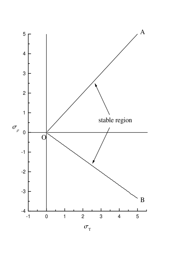
Figure 1: Region of stability in the $\sigma_{T}-\sigma_{\rho}$ plane in the absence of the magnetic field ($\alpha=0,D=0$).

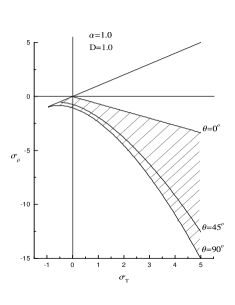
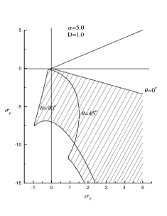
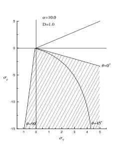
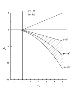
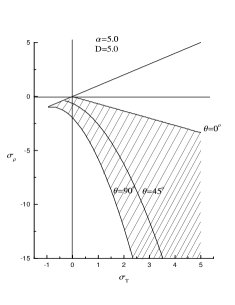
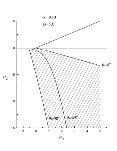
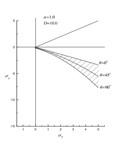
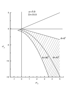
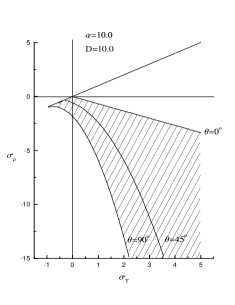
Figure 2: Regions of stability in the $\sigma_{T}-\sigma_{\rho}$ plane for presence of magnetic field including ambipolar diffusion ($\alpha\neq 0,D\neq 0$) for three values of $\theta$. The shaded areas are semi-stable regions where a disc-like clump can be formed.

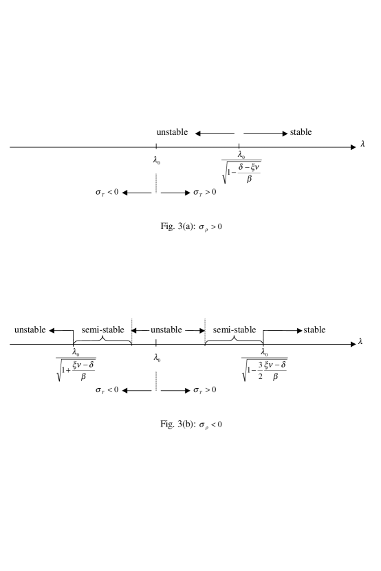
Figure 3: Different cases of stability, unstability, and semi-stability of the $\sigma_{T}-\sigma_{\rho}$ plane in terms of $\lambda$, wavelength of perturbation. Semi-stable regions of figure (b) depend on the magnetic field ($\alpha$) and the ambipolar diffusion strength (D).

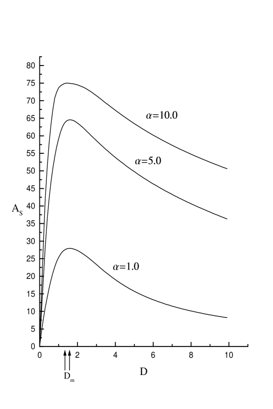
Figure 4: The area of semi-stable region, as a function of $D$ for three typical values of $\alpha$. Maximum of semi-stable region is occurred at a typical $D_{m}$.

References

- [1] Arons J., Max C.E., 1975, ApJ, 196, L77
- [2] Balbus S.A., 1986, ApJ, 303, L79
- [3] Balbus S.A., 1991, ApJ, 372, 25
- [4] Burkert A., Lin D.N.C., 2000, ApJ, 537, 270
- [5] Draine B.T., 1986, MNRAS, 220, 133
- [6] Falgarone E., Puget J.L., Pérault C.K., 1992, A&A, 257, 715
- [7] Field G.B., 1965,ApJ, 142, 531
- [8] Field G.B., Goldsmith D.W., Habing H.J., 1969, ApJ, 155, L49
- [9] Flannery B.P., Press W.H., 1979, ApJ, 231, 688
- [10] Gammie C.F., Lin Y., Stone J.M., Ostriker E.C., 2003, ApJ, 592, 203
- [11] Gilden D.L., 1984, ApJ, 283, 679
- [12] Glassgold A.E., Langer W.D., 1974, ApJ, 193, 73
- [13] Goldsmith P.F., Langer W.D., 1978, ApJ, 222, 881
- [14] Gomez-Pelaez A.J., Moreno-Isertis F., 2002, ApJ, 569, 766
- [15] Langer W.D., Velusamy T., Kuiper T.B., Levin S., Olsen E., Migenes V., 1995, ApJ, 453, 293
- [16] Larson R.B., 1981, MNRAS, 194, 809
- [17] Nakano T., 1980, PASJ, 32, 405
- [18] Ryden B.S., 1996, ApJ, 471, 822
- [19] Scalo J.M., 1977, ApJ, 213, 705
- [20] Schwarz J., McCray R., Stein R., 1972, ApJ, 175, 673
- [21] Shu F., 1991, The Physics of Astrophysics. University Science Books, Vol II, p. 360
- [22] Solomon P.M., Rivolo A.R., Barrett J., Yahil A., 1987, ApJ, 319, 730