Detection of molecular hydrogen at z = 1.15 toward HE 0515–4414

A new molecular hydrogen cloud is found in the sub-damped Ly$\alpha$ absorber [$\log N$(H i) = $19.88\pm 0.05$] at the redshift $z_{\rm abs}\,$= 1.15 toward the bright quasar HE 0515–4414 ($z_{\rm em}\,$= 1.71). More than 30 absorption features in the Lyman band system of H₂ are identified in the UV spectrum of this quasar obtained with the Space Telescope Imaging Spectrograph (STIS) aboard the Hubble Space Telescope. The H₂-bearing cloud shows a total H₂ column density $N$(H₂) $=(8.7^{+8.7}_{-4.0})\times 10^{16}$ cm${}^{-2}\,$  and a fractional molecular abundance $f_{{\rm H}_{2}}=(2.3^{+2.3}_{-1.1})\times 10^{-3}$ derived from the H₂ lines arising from the $J=0-5$ rotational levels of the ground electronic vibrational state. The estimated rate of photodissociation at the cloud edge $I_{0}\;\raise 1.29167pt\hbox{$<$\kern-7.5pt\raise-4.73611pt\hbox{$\sim$}}\;1.8\times 10^{-8}$ s^-1 is much higher than the mean Galactic disk value, $I_{\rm MW}\sim 5.5\times 10^{-11}$ s^-1. This may indicate an enhanced star-formation activity in the $z=1.15$ system as compared with molecular clouds at $z\sim 3$ where $I\sim I_{\rm MW}$. We also find a tentative evidence that the formation rate coefficient of H₂ upon grain surfaces at $z=1.15$ is a factor of 10 larger than a canonical Milky Way value, $R_{\rm MW}\approx 3\times 10^{-17}$ cm³ s^-1. The relative dust-to-gas ratio estimated from the [Cr/Zn] ratio is equal to $\tilde{k}=0.89\pm 0.19$ (in units of the mean Galactic disk value), which is in good agreement with a high molecular fraction in this system. The estimated line-of-sight size of $L\sim 0.25$ pc may imply that the H₂ is confined within small and dense filaments embedded in a more rarefied gas giving rise to the $z=1.15$ sub-damped Ly$\alpha$ absorber.

1 Introduction

The most abundant interstellar molecule in the universe, H₂, is currently observed not only in the Milky Way disk (e.g., Rachford et al. 2002) and halo (e.g., Richter et al. 2003a), but also in the Magellanic Clouds (e.g., Tumlinson et al. 2002) and in more distant regions of the universe such as intervening damped Ly$\alpha$ absorbers (DLAs) seen in spectra of background quasars (QSOs). The DLAs are the systems with neutral hydrogen column densities $N$(H i) $>2\times 10^{20}$ cm${}^{-2}\,$. They are believed to originate in protogalactic disks (Wolfe et al. 1995). The systems with lower hydrogen column densities, $10^{19}$ cm${}^{-2}\,$  $\;\raise 1.29167pt\hbox{$<$\kern-7.5pt\raise-4.73611pt\hbox{$\sim$}}\;N$(H i) $\leq 2\times 10^{20}$ cm${}^{-2}\,$, are formally called sub-DLAs. The sub-DLAs may also be related to intervening galaxies. At the moment there are known 9 molecular hydrogen systems detected in DLAs and sub-DLAs in the redshift range from $z_{\rm abs}\,$= 1.96 to 3.39 (see Table 1).

In this paper, we present results from the analysis of a new 10th H₂ system detected at $z_{\rm abs}\,$= 1.15 in the sub-DLA toward the bright quasar HE 0515–4414. This is the first detection of H₂ with the STIS/HST at an intermediate redshift – a cosmological epoch when an enhanced star formation rate (SFR) is observed in young galaxies. The SFR shows a peak at $z\sim 1$ over the redshift interval $0\leq z\;\raise 1.29167pt\hbox{$<$\kern-7.5pt\raise-4.73611pt\hbox{$\sim$}}\;3$ (see, e.g., Hippelein et al. 2003 and references therein).

Molecular hydrogen, being an important coolant for gravitational collapse of gas clouds at $T\sim 10^{3}$ K, is known to play a central role in star formation processes, and thus one may expect that the SFR and the fractional abundance of H₂ are correlated. Studying H₂-bearing cosmological clouds leads to better understanding of the physical environments out of which first stellar populations were formed.

Table 1: Molecular hydrogen abundances and dust contents $\tilde{k}$ in cosmological H₂-bearing clouds

QSO	$z_{\rm abs}\,$	$\log N$(H i)		$\log N$(H2)	$\log f_{{\rm H}_{2}}$	$\tilde{k}^{\ast}$	H2 detection
$0515-4414$	1.151	19.88$\pm$	0.05	$16.94^{+0.23}_{-0.41}$	$-2.64^{+0.30}_{-0.27}$	$0.89\pm 0.19$	this paper
$0551-366$	1.962	20.50$\pm$	0.08	$17.42^{+0.63}_{-0.90}$	$-2.78^{+0.64}_{-0.90}$	$2.12\pm 0.48$	Ledoux et al. 2002
$0013-004^{a}$	1.973	20.70$\pm$	0.05	$19.84^{+0.10}_{-0.10}$	$-0.66^{+0.10}_{-0.10}$	$0.52\pm 0.10$	Ge & Bechtold 1997
$1444+014$	2.087	20.07$\pm$	0.07	$18.30^{+0.37}_{-0.37}$	$-1.48^{+0.38}_{-0.38}$	$0.77\pm 0.30$	Ledoux et al. 2003
$1232+082$	2.338	20.90$\pm$	0.10b	$\geq 17.19^{c}$	$\geq-3.41^{c}$	$0.35\pm 0.12$	Ge et al. 2001
$0841+129$	2.374	20.95$\pm$	0.10c	$14.56^{\dagger}$	$<-5.98$	$0.024\pm 0.005$	Petitjean et al. 2000
$0405-443$	2.595	20.90$\pm$	0.10	$18.16^{+0.21}_{-0.06}$	$-2.44^{+0.23}_{-0.12}$	$0.17\pm 0.06$	Ledoux et al. 2003
$0528-250$	2.811	21.35$\pm$	0.10d,e	${}^{c}18.22^{+0.23}_{-0.16}$	${}^{c}-2.83^{+0.25}_{-0.19}$	$0.29\pm 0.08$	Levshakov & Varshalovich 1985
$0347-3819$	3.025	20.63$\pm$	0.01	$14.61^{+0.02}_{-0.02}$	$-5.71^{+0.02}_{-0.02}$	$0.068\pm 0.013$	Levshakov et al. 2002
$0000-2620$	3.390	21.41$\pm$	0.08f	${}^{g}13.94^{\dagger}$	$\simeq-7.2$	$\leq 0.002$	Levshakov et al. 2000
Note: Column densities $N$(H i) and $N$(H2) are given in cm${}^{-2}\,$; †tentative H2 identification; ∗photospheric solar
abundances for Cr and Zn are taken from Grevesse & Sauval (1998), for Mg and Fe from Holweger (2001),
see Eq.(3).
aHigh resolution UVES data reveal a few H2 subcomponents spread over $\sim 700$ km s${}^{-1}\,$(Petitjean et al. 2002);
bSrianand et al. 2000; cLedoux et al. 2003; dLevshakov & Foltz 1988: eM$\o$ller & Warren 1993;
fProchaska & Wolfe 1999; gLevshakov et al. 2001.

Figure 1: Typical example for a relative wavelength shift between successive orders. The H₂ L2-0 P(3) line shows a difference of $\Delta\lambda\sim 0.04$ Å  ($\Delta v\sim 5$ km s${}^{-1}\,$). The lines at the bottom indicate the noise level.

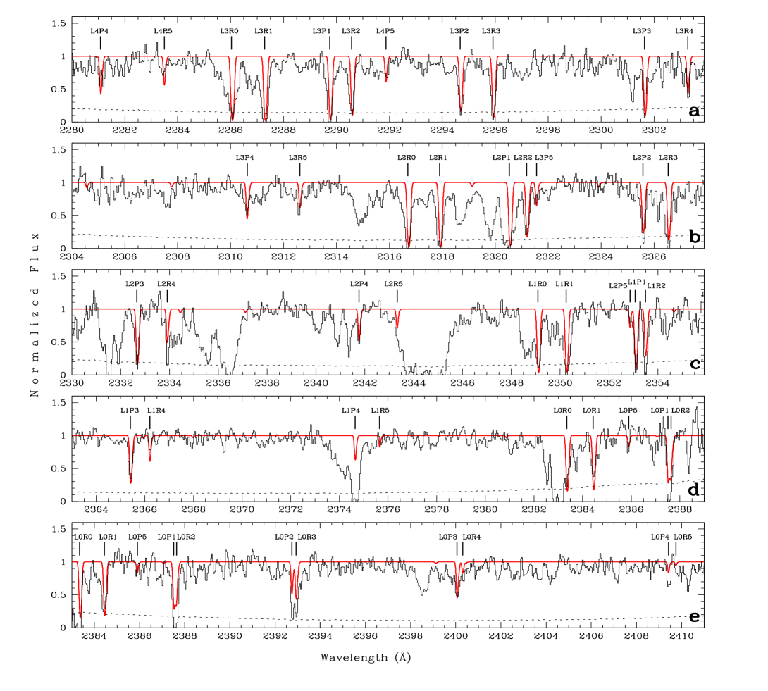
Figure 2: Continuum-normalized STIS spectra (histograms) of the quasar HE 0515–4414 (individual echelle orders marked by a, b, c, d, and e) and over-plotted synthetic H₂ profiles (smooth lines) arising from the rotational levels $J=0$ to $J=5$ of the lowest vibrational level $v=0$ in the ground electronic state $X^{1}\Sigma^{+}_{g}$. The noise level is shown by the dashed lines in each panel. The identified H₂ lines are calculated for a two-component model with the components located at the measured redshifts of the C i lines $z_{1}=1.15079$ and $z_{2}=1.15085$, having the widths $b_{1}=2.0$ km s${}^{-1}\,$, $b_{2}=3.5$ km s${}^{-1}\,$  (Quast et al. 2002), and a column density ratio $N_{2}/N_{1}=0.1$.

2 Observations

Spectral data of the quasar HE 0515–4414 ($z_{\rm em}\,$= 1.71, $V=14.9$; Reimers et al. 1998) in the UV range were obtained with the HST/STIS (Reimers et al. 2001). The medium resolution NUV echelle mode (E230M) and a $0.2^{\prime\prime}\times 0.2^{\prime\prime}$ aperture provides a resolution power of $\lambda/\Delta\lambda\sim 30,000$ (FWHM $\simeq 10$ km s${}^{-1}\,$). The overall exposure time was 31,500 s. The spectrum covers the range between 2279 Å  and 3080 Å  where the signal-to-noise ratio (S/N) per resolution element varies from S/N $\sim 20$ to $\sim 5$. The data reduction was performed by the HST pipeline completed by an additional inter-order background correction and by coadding the separate sub-exposures.

The spectral portion where the H₂ lines occur suffers from a poor S/N ratio ($\;\raise 1.29167pt\hbox{$<$\kern-7.5pt\raise-4.73611pt\hbox{$\sim$}}\;20$). An additional problem arises from the limited wavelength accuracy. The MAMA detectors produce an absolute wavelength definition between 0.5-1.0 pixel ($2\sigma$ limit as given by Brown et al. 2002). For our data 1 pixel corresponds to 0.038 Å. The spectral overlap of successive echelle orders allows to examine the wavelength errors from order to order. Using well-defined line profiles we find relative wavelength shifts of 0.02-0.05 Å  (see Fig. 1 for an example).

Additional echelle spectra of HE 0515–4414 were obtained during ten nights between October 7, 2000 and January 2, 2001 using the UV-Visual Echelle Spectrograph (UVES) installed at the VLT/Kueyen telescope. These observations were carried out under good seeing conditions (0.47–0.70 arcsec) and a slit width of 0.8 arcsec giving the spectral resolution of $\lambda/\Delta\lambda\sim 55,000$ (FWHM $\simeq 6$ km s${}^{-1}\,$). The VLT/UVES data have a very high S/N ratio ($\simeq$ 50–100 per resolution element) which allows us to detect weak absorption features.

The high resolution VLT/UVES data reveal two narrow components in the fine-structure C i lines associated with the sub-DLA at $z_{\rm abs}\,$= 1.15 (de la Varga et al. 2000). The stronger component at $z_{\rm abs}\,$= 1.15079 is separated from the weaker one by $\Delta v\simeq 8$ km s${}^{-1}\,$, and shows 2.8 times higher column density (Quast et al. 2002, hereafter QBR). Exactly at the redshift of C i lines we identified more than 30 absorption features in the Lyman band system of molecular hydrogen H₂.

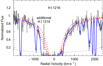
Figure 3: Part of the H i Ly$\alpha$ forest showing the damped Ly$\alpha$ system. The thin solid and dashed lines indicate the continuum normalized flux and the noise level, respectively. The thick solid curve represents the optimised Voigt profile model of the spectrum. The thick dashed curves show the individual profiles of the damped Ly $\alpha$ line corresponding to 70, 100, and 130 percent of the optimised column density $N$(H i) $=7.6\times 10^{19}$ cm${}^{-2}\,$. The blue part of the damped line overlaps with some additional H i absorption components clearly identified by the presence of many associated metal lines (Quast et al. 2003). The zero point of the radial velocity corresponds to the redshift $z=1.1508$.

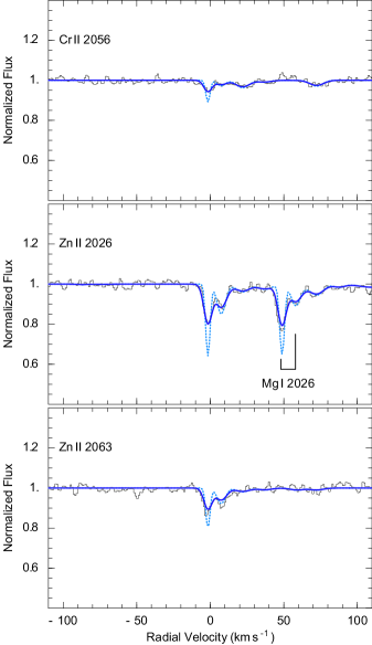
Figure 4: Parts of the UVES observations showing absorption arising from the ions Cr ii and Zn ii (histograms). The solid and dashed lines represent our optimised model and its deconvolution, respectively. Mg i $\lambda 2026$ absorption from the same sub-DLA is indicated. The zero point of the radial velocity corresponds to the redshift $z=1.1508$.

3 Measurements

In this section we describe the measurements of the neutral hydrogen column density, metal and dust content and the H₂ abundances in the $z_{\rm abs}\,$= 1.15 sub-DLA. These values are well known to be physically related. The formation and maintenance of diffuse H₂ in the Milky Way clouds is tightly correlated to the amount of interstellar dust grains, which provide the most efficient H₂ formation on their surfaces (see, e.g., Pirronello et al. 2000 and references therein).

3.1 Atomic hydrogen column density and metal abundance

In order to estimate the column density of atomic hydrogen contained in the sub-DLA, particular care has to be taken. Since the Doppler core of the Ly$\alpha$ line is completely saturated, only the Lorentzian part gives information about the line profile (Fig. 3). Moreover, the Lorentzian part is less pronounced than for typical DLAs and hence less distinguishable from the quasar continuum. Therefore, we simultaneously optimised the continuum and fitted the spectral features using standard Voigt profile fitting technique. The continuum is modelled as a linear function, and the Voigt function is calculated using the pseudo-Voigt approximation (Thompson et al. 1987).

Our optimized model (Fig. 3) reveals some additional absorption in the blue part of the damped Ly$\alpha$ line at $\Delta v\simeq-420$ km s${}^{-1}\,$. This additional absorption is H i Ly$\alpha$ which is seen also in metal lines. The whole sub-DLA system is spread over 700 km s${}^{-1}\,$  (Quast et al. 2003). This line together with other narrow absorption lines seen in the wings of the damped Ly$\alpha$ were included in the Voigt fitting.

The derived column density of atomic hydrogen in the sub-DLA is $\log N$(H i) $=19.88\pm 0.05$, where we estimated the standard deviation by varying the column density until the resulting model profile is apparently inconsistent with the observed data (Fig. 3).

To measure the metal abundance in the main sub-component of the $z_{\rm abs}\,$= 1.15 system we used the Zn ii $\lambda\lambda 2026,2063$ lines (Fig. 4). The presence of dust grains in DLAs is usually estimated from the abundance ratio [Cr/Zn] assuming that Zn is undepleted (Pettini et al. 1994). In our high S/N spectrum, only a weak Cr ii $\lambda 2056$ line was detected at $\Delta v=0$ km s${}^{-1}\,$  (Fig. 4). Other Cr ii lines ($\lambda\lambda 2062,2066$) are too weak to be visible. Their oscillator strengths scale as $f_{2056}:f_{2062}:f_{2066}=1:0.74:0.50$ (Bergeson & Lawler 1993).

Table 2: The H₂ column densities for different rotational levels from the $z_{\rm abs}\,$= 1.15 sub-DLA toward HE 0515–4414

Level	$\log N(J)$	$\log N(J)$	$\log N(J)$
	accepted	min	max
$J=0$	16.47	16.00	16.70
$J=1$	16.60	16.00	16.85
$J=2$	15.85	15.70	15.95
$J=3$	16.00	15.90	16.18
$J=4$	15.00	14.85	15.30
$J=5$	14.48	14.30	14.60

The column densities for Zn ii and Cr ii were calculated by Quast et al. (2003): $\log N$(Cr ii) = $12.01\pm 0.09$ and $\log N$(Zn ii) = $11.99\pm 0.02$. We used these values to estimate the dust-to-gas ratio in Sect. 4.2.

3.2 H₂ column densities

Molecular hydrogen at $z_{\rm abs}\,$= 1.15079 is detected in the $J=0$ up to $J=5$ rotational levels. At a spectral resolution of $\sim 10$ km s${}^{-1}\,$  it is not possible to resolve the internal structure in the H₂ lines observed in the C i absorption (see Fig. 1 in QBR). The H₂-bearing gas may also be distributed over a wider velocity range as compared with C i which is easily ionised by UV photons in optically thin zones. However, for a good approximation one can assume that H₂ traces, in general, the volume distribution of C i since such correlation is indeed observed in the Milky Way (e.g., Federman et al. 1980). Therefore, in our H₂ analysis we used a two-component model based on the observations of C i by QBR. We note that the C i data were obtained with higher spectral resolution (FWHM $\simeq 5.5$ km s${}^{-1}\,$) and considerably higher signal-to-noise ratio (up to S/N $\simeq 130$ for the parts of the spectrum with C i lines).

Panels a – e in Fig. 2 present echelle orders of the STIS spectra of HE 0515–4414 (histograms) in the wavelength regions of the H₂ Lyman 0-0 to 4-0 bands, together with a two-component Voigt profile fit of the data (smooth lines). It is seen that some of the identified H₂ transitions are contaminated by the Ly$\alpha$ forest or blended with metals from different intervening systems. This hampers significantly the measurements of accurate equivalent widths and their analysis through the curve of growth. Moreover, the noise level (shown by the dashed line) is rather high for the available STIS data and this may explain why some of H₂ features are inconsistent with others. For instance, the observational profile of L4P4 in panel a differs from those of L3R4 (a), L3P4 (b), L2R4 and L2P4 (c), and L1R4 (d). Relative strengths of the L0R0 and L0R1 lines from different echelle orders (panels d and e) are not consistent (L0R0 is partly blended with Fe ii $\lambda 2383$ at $z=0$). The apparent depths of the close pairs L0P2 + L0R3 (e) and L0P1 + L0R2 (e and d), as well as the single lines L1R2, L2R4 (c) are deeper than those calculated from the simultaneous fit to all H₂ lines.

Under these circumstances a standard $\chi$-square fitting cannot provide a statistically valuable measure of goodness-of-fit. To estimate model parameters we required that the calculated spectra were within 1 $\sigma$ uncertainty range for the majority of the unblended H₂ profiles or their unblended portions which match the data.

We tried to optimize a set of the H₂ column densities for the two-component model with the components located at the measured redshifts of the C i lines $z_{1}=1.15079$ and $z_{2}=1.15085$. The broadening $b$-parameters were fixed at $b_{1}=2.0$ km s${}^{-1}\,$, $b_{2}=3.5$ km s${}^{-1}\,$  (as deduced from the C i lines by QBR), but a column density ratio between the sub-components, $N_{2}/N_{1}$, was a free parameter ranging from 0.03 to 0.36 (the latter corresponds to the C i column density ratio found in QBR).

For a given H₂ component, the same $b$-parameter was used independently of the rotational level. The column density in each $J$ level was derived from several calculations of the Voigt profiles with a fixed value of $N_{2}/N_{1}$ and different $N(J)$ which match the observational spectra. The limiting values of $N(J)$ (an adjustable minimum and maximum) were chosen to estimate the uncertainty interval for column densities.

All identified transitions from $J=0$ and 1 are optically thick, but the apparent central intensities of the L0R0 and L0R1 lines (d) are not zero (we consider the L0R0 line in panel e as corrupted by a bad merging of different spectra). These lines restrict $N(0)$ and $N(1)$ by, respectively, $5\times 10^{16}$ and $7\times 10^{16}$ cm${}^{-2}\,$  at $N_{2}/N_{1}=0.03$. On the other hand, we observe neutral carbon which is usually shielded in molecular clouds from the background ionising UV radiation by the H₂ absorption arising from the $J=0$ and 1 levels. An essential shielding in H₂ lines occurs when $N$(H₂) $\;\raise 1.29167pt\hbox{$>$\kern-7.5pt\raise-4.73611pt\hbox{$\sim$}}\;10^{16}$ cm${}^{-2}\,$. This gives us a hint at a possible range of $N(J=0,1)$.

For the lower value of $N_{2}/N_{1}=0.03$, the contribution from the second H₂ component is negligible, but the synthetic profiles are systematically narrower as compared with the data. The presence of the second component is, therefore, important. On the other hand, the maximum value of $N_{2}/N_{1}=0.36$ provides too wide synthetic profiles even with $N(0)=N(1)=10^{16}$ cm${}^{-2}\,$. We found that with $N_{2}/N_{1}\sim 0.1$ an optimal set of the H₂ column densities may be deduced. An example of such solution is shown in Fig. 2. The obtained results are given in Table 2.

4 Discussion

We investigate now the physical conditions in the $z_{\rm abs}\,$= 1.15 H₂-bearing cloud by considering the processes and parameters that balance the formation and dissociation of molecular hydrogen. Since our observations show a relatively high metallicity in this sub-DLA, [Zn/H] = $-0.49\pm 0.10$ [i.e., $Z\sim\bigl{(}\frac{1}{4}$ - $\frac{2}{5}\bigr{)}Z_{\odot}$], and the dust content is approximately similar to the mean value for the cold gas in the Galactic disk ($\tilde{k}\sim 0.9$), we consider catalytic reactions on the surfaces of dust grains (Hollenbach & Salpeter 1971) as the dominant H₂ formation process, whereas ion-molecular gas phase reactions (Black 1978) are less efficient.

The measured column densities can be used to estimate the kinetic temperature, $T_{\rm kin}$, the gas density, $n_{\rm H}$, the photodissociation rate, $I$, and the rate of molecular formation on grains, $R$. However, in view of the large uncertainties in the column densities $N$(0) and $N$(1), we can only provide an order-of-magnitude estimate for these parameters.

Another obstacle in the H₂ analysis is that the balance equation is related to the space densities of H i and H₂. In case of homogeneous clouds one can assume that $n$(H i)/$n$(H₂) $\approx N$(H i)/$N$(H₂). However, this assumption may not be correct for DLAs where multiphase structures and complex profiles are usually observed. Observations show that with each step in increasing spectral resolution the profiles break up into subcomponents down to the new resolution limit.

The sub-DLA at $z_{\rm abs}\,$= 1.15 reveals, for example, transitions from neutrals and low ions (as C i, O i, C ii, Si ii) to highly ionized ions (as C iv, Si iv) spread over $\Delta v\simeq 700$ km s${}^{-1}\,$  (Quast et al. 2003) which implies that the neutral H₂-bearing cloud(s) is embedded in a lower density, higher temperature gas. Neutral hydrogen H i can be spread over all gas phases that contain neutral gas with and without molecules. The H₂ on the other hand may have a very inhomogeneous distribution in DLAs and concentrate in small clumps (Hirashita et al. 2003). Thus, only a fraction of the total H i may be relevant to the formation of H₂. In our Galaxy, for instance, ‘tiny-scale atomic structures’ (TSAS) and ‘small-area molecular structures ’ (SAMS) in the ISM are observed (e.g., Lauroesch & Meyer 1999; Heithausen 2002). They show very high densities ($n_{\rm H}\sim 10^{3}-10^{5}$ cm${}^{-3}\,$) and very small sizes ($L\sim$ a few AU).

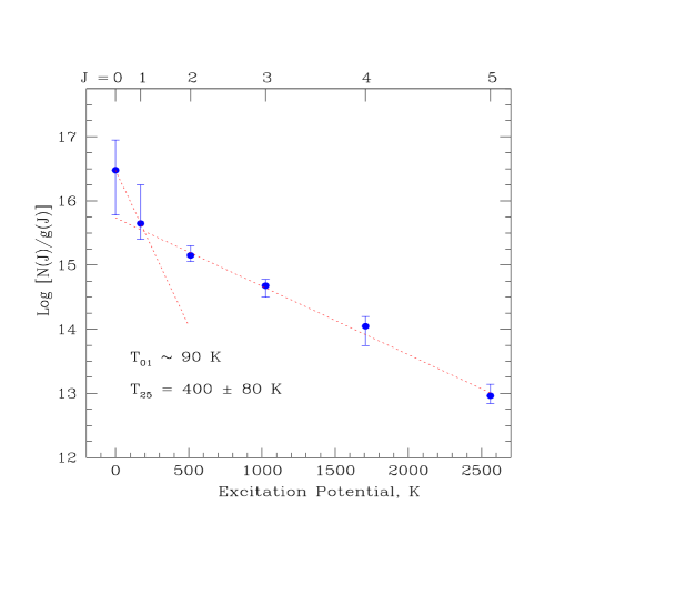
Figure 5: H₂ rotational excitation in the $z_{\rm abs}\,$= 1.15 sub-DLA toward HE 0515–4414. The logarithmic column densities $N(J)$, divided by the statistical weight $g(J)$ for each state $J$, are plotted against the excitation potential. The dashed lines represent fits from a theoretical Boltzmann distribution. The rotational ground states, $J=0$ and 1, fit on a line that is defined by a temperature of $T_{01}=90$ K. The excited levels, $J=2-5$, fit on a line with $T_{25}=400\pm 80$ K, possibly indicating excitation mechanisms through UV pumping and H₂ formation pumping.

To take this uncertainty into account, a scaling factor $\phi\leq 1$ for the H i column density can be introduced. Following Richter et al. (2003b), who observed similar complex structures in the Milky Way halo molecular clouds, we define

$$\left[\frac{n({\rm H\,\scriptstyle\rm I})}{n({\rm H}_{2})}\right]_{c}=\phi\,\frac{N({\rm H\,\scriptstyle\rm I})}{N({\rm H}_{2})}\;,$$ (1)

where $c$ stands for the cloudlet(s) where H₂ is confined and $N$(H i) is the total neutral hydrogen column density along the sightline within the absorber.

4.1 Kinetic temperature

The kinetic temperature of the gas is usually estimated through the excitation temperature $T_{01}$ describing the relative populations of the $J=0$ and $J=1$ levels. This temperature is proportional to the negative inverse of the slope of the excitation diagram drawn through the points of the respective $J$ levels in a plot $\log[N(J)/g(J)]$ versus $E(J)$ shown in Fig. 5. Here, $E(J)$ is the excitation energy of the rotational level $J$ relative to $J=0$, and $g(J)$ is its statistical weight.

Figure 5 shows that the value of $T_{01}$ is rather uncertain in our case because of large errors in $N(0)$ and $N(1)$. Its mean value $T_{01}\simeq 90$ K corresponds to the excitation diagram shown by the dotted line, and its upper limit is about 270 K, which represents, probably, an upper limit for $T_{\rm kin}$  of the gas in the main sub-component of the $z_{\rm abs}\,$= 1.15 system.

For levels with $J=2,3,4$, and 5 the accuracy of the column densities is higher and we find $T_{25}=400\pm 80$ K. The difference between $(T_{01})_{\rm max}$ and $(T_{25})_{\rm min}$ is not significant and the points in Fig. 5 can be fitted, in principle, to a single excitation diagram. But the previous analysis of the fine-structure level populations of C i, where the most probable value for $T_{\rm kin}$  of 240 K was found (QBR), indicates that these two temperatures may not be equal. This is also in line with results on the H₂ study in the Milky Way which revealed that single excitation diagrams fit usually only optically thin lines with $N$(H₂) $<10^{15}$ cm${}^{-2}\,$  (Spitzer & Cochran 1973). For higher column densities, there is ‘bifurcation to two temperatures, depending on the $J$ levels’ (Jenkins & Peimbert 1997).

4.2 Fractional molecularization and dust content

According to our calculations presented in Sect. 3.1, the total H i column density in the main sub-component is $N$(H i) $=(7.6\pm 0.9)\times 10^{19}$ cm${}^{-2}\,$. With $N$(H₂) $=(8.7^{+8.7}_{-4.0})\times 10^{16}$ cm${}^{-2}\,$, the ratio of H nuclei in molecules to the total H nuclei is

$$f_{{\rm H}_{2}}=\frac{2N({\rm H}_{2})}{N({\rm H})}=(2.3^{+2.3}_{-1.1})\times 10^{-3}\;,$$ (2)

where $N$(H) = $N$(H i) + 2$N({\rm H}_{2})$.

Listed in Table 1 are the molecular hydrogen fractions in all known H₂ systems. The $f_{{\rm H}_{2}}$ values were derived in the standard way assuming the scaling factor $\phi=1$. This may imply that the listed molecular hydrogen fractional abundances are systematically underestimated.

In Fig. 6 we compare these abundances with the dust-to-gas ratios, $\tilde{k}$, estimated from (Vladilo 1998):

$$\tilde{k}=\frac{10^{[{\rm X}/{\rm H}]_{\rm obs}}}{f_{\rm X,ISM}-f_{\rm Y,ISM}}\left(10^{[{\rm X}/{\rm Y}]_{\rm obs}}-1\right)\;,$$ (3)

where X and Y are two heavy elements with different depletions in dust. For all systems except Q 0405–443 and Q 1232+082 we used X = Zn ii and Y = Cr ii with their fractions in dust $f_{\rm Zn,ISM}=0.587\pm 0.048$ and $f_{\rm Cr,ISM}=0.920\pm 0.010$ referring to the Galactic interstellar medium (Vladilo 2002, hereafter V02). Since column densities for Zn ii and Cr ii are not known for Q 1232+082, we used in this case X = Mg ii, Y = Fe ii and $f_{\rm Mg,ISM}=0.715\pm 0.056$, $f_{\rm Fe,ISM}=0.939\pm 0.004$  from V02, although Mg and Fe may have not the same nucleosynthetic history. For Q 0405–443, the Cr ii abundance is not available and we used Fe ii instead of Cr ii. The errors of the $\tilde{k}$ values were calculated by applying error propagation method to the column density measurements quoted in the literature.

Figure 6 demonstrates an apparent correlation between $f_{{\rm H}_{2}}$ and $\tilde{k}$ in the range $0\leq\tilde{k}\leq 1$ which supports the assumption that molecular hydrogen abundances in quasar absorbers are governed by the dust content similar to that observed in the Galaxy. This conclusion rises the question: Why is the H₂ detection in QSO absorbers in this case so rare (lower than 30% according to Ledoux et al. 2003) ? Following Hirashita et al. (2003), we suppose that a relative paucity of H₂ observations in DLAs may be caused by a bias against finding H₂ in dense molecular clumps that have a small angular extent and thus a small volume filling factor. DLAs are mainly associated with diffuse clouds that have large volume filling factor and low molecular fractions, but they may also contain a small size dense filaments like the above mentioned TSAS or SAMS. Besides, low metallicity of the QSO absorbers can also significantly suppress H₂ formation (Liszt 2002).

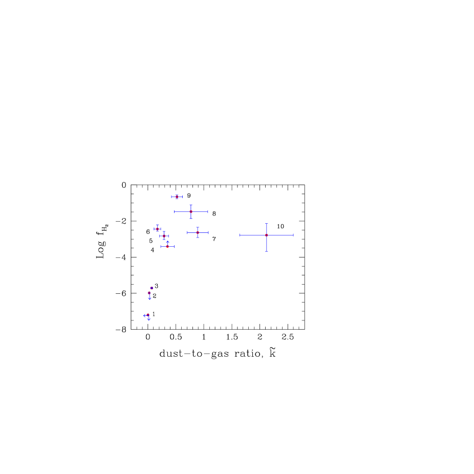
Figure 6: Relation between H₂ fractional abundance $f_{{\rm H}_{2}}$ plotted on a logarithmic scale and relative dust-to-gas ratio $\tilde{k}$ (with respect to the mean Milky Way value) in DLAs and sub-DLAs. Indicated by numbers are the systems found in spectra of QSOs 0000–2620 (1), 0841+129 (2), 0347–3819 (3), 1232+082 (4), 0528–250 (5), 0405–443 (6), 0515–4414 (7), 1444+014 (8), 0013–004 (9), and 0551–366 (10). A correlation between the two quantities in the range $0\leq\tilde{k}\leq 1$ is apparent (a large shift of $\tilde{k}$ for Q 0551–366 is probably caused by systematic errors in the data obtained by Ledoux et al. 2002, see text).

One point in Fig. 6 (Q 0551–366) shows an unrealistic high dust-to-gas ratio, about 2 times the Galactic value. This large value may be, probably, explained by systematic errors in the measurement of the Zn ii column density. For instance, the relative abundance of Si, [Si/H] $=-0.42\pm 0.11$, differs significantly from [Zn/H] $=-0.08\pm 0.12$ according to Ledoux et al. (2002). The fraction of these elements in dust in the Milky Way is approximately identical, $f_{\rm Si,ISM}=0.691\pm 0.069$ and $f_{\rm Zn,ISM}=0.587\pm 0.048$ (V02). At [Fe/H] $=-0.90\pm 0.11$, Ledoux et al. measured [Si/Fe] $\sim 0.5$ which is in line with other observations (see Fig. 1 in V02). This means that [Zn/H] is most likely overestimated in the $z_{\rm abs}\,$= 1.962 system.

4.3 H₂ formation and photodissociation rates

In equilibrium between formation on grains with rate coefficient $R$ (cm³ s^-1) and photodissociation with rate $I$ (s^-1), we may write that (Jura 1975b)

$$In_{{\rm H}_{2}}=Rnn_{\rm H}\approx 0.11\beta_{0}n_{{\rm H}_{2}}\>,$$ (4)

where $n=n_{\rm H}+2n_{{\rm H}_{2}}$, and $\beta_{0}$ is the photoabsorption rate depending on the local UV radiation field (one may neglect the $J$ dependence of $\beta$ for an optically thick cloud since the photoabsorption rates from the levels $J\geq 2$ are low).

To estimate the formation rate of H₂ upon grain surfaces $Rn_{\rm H}$, we use approximation described by Jura (1975b). It assumes that $(i)$ the levels $J=4$ and $J=5$ are populated by direct formation pumping and by UV pumping from $J=0$ and $J=1$, $(ii)$ the self-shielding in the levels $J=0$ and $J=1$ is about the same, $(iii)$ the upper levels $J=4$ and $J=5$ are depopulated by spontaneous emission (which is valid if $n_{\rm H}<10^{4}$ cm${}^{-3}\,$). We do not consider additional rotational excitation of H₂ caused by a shock because restrictions on the gas density ($n_{\rm H}\sim 100$ cm${}^{-3}\,$) and kinetic temperature ($T_{\rm kin}\leq 240$ K) set by the observations of C i, C i^∗, and C i^∗∗ (QBR) show that collisional excitation of the levels $J=4$ and $J=5$ is not significant. Using the cascade redistribution probabilities $p_{4,0}=0.26$ and $p_{5,1}=0.12$, calculated by Jura (1975a), and assuming $T_{\rm kin}=90$ K, we can re-write Eqs. (3a) and (3b) from Jura (1975b) in the form

$$[Rn_{\rm H}]_{c}=2.35\times 10^{-9}\frac{N(4)}{N({\rm H\,\scriptstyle\rm I})}\phi^{-1},$$ (5)

and

$$[Rn_{\rm H}]_{c}=9.15\times 10^{-9}\frac{N(5)}{N({\rm H\,\scriptstyle\rm I})}\phi^{-1}.$$ (6)

By substituting numerical values in (5) and (6) we obtain, respectively, $[Rn_{\rm H}]_{c}=(3.1^{+3.1}_{-1.0})\times 10^{-14}\phi^{-1}$ s^-1 and $(3.6\pm 1.2)\times 10^{-14}\phi^{-1}$ s^-1, which are consistent in the range $[Rn_{\rm H}]_{c}=(4.1\pm 1.7)\times 10^{-14}\phi^{-1}$ s^-1, and independent on the local value of $\beta_{0}$, as pointed out by Jura (1975b).

To estimate the photodissociation rate at the cloud surface $I_{0}$, the shielding effect is to be taken into account. The shielding factor, $S$, depends on line overlap, self-shielding of H₂, and continuum absorption. Lee et al. (1996) showed that these various factors can be well represented by the H₂ column density. They calculated the values of $S$ as a function of $N$(H₂) for a turbulent velocity of 3 km s${}^{-1}\,$, which suits well for our case. From their Table 10 we find $S=(1.928^{+1.075}_{-0.656})\times 10^{-3}$ for $N$(H₂) = $(8.7^{-4.0}_{+8.7})\times 10^{16}$ cm${}^{-2}\,$, respectively. This gives us a rough estimate of $I_{0}=Rn_{\rm H}N$(H i)$/SN$(H₂) $=1.8\times 10^{-8}$ s^-1 (with the uncertainty of about 120%), or $\beta_{0}\simeq 1.6\times 10^{-7}$ s^-1. The result obtained should be considered, however, as an upper limit on $\beta_{0}$ since in our estimations we assumed that the H₂ is one singe gas cloud. If, in reality, the H₂ is inhomogeneously distributed among several cloudlets, the value of $\beta_{0}$ should be lower.

In the Milky Way, the mean value for $\beta_{0,\rm halo}\approx 0.5\beta_{0,\rm disk}=2.5\times 10^{-10}$ s^-1 (e.g., Richter et al. 2003b) and, thus, we may conclude that the H₂ in the $z_{\rm abs}\,$= 1.15 sub-DLA is probably exposed to a radiation field with the intensity much higher than the mean Galactic value. For comparison, molecular clouds in the LMC and SMC also reveal 10-100 times more intense UV radiation field than the Galactic one (Browning et al. 2003). High rotational excitation of the H₂ observed in the LMC/SMC gas and at $z_{\rm abs}\,$= 1.15 is compared with Galactic data in Fig. 7. We note that the upper limit on the local UV field at $z_{\rm abs}\,$= 1.15 of about 100 times the Galactic value was independently determined from the analysis of the C i fine-structure lines by QBR.

We can also estimate the photodissociation rate produced by the intergalactic UV background (UVB) field on the surface of a cloud (Hirashita et al. 2003):

$$I_{\rm UVB}\sim 1.38\times 10^{-12}J_{21}\;,$$ (7)

where $J_{21}$ (in units $10^{-21}$ erg cm${}^{-2}\,$s^-1 Hz^-1 str^-1) is the UVB intensity at 1 Ryd averaged for all the solid angle. At $z_{\rm abs}\,$= 1.15, $J_{21}\simeq 0.4$ (Haardt & Madau 1996), and thus $I_{\rm UVB}$ is of the order of $5\times 10^{-13}$ s^-1, which is about 4 orders of magnitude lower as compared with the derived value of $I_{0}\;\raise 1.29167pt\hbox{$<$\kern-7.5pt\raise-4.73611pt\hbox{$\sim$}}\;10^{-8}$ s^-1. The presence of bright young stars in the $z_{\rm abs}\,$= 1.15 sub-DLA is therfore required to maintain this high value of $I_{0}$.

Star-formation activity is not, however, intense in the H₂-bearing clouds at higher redshift. For example, the UV radiation fields in the $z_{\rm abs}\,$= 3.025 H₂ absorber toward Q 0347–3819 and in the Galactic ISM are very much alike (Levshakov et al. 2002). Other examples may be found in Ledoux et al. (2003).

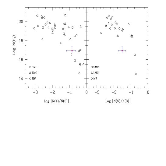
Figure 7: Total column density of H₂ vs. excitation ratios $N(4)/N(2)$ and $N(5)/N(3)$, for LMC, SMC, Milky Way (data are taken from Browning et al. 2003), and sub-DLA at $z_{\rm abs}\,$= 1.15 (dots with error bars). A systematically higher rotational excitation is observed in the Magellanic Clouds and in the sub-DLA as compared with Galactic data points.

4.4 Gas density and H₂ formation rate coefficient

We now consider constraints on the volumetric gas density $n_{\rm H}$ and the H₂ formation rate coefficient $R$ stemming from the foregoing estimation of $[Rn_{\rm H}]_{c}\sim 4\times 10^{-14}\phi^{-1}$ s^-1.

A useful reference point is provided by the $J=2$ level. The population of this level is more directly affected by collisional processes, since it has a longer radiative lifetime as compared with $J=3$ and other levels. The critical density, $n^{\rm cr}_{\rm H}$, at which the probability of collisional and radiative de-excitation of $J=2$ are equal is 200 cm${}^{-3}\,$, if $T_{\rm kin}$  = 100 K, and $n^{\rm cr}_{\rm H}=80$ cm${}^{-3}\,$, if $T_{\rm kin}$  = 240 K (the collisional de-excitation rate coefficients $q_{jj^{\prime}}$ are taken from Forrey et al. 1997). If $n_{\rm H}>n^{\rm cr}_{\rm H}$, collisional de-excitation becomes important.

To estimate $n_{\rm H}$, the grain formation rate of H₂ should be known or vice versa. $R$ is a complex function of the gas and dust temperature and other poorly known parameters (Hollenbach & McKee 1979). According to their calculations, $R_{\rm MW}\approx 3\times 10^{-17}$ cm³ s^-1. Using this value, we find $n_{\rm H}\;\raise 1.29167pt\hbox{$>$\kern-7.5pt\raise-4.73611pt\hbox{$\sim$}}\;1300$ cm${}^{-3}\,$, if $\phi\leq 1$. However, for such large density, the $J=0$ and $J=2$ levels as well as the $J=1$ and $J=3$ levels should be in thermal equilibrium, which we do not observe. Moreover, the upper limit on the gas density set from the excitation of C i is 110 cm${}^{-3}\,$  (QBR). If we tentatively adopt $n_{\rm H}\sim 100$ cm${}^{-3}\,$, then $R\sim 10R_{\rm MW}$.

This value of $R$ is larger than predicted in theoretical calculations, but it is conceivable that $R$ may vary in space since we observe considerable variations in the UV extinction among different clouds. A low grain formation rate of H₂ ($R\sim 0.1R_{\rm MW}$) was, for instance, recently estimated in the LMC and SMC by Browning et al. (2003). Although our high value of $R$ is consistent with the best determinations of upper limits to $R$ toward $\gamma$ Peg, $\nu$ Sco, $\lambda$ Sco etc. (Jura 1974), we cannot without further observations conclude that this result is certain. To test whether or not the grain formation rate coefficient $R$ exceeds the value of $R_{\rm MW}$, a higher accuracy for the $N$(0) and $N$(1) column densities is needed to verify that $T_{01}\neq T_{25}$.

For $n_{\rm H}\sim 100$ cm${}^{-3}\,$, the linear thickness of the H₂-bearing cloud is small, $L\sim 0.25$ pc. Similar characteristics of molecular hydrogen small structures are found in intermediate-velocity clouds (IVC) in the Milky Way halo (Richter et al. 2003b).

5 Conclusions

We have analyzed the HST/STIS and VLT/UVES spectra of the quasar HE 0515–4414 and deduced the physical properties of the H₂-bearing cloud embedded in the sub-DLA at $z_{\rm abs}\,$= 1.15. The main conclusions are as follows:

1. In the STIS spectrum of HE 0515–4414 we have identified over 30 absorption features with the Lyman lines arising from the $J=0-5$ rotational levels of the ground electronic vibrational state of H₂. These lines have exactly the same redshift as the fine-structure transitions in C i identified earlier by QBR in the UVES spectrum of this quasar.

2. We find a total H₂ column density of $N$(H₂) $=(8.7^{+8.7}_{-4.0})\times 10^{16}$ cm${}^{-2}\,$  and a molecular hydrogen fraction of $f_{{\rm H}_{2}}=(2.3^{+2.3}_{-1.1})\times 10^{-3}$.

3. From the measured ratios [Cr/H] $=-1.54\pm 0.11$ and [Zn/H] $=-0.49\pm 0.10$ we calculated the relative dust-to-gas ratio $\tilde{k}=0.89\pm 0.19$ (in units of the mean Galactic disk value) in the molecular cloud (the ratio [Cr/Zn] is usually used to indicate the presence of dust in DLAs). The derived H₂ fractional abundance correlates with the dust content showing increasing $f_{{\rm H}_{2}}$ with increasing $\tilde{k}$ in cosmological molecular clouds. This indicates that catalytic reactions on the surfaces of dust grains is the dominant H₂ formation process not only in the diffuse clouds in the Milky Way but in the DLA systems as well.

4. Two excitation temperatures are required to describe the rotational excitation of the H₂ gas: for the $J=0$ and $J=1$ levels we find $T_{01}\sim 90$ K and the upper limit for the kinetic temperature of the gas of about 270 K. For $J=2-5$ we derive $T_{25}=400\pm 80$ K.

5. From the relative populations of H₂ in the $J=4$ and 5 rotational levels we estimated the rate of photodissociation at the cloud surface $I_{0}\;\raise 1.29167pt\hbox{$<$\kern-7.5pt\raise-4.73611pt\hbox{$\sim$}}\;1.8\times 10^{-8}$ s^-1 which is much higher than the mean Galactic disk value. Star-formation activity may be very intense in the close vicinity of the H₂-bearing cloud, which is in line with the observed high SFR in galaxies at intermediate redshift, $z\sim 1$. At higher redshift, $z\sim 3$, we do not observe such intense UV fields in the molecular clouds.

6. We also find that the formation rate coefficient of H₂ upon grain surfaces is probably 10 times higher as compared with the conventional value adopted for the Milky Way, $R_{\rm MW}\approx 3\times 10^{-17}$ cm³ s^-1.

7. We find that in order to be consistent with the measurements of the population ratios of the fine-structure levels in C i, the gas density in the molecular cloud should be $\sim 100$ cm${}^{-3}\,$, which implies that the line-of-sight size of this cloud is small, $L\sim 0.25$ pc. Small sizes and a low level of the H₂ detections in the DLAs favour calculations of Hirashita et al. (2003) who showed that the H₂ may have very inhomogeneous distribution within these systems. The diffuse molecular hydrogen gas forms, probably, in small, dense filaments during the cooling and fragmentation phase in DLAs.

- (1) Abgrall, H., Roueff, E., Launay, F., Roncin, J.-Y., & Subtil, J.-L. 1993, A&AS, 101, 273
- (2) Bergeson, S. D., & Lawler, J. E. 1993, ApJ, 408, 382
- (3) Black, J. 1978, ApJ, 222, 125
- (4) Brown, T., Davies, J., Díaz-Miller, R. et al. 2002, in HST STIS Data Handbook, version 4.0, ed. B. Mobasher (Baltimore: STScI)
- (5) Browning, M. K., Tumlinson, J., & Shull, J. M. 2003, ApJ, 582, 810
- (6) de la Varga, A., Reimers, D., Tytler, D., Barlow, T., & Burles, S. 2000, A&A, 363, 69
- (7) Federman, S. R., Glassgold, A. E., Jenkins, E. B., & Shaya, E. J. 1980, ApJ, 242, 545
- (8) Forrey, R. C., Balakrishnan, N., & Dalgarno, A. 1997, ApJ, 489, 1000
- (9) Ge, J., Bechtold, J., & Kulkarni, V. P. 2001, ApJ, 547, L1
- (10) Ge, J., & Bechtold, J. 1997, ApJ, 477, L73
- (11) Grevesse, N., & Sauval, A. J. 1998, Space Sci. Rev., 85, 161
- (12) Haardt, F., & Madau, P. 1996, ApJ, 461, 20
- (13) Heithausen, A. 2002, A&A, 393, L41
- (14) Hippelein, H., Maier, C., Meisenheimer, K. et al. 2003, A&A, 402, 65
- (15) Hirashita, H., Ferrara, A., Wada, K., & Richter, P. 2003, MNRAS, 341, L18
- (16) Hollenbach, D. J., & McKee, C. F. 1979, ApJS, 41, 555
- (17) Hollenbach, D., & Salpeter, E. E. 1971, ApJ, 163, 155
- (18) Holweger, H. 2001, in Solar and Galactic Composition, ed. R. F. Wimmer-Schweingruber, AIP Conf. Proc., 598, 23
- (19) Jenkins, E. B., & Peimbert, A. 1997, ApJ, 477, 265
- (20) Jura, M. 1975a, ApJ, 197, 575
- (21) Jura, M. 1975b, ApJ, 197, 581
- (22) Jura, M. 1974, ApJ, 191, 375
- (23) Lauroesch, J. T., & Meyer, D. M. 1999, ApJ, 519, L181
- (24) Ledoux, C., Petitjean, P., & Srianand, R. 2003, MNRAS, submit. (astro-ph/0302582)
- (25) Ledoux, C., Srianand, R., & Petitjean, P. 2002, A&A, 396, 429
- (26) Lee, H.-H., Herbst, E., Pineau des Forêts, G., Roueff, E., & Le Bourlot, J. 1996, A&A, 311, 690
- (27) Levshakov, S. A., Dessauges-Zavadsky, M., D’Odorico, S., & Molaro, P. 2002, ApJ, 565, 696
- (28) Levshakov, S. A., Molaro, P., Centurión, M., D’Odorico, S., Bonifacio, P., & Vladilo, G. 2001, in Deep Fields, eds. S. Cristiani, A. Renzini and R. E. Williams (Springer-Verlag: Berlin, Heidelberg), 334
- (29) Levshakov, S. A., Molaro, P., Centurión, M., D’Odorico, S., Bonifacio, P., & Vladilo, G. 2000, A&A, 361, 803
- (30) Levshakov, S. A., & Foltz, C. B. 1988, Soviet Astron. Lett., 14, 467
- (31) Levshakov, S. A., & Varshalovich, D. A. 1985, MNRAS, 212, 517
- (32) Liszt, H. 2002, A&A, 389, 393
- (33) Mller, P., & Warren, S. J. 1993, A&A, 270, 43
- (34) Petitjean, P., Srianand, R., & Ledoux, C. 2002, MNRAS, 332, 383
- (35) Petitjean, P., Srianand, R., & Ledoux, C. 2000, A&A, 364, L26
- (36) Pettini, M., Smith, L. J., Hunstead, R. W., & King, D. L. 1994, ApJ, 426, 79
- (37) Pirronello, V., Biham, O., Manicò, G., Roser, J., & Vidali, G. 2000, in Molecular Hydrogen in Space, eds. F. Combes and G. Pineau des Forêts (Cambridge: Cambridge Univ. Press), 71
- (38) Prochaska, J. X., & Wolfe, A. 1999, ApJS, 121, 369
- (39) Quast, R., Reimers, D. & Baade, R. 2003, in preparation
- (40) Quast, R., Baade, R., & Reimers, D. 2002, A&A, 386, 796 [QBR]
- (41) Rachford, B. L., Snow, T. P., Tumlinson, J. et al. 2002, ApJ, 577, 221
- (42) Richter, P., Sembach, K. R., & Howk, J. C. 2003a, A&A, 405, 1013
- (43) Richter, P., Wakker, B. P., Savage, B. D., & Sembach, K. R. 2003b, ApJ, 586, 230
- (44) Reimers, D., Baade, R., Hagen, H.-J., & Lopez, S. 2001, A&A, 374, 871
- (45) Reimers, D., Hagen, H.-J., Rodriguez-Pascual, P., & Wisotzki, L. 1998, A&A, 334, 96
- (46) Savage, B. D., Bohlin, R. C., Drake, J. F., & Budich, W. 1977, ApJ, 216, 291
- (47) Spitzer, L., Jr., & Cochran, W. D. 1973, ApJ, 186, L23
- (48) Srianand, R., Ledoux, C., & Petitjean, P. 2000, Nature, 408, 931
- (49) Thompson, P., Cox, D. E. & Hastings, J. B. 1987, J. Appl. Chryst, 20, 79
- (50) Tumlinson, J., Shull, J. M., Rachford, B. L. et al. 2002, ApJ, 566, 857
- (51) Turner, J., Kirby-Docken, K., & Dalgarno, A. 1977, ApJS, 35, 281
- (52) Vladilo, G. 2002, A&A, 391, 407 [V02]
- (53) Vladilo, G. 1998, ApJ, 493, 583
- (54) Wolfe, A. M., Lanzetta, K. M., Foltz, C. B., & Chaffee, F. H. 1995, ApJ, 454, 698