The Red Giant Branch Luminosity Function Bump

We present observational estimates of the magnitude difference between the luminosity function red giant branch bump and the horizontal branch ($\Delta\mathrm{F555W}^{\mathrm{bump}}_{\mathrm{HB}}$), and of star counts in the bump region ($R_{\mathrm{bump}}$), for a sample of 54 Galactic globular clusters observed by the HST. The large sample of stars resolved in each cluster, and the high photometric accuracy of the data allowed us to detect the bump also in a number of metal poor clusters.

To reduce the photometric uncertainties, empirical values are compared with theoretical predictions obtained from a set of updated canonical stellar evolution models which have been transformed directly into the HST flight system. We found an overall qualitative agreement between theory and observations. Quantitative estimates of the confidence level are hampered by current uncertainties on the globular cluster metallicity scale, and by the strong dependence of $\Delta\mathrm{F555W}^{\mathrm{bump}}_{\mathrm{HB}}$ on the cluster metallicity. In case of the $R_{\mathrm{bump}}$ parameter, which is only weakly affected by the metallicity, we find a very good quantitative agreement between theoretical canonical models and observations. For our full cluster sample the average difference between predicted and observed $R_{\mathrm{bump}}$ values is practically negligible, and ranges from $-$0.002 to $-$0.028, depending on the employed metallicity scale. The observed dispersion around these values is entirely consistent with the observational errors on $R_{\mathrm{bump}}$. As a comparison, the value of $R_{\mathrm{bump}}$ predicted by theory in case of spurious bump detections due to Poisson noise in the stellar counts would be $\sim$0.10 smaller than the observed ones.

We have also tested the influence on the predicted $\Delta\mathrm{F555W}^{\mathrm{bump}}_{\mathrm{HB}}$ and $R_{\mathrm{bump}}$ values of an He-enriched component in the cluster stellar population, as recently suggested by D’Antona et al. (d02 (2002)). We find that, under reasonable assumptions concerning the size of this He-enriched population and the degree of enrichment, the predicted $\Delta\mathrm{F555W}^{\mathrm{bump}}_{\mathrm{HB}}$ and $R_{\mathrm{bump}}$ values are only marginally affected.

1 Introduction

Stellar evolution models supply fundamental tools which enable one to constrain the structure of the Milky Way, the properties of extragalactic stellar systems, and the early evolution of the universe. During the last few years the substantial increase in the spatial resolution provided by the Hubble Space Telescope (HST), as well as the advent of wide field imagers in ground-based telescopes provided homogeneous and accurate photometry for large samples of stars in Galactic Globular Clusters (GGCs). This has made possible a thorough comparison between theoretical models of low mass stars and observations, over a broad metallicity range. This kind of comparisons play a crucial role in modern stellar astrophysics, because they provide stringent tests for the accuracy of current stellar evolution models (Renzini & Fusi Pecci rfp88 (1988); Castellani 1999).

In this context, the Red Giant Branch (RGB) luminosity function (LF) of GGCs is an important tool to test the chemical stratification inside the stellar envelopes (Renzini & Fusi Pecci rfp88 (1988)). The most interesting feature of the RGB LF is the occurrence of a local maximum in the luminosity distribution of RGB stars, which appears as a bump in the differential LF, and as a change in the slope of the cumulative LF. According to Thomas (thomas (1967)) and Iben (iben (1968)) this feature is caused by the sudden increase of H-abundance left over by the surface convection upon reaching its maximum inward extension at the base of the RGB. When the advancing H-burning shell encounters this discontinuity, its efficiency is affected (sudden increase of the available fuel), causing a temporary drop of the surface luminosity. After some time the thermal equilibrium is restored and the surface luminosity starts to increase again. As a consequence, the stars cross the same luminosity interval three times, and this occurrence shows up as a characteristic peak in the differential LF of RGB stars. Moreover, since the H-profile before and after the discontinuity is different, the rate of advance of the H-burning shell changes when the discontinuity is crossed, thus causing a change in the slope of the cumulative LF.

The brightness of the RGB bump is therefore related to the location of this H-abundance discontinuity, in the sense that the deeper the chemical discontinuity is located, the fainter is the bump luminosity. A comparison between the predicted bump luminosity and the observations allows a direct check of how well theoretical models for RGB stars predict the extension of convective regions in the stellar envelope; following Fusi Pecci et al. (fp90 (1990)), the observed magnitude difference between the RGB bump and the HB at the RR Lyrae instability strip ($\Delta{V}^{\mathrm{bump}}_{\mathrm{HB}}$) is usually employed in order to test the theoretical predictions for the bump brightness. This quantity presents several advantages from the observational point of view (see Fusi Pecci et al. fp90 (1990), and Salaris et al. scw02 (2002)) and it is empirically well-defined because it does not depend on a previous knowledge of the cluster distance.

Dating back to its first detection in the LF of the GGC 47 Tuc by King, Da Costa & Demarque (king (1985)), the RGB bump has been the subject of several theoretical and observational investigations (Fusi Pecci et al. fp90 (1990), Cassisi & Salaris cs97 (1997), Alves & Sarajedini alves (1999), Ferraro et al. f99 (1999), Zoccali et al. z99 (1999), Bergbusch & Vandenberg bergbusch (2001), Salaris, Cassisi & Weiss scw02 (2002) and references therein). However, a sound quantitative comparison between theory and observations was hampered by the size of the observed stellar samples along the RGB, and by the heterogeneity of the datasets. This problem was even more severe for the most metal-poor GGCs, since the RGB evolutionary timescales is significantly shorter in metal-poor than in metal-rich stars. However, Zoccali et al. (1999, hereinafter Z99), using a homogeneous set of data collected with HST, firmly detected the RGB bump in a large sample of GGCs covering a wide metallicity range.

This is the sixth in a series of papers aimed at investigating the RGB bump in the LF of GGCs. On the basis of a detailed set of evolutionary models Cassisi & Salaris (cs97 (1997)) showed that the predicted $\Delta{V}^{\mathrm{bump}}_{\mathrm{HB}}$was in agreement with empirical estimates of GGCs with accurate spectroscopic measurements of heavy-element abundances. This finding was further strengthened by the evidence that the $\Delta{V}^{\mathrm{bump}}_{\mathrm{HB}}$ is only marginally affected by atomic diffusion (Cassisi, Degl’Innocenti & Salaris cds97 (1997)). A more detailed comparison was provided by Z99 who found that theory and observations do agree at the level of $\approx 0.1$ mag.

A different kind of analysis was performed by Bono et al. (bono (2001), hereinafter B01), who compared the theoretical evolutionary lifetimes during the crossing of the H-discontinuity with the star counts across the RGB bump, a quantity that is sensitive to possible extra-mixing processes below the formal convective boundary. B01 have shown that star counts in the bump region are sensitive to the size of the jump in the H-profile left over when the envelope starts to recede, after achieving its maximum inward extension. Deep mixing phenomena (prior to the bump stage) able to dredge up an appreciable amount of He would change the size of the H-abundance jump, thus modifying the star counts in the bump region. The $R_{\mathrm{bump}}$ parameter was defined as the ratio between the star counts in the bump region $\mathrm{V}_{\mathrm{bump}}\pm 0.4$ and the star counts in the normalization region $\mathrm{V}_{\mathrm{bump}}+0.5<\mathrm{V}_{\mathrm{bump}}<\mathrm{V}_{\mathrm{bump}}+1.5$. The reasons for this choice of the bump and the normalization regions are that the former should be large enough to include all bump stars, while the latter is required to normalize the total number of stars sampled in each cluster. The comparison between theory and observations performed by B01 disclosed that the occurrence of a substantial efficiency of non-canonical extra-mixing before the RGB bump could be excluded. On the basis of theoretical arguments, Cassisi, Salaris & Bono (csb02 (2002)) more recently suggested to use the shape of the LF bump as a complementary diagnostic of partial mixing processes at the base of the outer convective zone, since it is sensitive to the shape of the H-discontinuity.

The key differences between this investigation and Z99 are the following: i) we adopted the sample of GGCs presented by Piotto et al. (snapshot (2002)) and for 54 of them we detected the RGB bump. This sample is approximately 30% larger than the sample by Z99; ii) we adopted the more robust HST flight photometric system (without reddening corrections) instead of the Johnson de-reddened bands. This approach avoids deceptive errors in the estimate of the visual magnitudes of both RGB bump and HB. As a matter of fact, the calibration to the standard Johnson system (Dolphin dolphin (2000)) requires the knowledge of the reddening. Therefore, the accuracy of the equivalent Johnson magnitudes depends on the accuracy of the adopted cluster reddening (see Piotto et al. snapshot (2002)); iii) the uncertainties of current parameters have been estimated using the completeness curves and the photometric errors obtained from a large number of artificial star experiments (see §2); iv) the comparison between theory and observations is based on an updated theoretical framework.

The main aim of this investigation is to provide new homogeneous measurements of the RGB bump, and in turn of its brightness with respect to the HB, for a sizable sample of GGCs that cover a wide range in metallicity ($-2.2\leq\textrm{[Fe/H]}\leq-0.3$), and to compare these measurements with predictions based on a new set of evolutionary models.

In the next section we present the observational database, and we briefly discuss the procedures adopted for the reduction and the calibration of the data. In this section we also outline the approach adopted to estimate the $\Delta\mathrm{F555W}^{\mathrm{bump}}_{\mathrm{HB}}$ and the $R_{\rm bump}$ parameters. In §3, we present the new theoretical models adopted in this investigation, while in §4 we compare theory and observations. Conclusions and future developments are discussed in §5.

2 The cluster database

We exploited our large photometric database of 74 GGCs observed in the HST $B$ (F439W) and $V$ (F555W) bands with the WFPC2 (Piotto et al. snapshot (2002)) to measure the $\Delta\mathrm{F555W}^{\mathrm{bump}}_{\mathrm{HB}}$ and $R_{\mathrm{bump}}$ parameters, that are related to the position and extension of the RGB bump. The observations, pre-processing, photometric reduction, and calibration of the instrumental magnitudes to the HST flight system as well as the artificial star experiments performed to derive star count completeness are described in Piotto et al. (snapshot (2002)). All photometric data have been processed following the same steps: after the pre-processing, the instrumental photometry for each cluster was obtained with DAOPHOT II/ALLFRAME; the correction for the CTE effect and the calibration to the flight system was performed following the prescriptions by Dolphin (dolphin (2000)).

For each cluster we measured a number of stars that ranges from a few thousands in the less massive clusters, to $\approx 47,000$ in NGC 6388. This and the high internal photometric accuracy, (the typical photometric error at the bump and ZAHB level ranges from a few $10^{-3}$ to a few $10^{-2}$ mag) allowed us to detect the RGB bump even in metal-poor clusters.

Table 1: Data for the 54 GGCs in our sample. The 26 clusters with more than 85 stars in the RGB Bump area are marked with an asterisk.

Object	$[M/H]_{CG97}$	$[M/H]_{ZW84}$	$\mathrm{F555W}_{\mathrm{bump}}$	$\Delta\mathrm{F555W}^{\mathrm{bump}}_{\mathrm{HB}}$	$N_{B}$	$N_{N}$	$R_{\mathrm{bump}}$
(1)	(2)	(3)	(4)	(5)	(6)	(7)	(8)
ic4499	-1.06	-1.29	17.42$\;\pm\;$0.04	-0.34$\;\pm\;$0.08	20	62	0.323$\;\pm\;$0.083
n0104∗ (47 Tuc)	-0.56	-0.57	14.58$\;\pm\;$0.03	0.32$\;\pm\;$0.08	295	480	0.615$\;\pm\;$0.046
n0362∗	-0.94	-1.06	15.46$\;\pm\;$0.04	-0.05$\;\pm\;$0.10	129	268	0.481$\;\pm\;$0.052
n1261	-0.89	-1.10	16.76$\;\pm\;$0.04	-0.09$\;\pm\;$0.08	70	172	0.407$\;\pm\;$0.058
n1851∗	-0.93	-1.15	16.12$\;\pm\;$0.04	-0.04$\;\pm\;$0.10	147	320	0.459$\;\pm\;$0.046
n1904 (M 79)	-1.16	-1.48	16.00$\;\pm\;$0.08	-0.26$\;\pm\;$0.11	69	130	0.531$\;\pm\;$0.079
n2808∗	-0.94	-1.16	16.29$\;\pm\;$0.03	-0.07$\;\pm\;$0.08	387	818	0.473$\;\pm\;$0.029
n4590 (M 68)	-1.78	-1.88	15.28$\;\pm\;$0.04	-0.45$\;\pm\;$0.09	29	38	0.763$\;\pm\;$0.188
n4833	-1.37	-1.65	15.21$\;\pm\;$0.03	-0.49$\;\pm\;$0.08	27	67	0.403$\;\pm\;$0.092
n5024∗ (M 53)	-1.68	-1.83	16.63$\;\pm\;$0.03	-0.20$\;\pm\;$0.08	89	224	0.397$\;\pm\;$0.050
n5634	-1.40	-1.61	17.43$\;\pm\;$0.03	-0.26$\;\pm\;$0.08	63	114	0.553$\;\pm\;$0.087
n5694	-1.52	-1.71	18.25$\;\pm\;$0.04	-0.28$\;\pm\;$0.08	84	181	0.464$\;\pm\;$0.061
n5824∗	-1.46	-1.66	18.15$\;\pm\;$0.04	-0.38$\;\pm\;$0.08	211	431	0.490$\;\pm\;$0.041
n5904 (M 5)	-0.90	-1.19	15.01$\;\pm\;$0.03	-0.19$\;\pm\;$0.08	84	168	0.500$\;\pm\;$0.067
n5927∗	-0.48	-0.16	17.34$\;\pm\;$0.03	0.45$\;\pm\;$0.08	131	253	0.518$\;\pm\;$0.056
n5946	-0.94	-1.16	17.33$\;\pm\;$0.04	-0.27$\;\pm\;$0.09	58	126	0.460$\;\pm\;$0.073
n5986∗	-1.23	-1.46	16.45$\;\pm\;$0.04	-0.26$\;\pm\;$0.08	103	205	0.502$\;\pm\;$0.061
n6093∗ (M 80)	-1.24	-1.47	16.03$\;\pm\;$0.03	-0.32$\;\pm\;$0.08	133	280	0.474$\;\pm\;$0.050
n6139∗	-1.21	-1.44	17.95$\;\pm\;$0.04	-0.10$\;\pm\;$0.09	141	297	0.474$\;\pm\;$0.049
n6171 (M 107)	-0.73	-0.85	15.88$\;\pm\;$0.04	0.09$\;\pm\;$0.08	28	51	0.549$\;\pm\;$0.129
n6205∗ (M 13)	-1.18	-1.44	14.75$\;\pm\;$0.04	-0.31$\;\pm\;$0.08	112	298	0.377$\;\pm\;$0.042
n6218 (M 12)	-1.16	-1.40	14.83$\;\pm\;$0.04	-0.27$\;\pm\;$0.08	27	52	0.519$\;\pm\;$0.123
n6229∗	-1.09	-1.33	17.99$\;\pm\;$0.04	-0.11$\;\pm\;$0.09	132	283	0.466$\;\pm\;$0.049
n6235	-0.96	-1.19	17.30$\;\pm\;$0.04	0.30$\;\pm\;$0.09	21	68	0.309$\;\pm\;$0.077
n6266∗ (M 62)	-0.86	-1.07	16.27$\;\pm\;$0.03	-0.03$\;\pm\;$0.08	231	521	0.443$\;\pm\;$0.035
n6284	-0.96	-1.19	17.44$\;\pm\;$0.03	-0.06$\;\pm\;$0.08	83	171	0.485$\;\pm\;$0.065
n6293	-1.52	-1.71	16.05$\;\pm\;$0.04	-0.43$\;\pm\;$0.08	60	98	0.612$\;\pm\;$0.100
n6342	-0.55	-0.48	17.71$\;\pm\;$0.04	0.54$\;\pm\;$0.09	54	115	0.470$\;\pm\;$0.078
n6355	-1.06	-1.29	17.96$\;\pm\;$0.04	0.17$\;\pm\;$0.08	46	146	0.315$\;\pm\;$0.053
n6356∗	-0.55	-0.48	18.18$\;\pm\;$0.05	0.43$\;\pm\;$0.09	309	618	0.501$\;\pm\;$0.035
n6362	-0.82	-0.87	15.53$\;\pm\;$0.04	0.11$\;\pm\;$0.09	29	50	0.580$\;\pm\;$0.135
n6388∗	-0.60	-0.60	17.79$\;\pm\;$0.05	0.40$\;\pm\;$0.10	852	1918	0.444$\;\pm\;$0.018
n6402∗ (M 14)	-0.95	-1.18	17.36$\;\pm\;$0.03	-0.04$\;\pm\;$0.08	169	375	0.451$\;\pm\;$0.042
n6441∗	-0.54	-0.45	18.47$\;\pm\;$0.05	0.41$\;\pm\;$0.09	1006	2194	0.459$\;\pm\;$0.018
n6453∗	-1.08	-1.32	17.61$\;\pm\;$0.04	-0.20$\;\pm\;$0.12	94	196	0.478$\;\pm\;$0.060
n6522∗	-1.00	-1.23	16.85$\;\pm\;$0.04	0.05$\;\pm\;$0.09	103	169	0.609$\;\pm\;$0.076
n6544	-1.11	-1.35	15.34$\;\pm\;$0.04	0.08$\;\pm\;$0.08	15	32	0.466$\;\pm\;$0.145
n6569∗	-0.66	-0.72	17.87$\;\pm\;$0.04	0.15$\;\pm\;$0.09	151	316	0.478$\;\pm\;$0.047
n6584	-1.09	-1.33	16.48$\;\pm\;$0.04	-0.11$\;\pm\;$0.09	43	101	0.426$\;\pm\;$0.078
n6624∗	-0.49	-0.21	16.74$\;\pm\;$0.05	0.53$\;\pm\;$0.10	124	190	0.653$\;\pm\;$0.075
n6637∗ (M 69)	-0.55	-0.45	16.47$\;\pm\;$0.05	0.33$\;\pm\;$0.09	104	196	0.531$\;\pm\;$0.064
n6638∗	-0.83	-0.94	17.14$\;\pm\;$0.04	0.17$\;\pm\;$0.10	94	172	0.549$\;\pm\;$0.070
n6642	-0.87	-1.08	16.63$\;\pm\;$0.04	-0.07$\;\pm\;$0.09	35	57	0.609$\;\pm\;$0.131
n6652	-0.67	-0.75	16.50$\;\pm\;$0.02	0.34$\;\pm\;$0.08	55	97	0.567$\;\pm\;$0.096
n6681 (M 70)	-1.06	-1.30	15.62$\;\pm\;$0.03	-0.14$\;\pm\;$0.08	46	83	0.554$\;\pm\;$0.102
n6717 (Pal 9)	-0.89	-1.11	15.77$\;\pm\;$0.05	-0.13$\;\pm\;$0.09	16	22	0.727$\;\pm\;$0.239
n6723	-0.79	-0.88	15.65$\;\pm\;$0.03	0.09$\;\pm\;$0.10	42	136	0.309$\;\pm\;$0.055
n6760∗	-0.52	-0.38	18.40$\;\pm\;$0.03	0.38$\;\pm\;$0.08	158	279	0.566$\;\pm\;$0.056
n6838 (M 71)	-0.56	-0.44	14.92$\;\pm\;$0.04	0.37$\;\pm\;$0.08	13	27	0.482$\;\pm\;$0.163
n6864∗ (M 75)	-0.89	-1.11	17.76$\;\pm\;$0.03	0.06$\;\pm\;$0.08	230	415	0.554$\;\pm\;$0.046
n6934	-1.09	-1.33	16.72$\;\pm\;$0.07	-0.24$\;\pm\;$0.11	54	121	0.446$\;\pm\;$0.073
n6981 (M 72)	-1.09	-1.33	16.86$\;\pm\;$0.04	-0.04$\;\pm\;$0.09	42	67	0.627$\;\pm\;$0.123
n7078∗ (M 15)	-1.91	-1.94	15.44$\;\pm\;$0.07	-0.28$\;\pm\;$0.12	129	263	0.491$\;\pm\;$0.053
n7089 (M 2)	-1.18	-1.41	15.79$\;\pm\;$0.04	-0.24$\;\pm\;$0.09	80	163	0.491$\;\pm\;$0.067

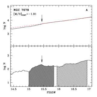
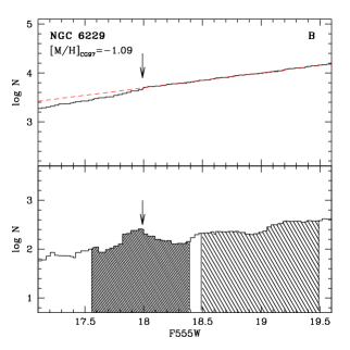
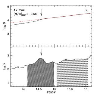
Figure 1: Example of the bump detection in three clusters. Panel A - The two panels show the cumulative (top) and differential (bottom) RGB LF for the metal poor cluster NGC 7078; Panel B - As in Panel A, but for the intermediate metallicity cluster NGC 6229; Panel C - As in Panel A, but for the metal rich cluster 47 Tuc. The global metallicity on the CG97 scale (see the text for details) is shown in each panel. The bump position (marked by the arrow) clearly shows up as a change in the slope of the cumulative LF, and it is confirmed by the differential LF.

2.1 Measurement of the $\Delta\mathrm{F555W}^{\mathrm{bump}}_{\mathrm{HB}}$ parameter

The parameter $\Delta\mathrm{F555W}^{\mathrm{bump}}_{\mathrm{HB}}$ used in this work is defined as the difference between the RGB bump and Zero Age HB (ZAHB) HST F555W magnitudes; it is therefore necessary to detect the bump along the cluster RGB and evaluate the ZAHB brightness at the level of the RR Lyrae instability strip, following Z99.

To measure the position of the RGB bump we used both the cumulative and differential LFs corrected using the completeness functions for the RGB sequences obtained from the artificial star experiments (Piotto et al. snapshot (2002)). For those clusters from which more populous samples of RGB stars were obtained (e.g. the 26 clusters marked with an asterisk in Tab. 1) the cumulative LF alone provides a solid determination of the bump level, which is always consistent with the existence of a statistically significant bump in the differential LF (see Fig. 1 for three examples). In case of the less populated clusters, both cumulative and differential LF have to be used simultaneously in order to estimate the bump level, as first discussed by Fusi Pecci et al. (1990). As discussed in sections 4.1 and 4.2, the bump detections in the more poorly sampled clusters are genuine, and in general, our detections for the whole sample are internally consistent.

We detected the RGB bump in 54 clusters, whereas for 20 other clusters this was not possible due either to poor RGB statistics, or to a large differential reddening, or to high field star contamination, especially for bulge clusters.

Fig. 1 shows some examples of the bump identification in the differential and in the cumulative LFs for three clusters in our database: a metal-poor cluster (NGC 7078, [M/H]${}_{\mathrm{CG97}}=-1.91$), an intermediate-metallicity (NGC 6229, [M/H]${}_{\mathrm{CG97}}=-1.09$), and a metal-rich one (47 Tuc, [M/H]${}_{\mathrm{CG97}}=-0.56$). In all panels, the position of the bump is marked by a vertical arrow.

The error bars on the bump position have been estimated by adding in quadrature the photometric error at the bump magnitude and the half width of the bin size used in the RGB LF.

Estimation of the ZAHB luminosity is a risky procedure due to the variety of HB morphologies and also to the fact that we cannot directly evaluate the mean magnitude of the RR Lyrae stars from our photometry. In fact, our photometric data cover only a very short time interval and this does not allow a suitable sampling of the pulsation cycle of the variables. Therefore, we followed the same procedure adopted by Z99. It can be briefly summarized as follows:

• clusters with $\mathrm{[Fe/H]}\leq-1$ (metal-intermediate and metal-poor): we divided the sample into metallicity groups (each group spans at most 0.2 dex in metallicity); to each metallicity group we associated a template cluster (with a metallicity within the group); the template clusters have accurate photometry and, most importantly, a sizable number of RR Lyrae, so that we could obtain an accurate estimate of the RR Lyrae magnitude level. Then we registered the HB of each cluster in the group to the HB of the reference cluster by artificially shifting the CMD of the template cluster in both color and magnitude in order to overlap both their RGBs and HBs. The mean magnitude of the RR Lyrae for each cluster was then obtained by shifting the RR Lyrae magnitude of the reference cluster by the magnitude difference adopted to overlap the two CMDs. Finally, we transformed the RR Lyrae mean magnitude into the ZAHB magnitude following Cassisi & Salaris (1997; see Z99 and Recio-Blanco et al. zahb (2003) for further details);

• clusters with $\mathrm{[Fe/H]}>-1$ (metal-rich) : we first estimated the photometric error ($\sigma_{\mathrm{F555W}}$) at the level of the HB using our set of artificial star experiments; then we determined the lower envelope of the HB stellar distribution. The ZAHB magnitude was eventually fixed at $3\sigma_{\mathrm{F555W}}$ magnitudes above the lower envelope.

The individual ZAHB luminosities as well as a more detailed description of the adopted procedure will be discussed in a companion paper (Recio-Blanco et al. 2003, in preparation).

The errors in $\Delta\mathrm{F555W}^{\mathrm{bump}}_{\mathrm{HB}}$  have been estimated by summing in quadrature the errors in the bump position $\mathrm{F555W}_{\mathrm{bump}}$ and in the ZAHB level $\mathrm{F555W}_{\mathrm{ZAHB}}$.

Because of the uncertainty that still affects the metallicity scale for GGCs (Rutledge, Hesser & Stetson rhs97 (1997); VandenBerg v00 (2000); Caputo & Cassisi cc02 (2002) and Kraft & Ivans ki03 (2003)), we have used both the Carretta & Gratton (cg97 (1997), hereinafter CG97) and the Zinn & West (zw84 (1984), hereinafter ZW84) metallicity scale. Moreover, we adopt, due to the lack of individual spectroscopic measurements for several GGCs in our sample, a mean $\alpha$-enhancement of 0.3 dex for metal-poor and metal-intermediate clusters $(\mathrm{[Fe/H]}<-1.0)$ and of 0.2 dex for metal-rich clusters $(\mathrm{[Fe/H]}>-1.0)$. The former value was suggested by Carney (carney (1996), C96), while the latter is a mean between the estimates collected by C96 and those collected by Salaris & Cassisi (sc96 (1996)). For each metallicity scale, the global cluster metallicity was estimated by using the relation provided by Salaris, Chieffi & Straniero (scs93 (1993)). We adopt a global metallicity error of $\pm$ 0.15 dex. This value can be considered as a safe lower limit to the uncertainties affecting both $\mathrm{[Fe/H]}$ and $[\alpha/\mathrm{Fe}]$ measurements (Rutledge et al. rhs97 (1997)).

Table 1 lists the relevant data for all clusters in our sample where the RGB bump has been detected. Column (1) gives the identification, columns (2) and (3) give the cluster global metallicity according to the metallicity scale provided by CG97, and by ZW84, respectively. Column (4) lists the F555W magnitude of the RGB LF bump, column (5) lists the $\Delta\mathrm{F555W}^{\mathrm{bump}}_{\mathrm{HB}}$ values with associated errors.

2.2 Measurement of the $R_{\mathrm{bump}}$ paramenter

We measured the $R_{\mathrm{bump}}$ parameter (using the same definition of B01 but the F555W magnitude) for all the 54 GGCs where we detected the bump. The star counts in the bump and in the normalization regions were corrected using the completeness functions given by the artificial star experiments.

The stellar counts in Bump and Normalization area are listed in columns (6) and (7) of Tab. 1, respectively. The values of the $R_{\mathrm{bump}}$ parameter with the corresponding errors are listed in column (8). The 1$\sigma$ error on the observed $R_{\mathrm{bump}}$ values is determined according to $\sigma$($R_{\mathrm{bump}}$)=$R_{\mathrm{bump}}$ $\sqrt{(1/N_{b})+(1/N_{n})}$ where $N_{b}$ and $N_{n}$ are the star counts in the bump and in the normalization region, respectively.

3 The theoretical framework

The theoretical framework we adopt in this investigation is based on an updated and larger set of stellar models (Pietrinferni, Cassisi, Salaris & Castelli 2003). The new models have been computed by using a recent version of the FRANEC evolutionary code. The input physics has been updated with respect to the models used in Z99 (Cassisi & Salaris 1997), and the changes are summarized in the following:

• the radiative opacity is obtained from the OPAL tables (Iglesias & Rogers iglesias (1996)) for temperatures larger than $10^{4}$ K, and from Alexander & Ferguson (alexander (1994)) for lower temperatures. Opacity for electron degenerate matter is computed following Potekhin (pot (1999)).

• We updated the energy loss rates for plasma-neutrino processes by using the most recent and accurate results provided by Haft, Raffelt & Weiss (haft (1994)). For all other processes we still rely on the same prescriptions adopted by Cassisi & Salaris (1997).

• The nuclear reaction rates have been updated by using the NACRE database (Angulo et al. 1999), with the exception of the ¹²C$(\alpha,\gamma)^{16}$O reaction. For this reaction we employ the more accurate recent determination by Kunz et al. (kunz (2002)).

• The detailed Equation of State (EOS) by A. Irwin has been used. A full description of this EOS is still in preparation (Irwin et al. 2003) but a brief discussion of its main characteristics can be found in Cassisi, Salaris & Irwin (csi03 (2003)). It is enough to mention here that this EOS, whose accuracy and reliability is similar to the OPAL EOS developed at the Livermore Laboratories (Rogers, Swenson & Iglesias rsi96 (1996)) and recently updated in the treatment of some physical inputs (Rogers & Nayfonov rn02 (2002)), allows us to compute self-consistent stellar models in all evolutionary phases relevant to this investigation.

• The extension of the convective zones is fixed by means of the classical Schwarzschild criterion. Induced overshooting and semiconvection during the He-central burning phase are accounted for following Castellani et al. (cast85 (1985)). The thermal gradient in the superadiabatic regions is determined according to the mixing length theory, whose free parameter has been calibrated by computing a solar standard model.

• Our evolutionary code includes the process of atomic diffusion of both Helium and heavy elements; the models used in this work, however, have been computed with the atomic diffusion switched off, taking into account that Cassisi et al. (cds97 (1997)) have clearly shown how the effect of this physical process on $\Delta{V}^{\mathrm{bump}}_{\mathrm{HB}}$is negligible.

• We adopt a scaled-solar heavy element mixture (Grevesse & Noels gn93 (1993)); the enhancement of $\alpha$-elements observed in GGCs is accounted for following the prescriptions by Salaris et al. (scs93 (1993)).

• As far as the initial He-abundance is concerned, we adopt the estimate recently provided by Cassisi et al. csi03 (2003) on the basis of new measurements of the $R$ parameter in a large sample of GGCs. They found an initial He-abundance for GGC stars of the order of $Y=0.245$, which is in fair agreement with recent empirical measurements of the cosmological baryon density provided by W-MAP (Spergel et al. 2003). To reproduce the calibrated initial solar He-abundance we used $dY/dZ\approx 1.4$ (Pietrinferni et al. 2003).

• Bolometric magnitudes have been transformed into HST F555W magnitudes according to the transformations provided by Origlia & Leitherer (origlia (2000)), based on the atmosphere models computed by Bessell, Castelli & Plez (bcp98 (1998)).

A more detailed discussion about the model input physics and the evolutionary code is presented in Pietrinferni et al. (2003).

Finally, we discuss in more detail the metal distribution used to compute the evolutionary models. In our analysis we will compare the models computed with a scaled-solar metal abundance to GGCs data for which the metal abundance is $\alpha$-enhanced. According to Salaris et al. (1993), as long as the $\alpha$-elements have approximately the same enhancement, scaled-solar models mimic $\alpha$-enhanced models computed with the same global metallicity [M/H]. This is, however, strictly true only for [M/H] values up to $\sim-$1.0, as shown by Salaris & Weiss (1998) and Vandenberg et al. (2000). For higher global metallicities this equivalence is not well satisfied anymore. Therefore we investigated how different would be the $\Delta\mathrm{F555W}^{\mathrm{bump}}_{\mathrm{HB}}$ parameter at a given [M/H] larger than $-$1, for a scaled-solar and an $\alpha$-enhanced metal mixture. We used isochrones by Salaris & Weiss (1998) with [M/H]=$-$0.3 (approximately the upper end of the metallicity range spanned by our GGC sample), both scaled-solar and with [$\alpha$/Fe]=0.4; we found that the $\Delta\mathrm{F555W}^{\mathrm{bump}}_{\mathrm{HB}}$ values are changed by only 0.05 mag for typical GGC ages, the $\alpha$-enhanced ones being larger. This is however just an upper limit to the real difference, since these metal rich clusters seem to show an $\alpha$-enhancement lower than [$\alpha$/Fe]=0.4. We conclude that, as far as the $\Delta\mathrm{F555W}^{\mathrm{bump}}_{\mathrm{HB}}$ parameter is concerned, we can safely use scaled-solar models with the cluster global [M/H] even in the high metallicity regime. We also verified that the $R_{\mathrm{bump}}$ values are unaffected by the $\alpha$-enhanced metal distribution.

Table 2: Theoretical $\Delta\mathrm{F555W}^{\mathrm{bump}}_{\mathrm{HB}}$ values as a function of $[M/H]$ and age.

$[M/H]$	$\Delta\mathrm{F555W}^{\mathrm{bump}}_{\mathrm{HB}}$
	$10$ Gyr	$12$ Gyr	$14$ Gyr	$16$ Gyr.
-2.267	-0.907	-0.846	-0.770	-0.699
-1.790	-0.690	-0.621	-0.555	-0.494
-1.266	-0.297	-0.221	-0.159	-0.116
-0.963	-0.056	0.004	0.056	0.108
-0.659	0.192	0.271	0.347	0.418
-0.253	0.469	0.566	0.649	0.694
0.000	0.639	0.741	0.791	0.843

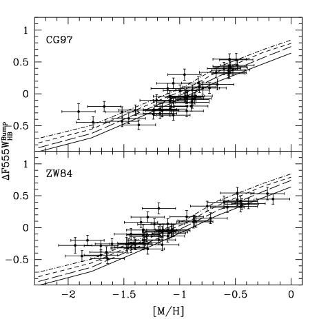
Figure 2: Comparison between the theoretical and empirical values of $\Delta\mathrm{F555W}^{\mathrm{bump}}_{\mathrm{HB}}$ as a function of the global metallicity for all the 54 GGCs in our sample (left panel) and for the 26 GGCs with more than 85 stars in the bump region (right panel). The empirical $\Delta\mathrm{F555W}^{\mathrm{bump}}_{\mathrm{HB}}$ data are plotted as a function of both the Zinn & West (zw84 (1984) – ZW84) and Carretta & Gratton (cg97 (1997) – CG97) metallicity scales (see text for more details). The theoretical predictions are plotted for four different cluster ages, namely 10 Gyr (solid line), 12 Gyr (long dash), 14 Gyr (short dash), and 16 Gyr (dot - short dash).

4 Comparison between theory and observations

4.1 The $\Delta\mathrm{F555W}^{\mathrm{bump}}_{\mathrm{HB}}$ parameter

Figure 2 shows the comparison between theoretical predictions (given in Tab. 2) and measured values of $\Delta\mathrm{F555W}^{\mathrm{bump}}_{\mathrm{HB}}$  as a function of the global metallicity [M/H], for a selected age range. The behaviour of the theoretical $\Delta\mathrm{F555W}^{\mathrm{bump}}_{\mathrm{HB}}$ stems from the strong dependence of the depth of the convective envelope on both metallicity and mass. The higher the cluster age, the smaller the evolving mass along the RGB, with an ensuing deeper extension of the convective envelope, and a fainter bump brightness, whereas the HB level is largely unaffected. On the other hand, at a fixed age, the larger the metallicity, the deeper the extension of the convective envelope which causes a fainter bump; the HB is also fainter for increasing metallicity, but the effect on the bump level is larger, thus causing an increase of $\Delta\mathrm{F555W}^{\mathrm{bump}}_{\mathrm{HB}}$.

The left panel of Fig. 2 shows the data for the entire sample of GCs, whereas in the right panel we plot only the clusters with more than 85 stars in the bump region (hereafter we will refer to this sample of clusters as the best cluster sample). A glance at this figure reveals that the distribution of the observational data for the entire sample closely resembles the distribution for the best cluster sample which, incidentally, spans the entire metallicity range covered by the full sample. This evidence supports the significance of the bump detections for the whole 54 clusters listed in Tab. 1. Further confirmation comes from the fact that, as we will see in the following, the comparison with theory provides exactly the same results when considering either the full sample or the best cluster sample. We anticipate that the analysis of the $R_{\mathrm{bump}}$ parameter, presented in the next subsection, will provide additional evidence for the significance of the bump detection in all the clusters displayed in Table 1.

Figure 2 shows also a qualitative agreement between observations and theory. In particular, both theoretical lines and observations lie in the same region of the $\Delta\mathrm{F555W}^{\mathrm{bump}}_{\mathrm{HB}}$[M/H] plane, and the observed trend with metallicity is well reproduced by theory (with the possible exception of the three most metal poor clusters).

We have also performed a more quantitative comparison, though it must be noted that it is made difficult (and uncertain) by the strong dependence of $\Delta\mathrm{F555W}^{\mathrm{bump}}_{\mathrm{HB}}$ on the cluster age and metal content. Indeed, $\Delta\mathrm{F555W}^{\mathrm{bump}}_{\mathrm{HB}}$ varies by 0.03 magnitudes for a 1 Gyr variation in age, and by the same amount for a variation of only 0.04 dex in [M/H]. To assess the internal accuracy of theoretical models we compared the cluster age required to fit the observed $\Delta\mathrm{F555W}^{\mathrm{bump}}_{\mathrm{HB}}$ values with the age determinations obtained from the main sequence (MS) turn off (TO) position. It must be explicitly noted that we do not propose to use the $\Delta\mathrm{F555W}^{\mathrm{bump}}_{\mathrm{HB}}$ parameter as an age indicator; however, we should expect that, for any given metallicity scale, the age scale inferred from the $\Delta\mathrm{F555W}^{\mathrm{bump}}_{\mathrm{HB}}$ agrees with the ages from the TO. Systematic or random age offsets imply (systematic or random) effects not properly accounted for by the models.

We started with the CG97 metallicity scale. The theoretical line which best fits the observed distribution of $\Delta\mathrm{F555W}^{\mathrm{bump}}_{\mathrm{HB}}$ with the metallicity has an age of $11.8$ Gyr, with a 1$\sigma$ dispersion of 4.0 Gyr. Figure 3 (upper panel) displays the comparison between the observed $\Delta\mathrm{F555W}^{\mathrm{bump}}_{\mathrm{HB}}$ and the models for the labeled age. The use of only the best cluster sample (26 objects) sample does not affect the age, though the spread is slightly reduced. A close inspection of Fig. 3 shows that clusters with [M/H]$<-$1.6 are systematically discrepant, even those with the best populated bump. This fact may point out to some serious inaccuracy of the stellar models for this metallicity range, though we cannot exclude that the discrepancy may be ascribed to a different ‘true’ global metallicity for these clusters (e.g., the $\alpha$-enhancement is higher than assumed). Moreover, the discrepant clusters in this metallicity range are only a few, namely M 15, M 68, and M 53. A larger sample of metal-poor clusters with a well-populated RGB is required before a definitive conclusion on this possible discrepancy can be reached.

If we restrict our analysis to the clusters with [M/H]$>-$1.6, the best fitting model corresponds to an age of $\approx 11$ Gyr, which does not change when we consider only objects belonging to the best cluster sample. The dispersion of the data points around this best fitting model does, however, decreases from 3.4 to 2.6 Gyr when using the best sample. Most interestingly, we also found that the age scatter around the best fitting model does not correlate significantly with [M/H].

A different result is obtained using the ZW84 metallicity scale. In this case, the age of the best fitting model is $\approx 15$ Gyr (Fig. 3), but now the residuals show a correlation with [M/H]. In order to obtain a better match with the theoretical $\Delta\mathrm{F555W}^{\mathrm{bump}}_{\mathrm{HB}}$  a younger age for more metal-rich clusters must be used. More specifically, we find an overall statistically significant age-[M/H] relationship, with a slope $(-5.7\pm 1.1)\rm Gyr\leavevmode\nobreak\ dex^{-1}$. If we neglect the three most metal-poor clusters mentioned above (they have [M/H]$<-$1.8 in the ZW84 scale), we obtain a slope $(-4.8\pm 1.1)\rm Gyr\leavevmode\nobreak\ dex^{-1}$, which does not change for the best cluster sample (with [M/H]$>-$1.8). In this case, the best fitting model correspond has an age of $\approx 14$ Gyr.

In summary, when using the CG97 scale the cluster average age is of 11-12 Gyr, in agreement with the TO ages obtained by Salaris & Weiss (2002), who determine the GGC distances from their theoretical models. Using the same metallicity scale, and measuring distances with the classical MS fitting technique, Carretta et al. (2000) find a similar age (though their best age estimate is roughly 13 Gyr, when they consider also other independent distance scales) . A second result of the comparison shown in Fig. 3 is that, when using the CG97 metallicity scale, we do not find any statistically significant age-metallicity trend from the $\Delta\mathrm{F555W}^{\mathrm{bump}}_{\mathrm{HB}}$ parameter, whereas Rosenberg et al. (alfred (1999)), VandenBerg (2000), Salaris & Weiss (2002), find in general that the more metal rich clusters are younger, and Gratton et al. (g03 (2003)) find that the metal-rich cluster 47 Tuc is about 2.6 Gyr younger than more metal-poor clusters like NGC 6752.

Salaris & Weiss (2002) obtain, on average, ages higher by about 1 Gyr when moving from the CG97 to the ZW84 metallicity scale, but still lower than the age derived from the $\Delta\mathrm{F555W}^{\mathrm{bump}}_{\mathrm{HB}}$. VandenBerg (2000) determines ages of about 14 Gyr for the oldest metal-poor GGCs using his own HB models and the ZW84 scale, and ages decreasing on average when moving to the higher metallicity regime. These results confirms the earlier work by Rosenberg et al. (alfred (1999)), who find that the most metal rich clusters are 15-20% younger than the most metal poor ones. In conclusion, the age-metallicity relationship we found from $\Delta\mathrm{F555W}^{\mathrm{bump}}_{\mathrm{HB}}$ when adopting the ZW84 metallicity scale, is in qualitative agreement with the results we obtain from the TO ages, but the slope is larger. Also the average age implied by the $\Delta\mathrm{F555W}^{\mathrm{bump}}_{\mathrm{HB}}$ parameter seems larger than the most recent determinations.

Unfortunately, this analysis provides somewhat not definitive results about the accuracy of the theoretical $\Delta\mathrm{F555W}^{\mathrm{bump}}_{\mathrm{HB}}$ values. This is due mainly to the current uncertainties in the cluster metallicities and, to a minor extent, to uncertainties in the GGC ages (which depend themselves on the metallicity errors). In fact, typical differences among the TO absolute GGC ages mentioned before are of the order of 1-2 Gyr; these differences affect $\Delta\mathrm{F555W}^{\mathrm{bump}}_{\mathrm{HB}}$ (at a given [M/H]) at the level of 0.03-0.06 mag, whereas typical differences of 0.2 dex between the CG97 and ZW84 [M/H] scale modify $\Delta\mathrm{F555W}^{\mathrm{bump}}_{\mathrm{HB}}$ (at a fixed age) by $\sim$0.2 mag.

Figure 3: Comparison between observed and predicted $\Delta\mathrm{F555W}^{\mathrm{bump}}_{\mathrm{HB}}$ values for the labeled average ages determined in case of, respectively, the CG97 (upper panel) and ZW84 (lower panel) [M/H] scale. Filled circles denote the 26 GGCs with more than 85 stars in the bump region, whereas open circles represent the remaining clusters in our sample.

Figure 4: Comparison between the theoretical and empirical values of $R_{\mathrm{bump}}$ as a function of the global metallicity for all the GGCs in our sample; symbols are as in Fig. 3. The bottom and upper panels refer, respectively, to the ZW84 and CG97 [M/H] scale. The solid lines show the theoretical values for 10 (upper line) and 16 Gyr.

4.2 The $R_{\mathrm{bump}}$ parameter

The comparison between theoretical predictions and empirical measurements of the $R_{\mathrm{bump}}$ parameter is shown in Fig. 4, for the same two metallicity scales discussed before. It is important to remark that, as in case of $\Delta\mathrm{F555W}^{\mathrm{bump}}_{\mathrm{HB}}$  the $R_{\mathrm{bump}}$ distribution for the clusters with the most populated bump region does not show any evident systematic offset when compared to the full sample. Due to the fact that one expects a weak dependence of $R_{\mathrm{bump}}$ on both [M/H] and age, it is meaningful to compare the mean measured $R_{\mathrm{bump}}$ values for the best cluster sample and the full sample. The mean value of $R_{\mathrm{bump}}$ for the latter is 0.498$\pm$0.092 (1$\sigma$ dispersion); in case of selecting only the 26 objects belonging to the best cluster sample (which corresponds to clusters with $\sigma$($R_{\mathrm{bump}}$)/$R_{\mathrm{bump}}$below 13%) we obtain 0.497$\pm$0.064, practically identical to the value for the whole sample, but with a smaller dispersion because of smaller individual error bars (due to Poisson fluctuations in the values of $N_{b}$ and $N_{n}$). This is another clear evidence for the significance of our bump detections. In fact, in case of spurious detections in the less populated clusters, caused by random fluctuations in the number of RGB stars, we would expect to obtain an average $R_{\mathrm{bump}}$ value equal to $\sim$0.37 (corresponding to models where the H-abundance jump is absent) with a given dispersion around this value due to Poisson noise; however, when we consider only the less populated clusters with $\sigma$($R_{\mathrm{bump}}$)/$R_{\mathrm{bump}}$ larger than 13%, we obtain a distribution of points with a mean value of 0.498 equal to the best cluster sample, and not centred around 0.37.

To test the consistency of the observed $R_{\mathrm{bump}}$ with theory, we adopted the following approach: for a given metallicity scale we computed, on a cluster by cluster basis, the corresponding theoretical $R_{\mathrm{bump}}$ values, using the ages obtained from $\Delta\mathrm{F555W}^{\mathrm{bump}}_{\mathrm{HB}}$. The precise age value is however not crucial, due to the very low sensitivity of the $R_{\mathrm{bump}}$ parameter to age (see the discussion in B01 and data plotted in Fig. 4). Also the dependence on [M/H] is very weak, as noticed before.

These 54 theoretical values have been compared with the empirical data and the difference between theory and observations has been analyzed (see Fig. 5). We found an average difference (theory-observations) $\Delta$($R_{\mathrm{bump}}$)=$-0.002\pm$0.093 (1$\sigma$) for the whole GGC sample when using the CG97 metallicity scale, with no evident correlation of the residuals with [M/H]. We also tested, making use of Monte Carlo simulations, if the dispersion around the mean can be explained by the Poisson errors on the empirical determination of $R_{\mathrm{bump}}$. More in detail, for each cluster we randomly generated 10000 values of $\Delta$($R_{\mathrm{bump}}$), centred around $-$0.002 and with a Gaussian 1$\sigma$ dispersion equal to the observational error on $R_{\mathrm{bump}}$. We then joined together the synthetic $\Delta$($R_{\mathrm{bump}}$) values for each individual cluster, and determined the 1$\sigma$ dispersion of the resulting distribution, which compares well with the observed value of 0.093. We also considered, as a further test, the subsample of 26 clusters with the best populated RGB up to the bump region. The $R_{\mathrm{bump}}$ residuals show again a negligible difference from zero, the average value being $-0.002\pm$0.065, and once again we found that the dispersion around this value can be explained as observational errors on the $R_{\mathrm{bump}}$ parameter. Note the much smaller value of the dispersion when only the best $R_{\mathrm{bump}}$ determinations are accounted for. We obtain the same result if M 15 and M 53 – the two most metal poor clusters – are neglected (see Fig. 5).

Figure 5: Difference between the theoretical $R_{\mathrm{bump}}$ values computed for the individual cluster ages determined from $\Delta\mathrm{F555W}^{\mathrm{bump}}_{\mathrm{HB}}$  and the observational counterpart, in case of the CG97 (upper panel) and ZW84 (lower panel) [M/H] scale. The horizontal dashed line corresponds to a zero difference and it is not a fit to the data.

When using the ZW84 scale, and the age distribution obtained from $\Delta\mathrm{F555W}^{\mathrm{bump}}_{\mathrm{HB}}$, the average value of the difference between theoretical and observed $R_{\mathrm{bump}}$ is slightly higher, namely $-0.028\pm$0.093, the residuals showing no trend with [M/H]. The average value is $-0.022\pm$0.064 if we consider the best cluster sample.

4.3 The effect of chemical self pollution

To explain the observed CNO abundance anomalies and the extended blue HB tail in some GGCs, D’Antona et al. (2002) suggested the existence of an He-enriched stellar component within the clusters, due to chemical pollution by the ejecta of massive asymptotic giant branch stars. We tested whether this He-enhancement might affect predicted $\Delta\mathrm{F555W}^{\mathrm{bump}}_{\mathrm{HB}}$ and $R_{\mathrm{bump}}$ values when compared to the case of a constant He-abundance. Following D’Antona et al. (2002) results, we have produced a synthetic CMD for an hypothetical 12 Gyr old GGC with [M/H]=$-$1.3. We considered that 64% of the coeval stellar population is composed of stars with the standard He-abundance adopted in our models, whereas 36% of the population is made of stars with Y randomly distributed between the standard value and an abundance 0.06 higher. We found that the location of the bump in the LF of this He-enhanced population does not show any significant difference with respect to the standard case. The HB level at the RR Lyrae instability strip – as shown by D’Antona et al. (2002) – is determined by the ’He-normal’ population, and therefore, the $\Delta\mathrm{F555W}^{\mathrm{bump}}_{\mathrm{HB}}$ value for a cluster with He-enhanced stars is expected to be very close to the case of a standard He-normal population. It is also important to notice that, if the He-enhanced stars have all the same abundance 0.06 higher than the bulk of the cluster population, the cluster LF would show a second bump, about 0.13 mag brighter than the main one.

As far as the $R_{\mathrm{bump}}$ parameter is concerned, we found only a a marginal difference. In conclusion, the occurrence of chemical pollution due to the same GGC stars does not affect the $\Delta\mathrm{F555W}^{\mathrm{bump}}_{\mathrm{HB}}$ and the $R_{\mathrm{bump}}$ values predicted by canonical stellar models.

5 Summary and final remarks

In this investigation we adopted a database of HST photometric data for a large sample of GGCs, and we have been able to measure the RGB bump location in a sample of 54 clusters. For the same cluster sample we have also determined the star counts in the bump region following B01. This represents, so far, the largest database of empirical estimates for both the RGB bump brightness and star counts in this evolutionary phase.

The observed magnitude difference between the bump and the HB, i.e. $\Delta\mathrm{F555W}^{\mathrm{bump}}_{\mathrm{HB}}$  and the star counts in the bump region, i.e. the $R_{\mathrm{bump}}$ parameter, have been compared with theoretical predictions by using a new set of stellar evolution models. To account for the current uncertainty in the GGC metallicity scale, we have adopted both the CG97 [Fe/H] scale and the ZW84 one. We also employed reasonable assumptions for the $\alpha$-element enhancement in GGCs stars, based on the presently available estimates.

Owing to the sensitivity of the $\Delta\mathrm{F555W}^{\mathrm{bump}}_{\mathrm{HB}}$ parameter on cluster age, the ages required to fit the observed $\Delta\mathrm{F555W}^{\mathrm{bump}}_{\mathrm{HB}}$ values should agree with recent independent estimates based on the luminosity of the TO, for the theoretical models being consistent with observations. Our results can be summarized as follows:

• The mean age needed to obtain agreement between observed and predicted $\Delta\mathrm{F555W}^{\mathrm{bump}}_{\mathrm{HB}}$  values is $\sim 12$ Gyrs (with a $1\sigma$ dispersion of 4.0 Gyrs) when the CG97 [Fe/H] scale is used. This value is slightly smaller than recent independent estimates obtained by using the same metallicity scale. It is also worth mentioning that a significant discrepancy exists for the most metal-poor clusters ([M/H]$\leq-1.6$) in our sample. Current data do not allow us to conclusively assess whether this represents a real problem for the theoretical models, or the discrepancy is due is an observational bias due to the limited sample of stars located along the RGB. At variance with results from studies of TO ages, the $\Delta\mathrm{F555W}^{\mathrm{bump}}_{\mathrm{HB}}$ of metal rich clusters like 47 Tuc is reproduced by models with the same average age as more metal poor ones.

• The mean cluster age is $\sim 15$ Gyr when the ZW84 [Fe/H] scale is used and, in addition, we find a statistically significant correlation between the residuals around this age and the cluster [M/H]. This mean age of 15 Gyr appears larger than similar mean GGC ages available in the literature. The slope of the age-metallicity relationship, though in qualitative agreement with current estimates (e.g., Rosenberg et al. alfred (1999) and Gratton et al. 2003), is also too steep.

On the basis of these results we can draw the following conclusion: even though a qualitative agreement between theory and observations of $\Delta\mathrm{F555W}^{\mathrm{bump}}_{\mathrm{HB}}$ does exist, a more definitive assessment of the confidence level is hampered by the not negligible uncertainties still affecting both the cluster [Fe/H] and [$\alpha$/Fe] estimates. More robust conclusions require more accurate spectroscopic measurements of these quantities.

As far as the $R_{\mathrm{bump}}$ parameter is concerned, our analysis suggests that there is a good agreement between theory and observations, regardless of the adopted metallicity scale. This result is also due to the weak dependence of this parameter on the cluster metallicity (and age), which minimizes the effects related to the uncertainties on the [M/H] scale.

Finally, we found that the effect on both $\Delta\mathrm{F555W}^{\mathrm{bump}}_{\mathrm{HB}}$ and $R_{\mathrm{bump}}$ of a possible He-rich component – as recently suggested by D’Antona et al. (2002) – in the cluster stellar population is negligible.

- (1) Alexander, D. R., & Ferguson, J. W. 1994, ApJ, 437, 879
- (2) Alves, D. R., & Sarajedini, A. 1999, ApJ, 511, 225
- (3) Angulo, C., et al. (NACRE Collaboration), 1999, Nuclear Physics A, 656, 3
- (4) Bergbusch, P. A., & Vandenberg, D. A. 2001, ApJ, 556, 322
- (5) Bessel, M. S., Castelli, F., & Plez, B. 1998, A&A, 333, 231
- (6) Bono, G., Cassisi, S., Zoccali, M., & Piotto, G. 2001, ApJ, 546, L109 (B01)
- (7) Caputo, F., & Cassisi, S. 2002, MNRAS, 333, 825
- (8) Carney, B. W. 1996, PASP, 108, 900 (C96)
- (9) Carretta, E., & Gratton, R. G. 1997, A&AS, 121, 95 (CG97)
- (10) Carretta, E., Gratton, R. G., Clementini, G., Fusi Pecci, F. 2000, ApJ, 533, 215
- (11) Cassisi, S., Degl’Innocenti, S., & Salaris, M. 1997, MNRAS, 290, 515
- (12) Cassisi, S., & Salaris, M. 1997, MNRAS, 285, 593
- (13) Cassisi, S., Salaris, M., & Bono, G. 2002, ApJ, 565, 1231
- (14) Cassisi, S., Salaris, M., & Irwin, A. W. 2003, ApJ, 588, 852
- (15) Castellani, V., Chieffi, A., Tornambe, A., & Pulone, L. 1985, ApJ, 296, 204
- (16) Castellani, V. 1999, in ”Globular clusters”, Proceedings of the X Canary Islands Winter School of Astrophysics, C. Martinez Roger, I. Perez Fournón & F. Sánchez eds., p. 109
- (17) D’Antona, F., Caloi, V., Montalban, J., Ventura, P., & Gratton, R.G. 2002, A&A, 395, 69
- (18) Dolphin, A. E. 2000, PASP, 112, 1397
- (19) Ferraro, F. R., Messineo, M., Fusi Pecci, F., de Palo, M. A., Straniero, O., Chieffi, A., & Limongi, M. 1999, AJ, 118, 1738
- (20) Fulton, L. K., Carney, B. W., Olzewski, E. W., Zinn, R., Demarque, P., Janes, K. A., Da Costa, G. S., & Seitzer, P. 1995, AJ, 110, 652
- (21) Fusi Pecci, F., Ferraro, F. R., Crocker, D. A., Rood, R. T., & Buonanno, R. 1990, A&A, 238, 95
- (22) Gratton, R. et al. 2003, A&A, in press (astro-ph/0307016)
- (23) Grevesse, N., & Noels, A., 1993, in: Prantzos, N., Vangioni-Flam, E., Casse, M. (eds.) , Origin and Evolution of the Elements, (Cambridge University Press), 15
- (24) Haft, M., Raffelt, G., & Weiss, A. 1994, ApJ, 425, 222
- (25) King, C. R., Da Costa, G. S., & Demarque, P. 1985, ApJ, 299, 674
- (26) Kraft, R. P. & Ivans, I. I. 2003, PASP, 115, 143
- (27) Kunz, R., Fey, M., Jaeger, M., Mayer, A., Hammer, J. W., Staudt, G., Harissopulos, S., & Paradellis, T. 2002, ApJ, 567, 643
- (28) Iben, I., Jr. 1968, ApJ, 154, 581
- (29) Iglesias, C. A., & Rogers, F. J. 1996, ApJ, 464, 943
- (30) Irwin, A. W. et al. 2003, in preparation
- (31) Origlia, L. & Leitherer, C. 2000, AJ, 119, 2018
- (32) Pietrinferni, A., Cassisi, S., Salaris, M. & Castelli, F. 2003, in preparation
- (33) Piotto, G., King, I. R., Djorgovski, S. G., Sosin, C., Zoccali, M., Saviane, I., De Angeli, F., Riello, M., Recio-Blanco, A., Rich, R. M., Meylan, G., & Renzini, A. 2002, A&A, 391, 945
- (34) Potekhin, A.Y. 1999, A&A, 351, 787
- (35) Recio Blanco, A., et al. 2003 in preparation
- (36) Renzini, A., & Fusi Pecci, F. 1988, ARA&A, 26, 199
- (37) Rogers, F. J., Swenson, F. J., & Iglesias, C. A. 1996, ApJ, 456, 902
- (38) Rogers, F. J., & Nayfonov, A. 2002, ApJ, 576, 1064
- (39) Rosenberg, A., Saviane, I., Piotto, G., & Aparicio, A. 1999, AJ, 118, 2306
- (40) Rutledge, G. A., Hesser, J. E., & Stetson, P. B. 1997, PASP, 109, 907
- (41) Salaris, M., Chieffi, A., & Straniero, O. 1993, ApJ, 414, 580
- (42) Salaris, M., & Cassisi, S. 1996, A&A, 305, 858
- (43) Salaris, M., & Weiss, A. 1998, A&A, 335, 943
- (44) Salaris, M., Cassisi, S., & Weiss, A. 2002, PASP, 114, 375
- (45) Salaris, M., & Weiss, A. 2002, A&A, 388, 492
- (46) Spergel, D.N. et al. 2003, ApJ, in press
- (47) Thomas, H. C. 1967, Ph.D. thesis, L. M. Univ., Münich
- (48) VandenBerg, D. A. 2000, ApJS, 129, 315
- (49) VandenBerg., D.A., Swenson, F.J., Rogers, F.J., Iglesias, C.A., & Alexander, D.R. 2000, ApJ, 532, 430
- (50) Zinn, R., & West, M. J. 1984, ApJS, 55, 45 (ZW84)
- (51) Zoccali, M., Cassisi, S., Piotto, G., Bono, G., & Salaris, M. 1999, ApJ, 518, L49 (Z99)