Prospects for Spectroscopic Reflected-light Planet Searches

Abstract

High-resolution spectroscopic searches for the starlight reflected from close-in extra-solar giant planets have the capability of determining the optical albedo spectra and scattering properties of these objects. When combined with radial velocity measurements they also yield the true mass of the planet. To date, only two such planets have been targeted for reflected-light signals, yielding upper limits on the planets’ optical albedos. Here we examine the prospects for future searches of this kind. We present Monte Carlo estimates of prior probability distributions for the orbital velocity amplitudes and planet/star flux ratios of 6 bright stars known to harbour giant planets in orbits with periods of less than 5 days. Using these estimates, we assess the viability of these targets for future reflected-light searches using 4m and 8m-class telescopes.

Key Words: Planets: extra-solar - Planets: atmosphere - Planets: reflected-light

1 Introduction

Spectral models of close-orbiting giant exoplanets [Seager & Sasselov1998, Marley, Gelino & Stephens1999, Goukenleuque, Bezard & Lellouch1999, Sudarsky, Burrows & Pinto2000, Barman, Hauschildt & Allard2001, Sudarsky, Burrows & Hubeny2003, Baraffe et al.2003] show that scattered starlight dominates over thermal emission at optical wavelengths, but the albedo is very sensitive to the depth of cloud formation. sudarsky2000 find that the relatively low surface gravities of planets such as $\upsilon$ Andromeda b, HD 75289 b and HD 209458 b may favour the formation of relatively bright, high-altitude silicate cloud decks. On higher-gravity objects such as $\tau$ Bootis b, however, the same models predict a much deeper cloud deck. In this case, much of the optical spectrum is absorbed by the resonance lines of the alkali metals. The Na I D lines in particular are strongly broadened by collisions with $H_{2}$ molecules.

In reality, however, the atmospheric structure of close-orbiting giant planets (hereafter “Pegasi Planets”) is expected to be more complex, with strong winds and horizontal temperature variations [Showman & Guillot2002], and possible temporal variations [Cho et al.2003]. The combined atmospheric circulation and temperature variations are likely to yield a disequilibrium chemical composition. Furthermore, the location and characteristics of any cloud decks cannot be predicted to any great precision with present theoretical knowledge. The next logical step towards understanding the properties and evolution of these objects will be to test these emerging models by measuring the albedos of these Pegasi planets directly.

A planet of radius $R_{p}$ orbiting a distance $a$ from a star intercepts a fraction $\left(R_{p}/2a\right)^{2}$ of the stellar luminosity. The proximity of Pegasi planets to their parent stars make them excellent prospects for reflected-light searches. At optical wavelengths, starlight scattered off the planet’s atmosphere is expected to dominate over thermal emission. charb99,cameron99 showed that the planet/star flux ratio

$$\varepsilon(\alpha,\lambda)\equiv\frac{f_{p}(\alpha,\lambda)}{f_{\star}(\lambda)}=p(\lambda)\left(\frac{R_{p}}{a}\right)^{2}g\left(\alpha,\lambda\right)$$ (1)

is expected to vary with the star-planet-observer illumination angle $\alpha$, giving a small periodic modulation to the system brightness in the form of the phase function $g(\alpha,\lambda)$. Here $p(\lambda)$ represents the geometric albedo of the planet’s atmosphere that, like the phase function, is wavelength ($\lambda$) dependent. Assuming a grey albedo model, i.e. no wavelength dependence, the amplitude of optical flux variability for a typical Pegasi planet system is expected to be

$$\frac{\Delta f}{f}\leq 8.3\times 10^{-5}\left(\frac{p}{0.4}\right)\left(\frac{R_{p}/1.4R_{Jup}}{a/0.045AU}\right)^{2}$$ (2)

Future space-based photometry missions are expected to be able to detect and measure this modulation with ease. However, the orbital inclination (and hence planet’s mass) cannot be determined directly form the light-curve, since the form of the phase function $g(\alpha,\lambda)$ is unknown.

2 Spectroscopic reflected-light searches

Star	Spectral	$m_{V}$	$T_{eff}$	$P_{rot}$	$v\sin{i}$	[Fe/H]	Age	$M_{*}/M_{\odot}$	$R_{*}/R_{\odot}$
	Type	(Mags)	(K)	(Days)	$(km.s^{-1})$		(Gyrs)
$\upsilon$ And	F8V 1	4.09	6107$\pm$80 4	12.2$\pm$2 6	9.3$\pm$0.4 4	0.09$\pm$0.06 4	3.8$\pm$1.0 4	1.27$\pm$0.06 14	1.67$\pm$0.06 14
$\tau$ Boo	F7V 1	4.50	6360$\pm$80 4	3.3$\pm$0.1 7	14.8$\pm$0.3 4	0.27$\pm$0.08 4	1.0$\pm$0.6 4	1.37$\pm$0.05 14	1.46$\pm$0.06 14
51 Peg	G2V 1	5.46	5793$\pm$70 4	29$\pm$7 6	2.1$\pm$0.7 4	0.20$\pm$0.07 4	4.0$\pm$2.5 4	1.10$\pm$0.06 14	1.20$\pm$0.07 14
HD 179949	F8V 2	6.25	6115$\pm$50 5	9$\pm$2 8	6.3$\pm$0.9 9	0.22$\pm$0.07 11	3.5$\pm$2.5 13	1.24$\pm$0.10 14	1.24$\pm$0.10 14
HD 75289	G0V 3	6.35	6000$\pm$50 3	16$\pm$3 8	4.4$\pm$1.0 10	0.29$\pm$0.08 12	5.6$\pm$1.0 12	1.22$\pm$0.05 14	1.25$\pm$0.05 14
HD 209458	F9V 1	7.65	6000$\pm$50 8	16.5$\pm$3 18	3.7$\pm$1.3 17	0.00$\pm$0.07 15	5.7$\pm$1.0 16	1.10$\pm$0.10 15	1.20$\pm$0.10 15

Table 1: Stellar parameters for bright stars known to harbour Pegasi planets. ¹ gray01, ² houk88, ³ gratton89, ⁴fuhrmann98, ⁵ gray92, ⁶ henry2000, ⁷ Synchronised rotation assumed from baliunas97,henry2000, ⁸ mazeh2000, ⁹ groot96, ¹⁰ benz84, ¹¹ tinney01, ¹² udry2000, ¹³ Estimate based on spectral type ¹⁴ Average of Spectroscopic studies by fuhrmann97,fuhrmann98,gonzalez98,gonzalez2000,gonzalez01 ¹⁵ Estimated from tinney01,udry2000, ¹⁶ cody02 ¹⁷ queloz2000, ¹⁸ Average from barnes01,queloz2000

Planet	$K_{*}$	$P_{orb}$	Orbital	$M_{p}/M_{Jup}~{}\sin{i}$	$T_{Eff}$	$R_{p}/R_{Jupiter}$	$R_{p}/R_{Jupiter}$
	$(m.s^{-1})$	(Days)	Radius (au)		(K)	Hot model	Cold Model
$\upsilon$ And b	74.5$\pm$2.3 1	4.6171$\pm$0.0001 1	0.0588$\pm$0.0020	0.716$\pm$0.053	1570	1.49	1.32
$\tau$ Boo b	469$\pm$5 2	3.3125$\pm$0.0002 1	0.0483$\pm$0.0018	4.242$\pm$0.224	1680	1.37	1.16
51 Peg b	56$\pm$1 3	4.2306$\pm$0.0005 3	0.0528$\pm$0.0029	0.475$\pm$0.038	1330	1.53	1.48
HD 179949 b	102$\pm$3 4	3.0930$\pm$0.0001 4	0.0446$\pm$0.0036	0.838$\pm$0.109	1550	1.40	1.31
HD 75289 b	54$\pm$1 5	3.5098$\pm$0.0007 5	0.0483$\pm$0.0020	0.461$\pm$0.028	1470	1.58	1.70
HD 209458 b	81$\pm$6 6	3.5239$\pm$0.0001 6	0.0470$\pm$0.0018	0.620$\pm$0.050	1460	1.38	1.36

Table 2: System parameters for known Pegasi planets around bright stars. ¹ Private Communication - Geoff Marcy, ² butler97, ³ mayor95,marcy97, ⁴ tinney01, ⁵ udry2000, ⁶ henry2000a. The results in columns 4 and 5 are calculated from stellar and planetary parameters using the equations detailed in Section 3. Effective planetary temperature and radius estimates are given for the estimated age of the system, assuming an edge-on inclination $i=90$ (i.e. upper limit).

Starlight reflected from a planet’s atmosphere contains copies of all the thousands of photospheric stellar absorption lines, Doppler-shifted by the planet’s orbital motion and modulated in strength by the phase function $g(\alpha,\lambda)$. By detecting and characterising the planetary reflected-light signature we observe the planet/star flux ratio as a function of orbital phase and wavelength. The information we aim to obtain (in order of increasing difficulty) comprises:

$\bullet~{}K_{p}$, the planet’s projected orbital velocity. From this we learn the orbital inclination $i$ and hence the planet mass $M_{p}$, since $M_{p}\sin{i}$ is known form the star’s Doppler wobble.

$\bullet~{}\epsilon_{0}$, the maximum strength of the reflected starlight that would be seen if the planet were viewed fully illuminated.

$\bullet~{}p(\lambda)$, the albedo spectrum, which depends on the composition and structure of the planet’s atmosphere.

$\bullet~{}g(\alpha,\lambda)$, the phase function describing the dependence of the amount of light reflected toward the observer by the star-planet-observer angle $\alpha$.

2.1 Current Status

Several attempts have been made to detect this “faint” echo of the starlight, using high-precision spectral subtraction and pattern-matching techniques. charb99,cameron99 and leigh03 searched independently for starlight reflected from $\tau$ Bootis $b$, establishing an upper limit on the planet/star flux ratio that would be seen if the planet were viewed fully illuminated, with

$$\varepsilon_{0}=p\left(\frac{R_{p}}{a}\right)^{2}<10^{-4}$$ (3)

for the observed wavelength range of 407 - 649 nm. For an assumed planetary radius $R_{p}=1.2~{}R_{Jup}$, the leigh03 99.9% confidence levels (Fig. 3a) suggest a geometric albedo $p<0.39$ at the most probable orbital inclination $i\sim 40^{\circ}$, assuming a grey albedo model.

cameron02 used the same technique on $\upsilon$ Andromeda $b$, establishing an upper radius limit $R_{p}<1.22R_{Jup}$, assuming a grey geometric albedo of $p=0.5$. (Fig. 3b). Both cameron02 and leigh03 find possible detections above the $2\sigma$ significance level, which if confirmed would yield masses of 0.74 and 7.28 $M_{Jup}$ respectively for $\upsilon$ And $b$ and $\tau$ Bootis $b$. However, there is a $\sim$ 4 to 8% probability that the detected features, shown at Figure 3, are a consequence of non-gaussian noise, and as a result neither are confident enough to claim a genuine detection.

3 System Parameters

Figure 1: Evolutionary radius models for the planets surrounding $\upsilon$ Andromeda, $\tau$ Bootis, 51 Pegasi, HD 179949, HD 75289 and HD 209458. The evolutionary tracks show both the “Hot” and “Cold/Dissipative” models for orbital inclinations of $\sin i=0.5$ and $\sin i=1.0$ (Edge-on). Being a known transiting planet, HD 209458 b is shown solely for $\sin i=1.0$.

The known stellar parameters for 6 bright stars known (from Doppler wobble studies) to harbour Pegasi planets are set out in Table 1. Fits to the radial velocity data have provided us with orbital periods for the planets, together with the stellar reflex velocity $K_{*}$ of each star about the common centre-of-mass of the system. Both parameters are set out in Table 2 alongside calculated values for the orbital radius of the system (from Kepler’s Laws) and the minimum planet mass. In addition, we provide theoretical estimates for the effective temperature and upper limit on the radius of the planet (for edge-on orbits), assuming both “Hot” and “Cold/Dissipative” atmospheric structure models, as described in Section 3.2.

3.1 Planetary Mass Estimates

Among the known Pegasi planets there are several promising candidates for future spectroscopic reflected-light searches. The main selection criteria are that the host star must be bright, and that the planet/star flux ratio near superior conjunction must be high. Given spectroscopic and/or photometric estimates of the stellar radius $R_{*}$, the projected rotation speed $v\sin{i}$ and rotation period $P_{rot}$, we estimate

$$\sin{i}=\frac{P_{rot}~{}v\sin{i}}{2\pi R_{*}}$$ (4)

This makes the assumption that the stellar rotation axis and the orbital plane are close to perpendicular, as was determined for HD 209458 by queloz2000. The mass ratio $q=M_{p}/M_{*}$ follows from the observed orbital period $P_{orb}$ and stellar reflex velocity $K_{*}$:

$$\frac{q}{1+q}=\frac{K_{*}P_{orb}}{2\pi a\sin{i}}$$ (5)

This then provides us with the planet’s projected orbital velocity amplitude $(K_{p}=K_{*}/q)$ in addition to the planet mass $(M_{p}=qM_{*})$.

3.2 Planetary Radius Estimates

Assuming a known mass, the radius of a gaseous planet is governed by its Kelvin-Helmholtz contraction, and the following factors, in order of significance: (1) its composition; (2) its atmospheric temperature; (3) its age; and (4) possible additional energy sources. Uncertainties also stem from our limited understanding of the underlying physics: equations of state, opacities - see guillot99.

The measurement of the radius of HD 209458 b [Charbonneau et al.2000, Henry et al.2000b, Brown et al.2001] showed that the planet is essentially made of hydrogen and helium [Guillot et al.1996, Burrows et al.2000], thus addressing the first source of uncertainty concerning the radii of Pegasi planets. However, it was later shown that the radius of HD 209458 b is too large to be explained by standard evolution models using realistic atmospheric boundary conditions [Bodenheimer, Lin & Mardling2001, Guillot & Showman2002, Baraffe et al.2003]. Although burrows03 question the need to invoke additional atmospheric energy sources, boden01 proposed that HD 209458 b may be kept inflated by the dissipation of tidal energy through the circularization of its orbit. Due to the very small eccentricity of the orbit (consistent with 0.0), showman02 proposed two alternative explanations: either the atmosphere is relatively cold, as predicted by radiative transfer calculations, and kinetic energy generated in the atmosphere is dissipated relatively deep in the interior (e.g. by tides due to a slightly asynchronous rotation of the interior), or the atmosphere is hotter than calculated, for example because shear instabilities force it into a quasi-adiabatic state.

We therefore calculate the radii of other Pegasi planets on the following basis:

• All Pegasi planets have approximately the same composition (they are mostly made of hydrogen and helium).

• Their atmosphere is either “hot” or “cold”, the temperature at a given level (10 bars) being calculated as a function of the effective temperature and gravity, as described in guillot02 (see also burrows97), assuming a bond albedo equal to 0.4.

• In the “cold” case, an additional energy flux is deposited at the centre of the planet. This flux is set equal to $8\times 10^{-3}$ times the absorbed stellar luminosity (i.e. between $1.2$ and $3.1\times 10^{26}\rm\,erg\,s^{-1}$). This corresponds to the energy flux necessary to reproduce the radius of HD 209458 b with the “cold” boundary conditions [Guillot & Showman2002].

Of course, a number of unknowns remain. Most importantly, both the composition, bond albedo and the energy flux dissipated in the planet are likely to be complex functions of the planetary mass, orbital distance and even stellar type. However, this is likely to be a second order effect because our radii calculations take advantage of the known radius of HD 209458 b. It is interesting to see that even though the parameters of the models have been set by the constraint on HD 209458 b, the “hot” and “cold” scenarios shown in Figure 1 yield significantly different radii for the other planets. This is due to the fact that energy dissipation (in the “cold” case) has a greater impact on planets of smaller mass, and that the “hot” boundary condition yields a planetary radius that is more sensitive to the orbital distance.

3.3 Flux Ratio Estimates

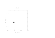
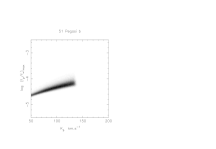
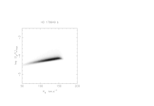
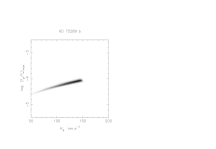
Figure 2: Prior probability density maps for the planet/star flux ratio near superior conjunction, as a function of the planet’s projected orbital velocity $K_{p}$, for an assumed geometric albedo $p=0.4$. The maps are calculated for an evolutionary radius model that exhibits a “Hot” atmospheric structure, although maximum likelihood values for both the “Hot” and “Cold” scenarios are shown at Table 3. Trials in which the orbital inclination was high enough to cross the observer’s line of sight to the stellar disc were rejected for all cases bar HD 209458 b, since none of these other systems has been seen to exhibit transits [Henry et al.2000a, Tinney et al.2001]. For the transiting planet, its known inclination and mass act to constrain the projected radial velocity amplitude. In the case of $\tau Bootis$, an additional constraint was applied. Since the rotation of the primary appears to have become synchronised with the planet’s orbit [Baliunas et al.1997, Collier Cameron et al.1999, Henry et al.2000a], the planet must have been massive enough to have synchronised the star’s spin within its own main sequence lifetime. For each trial we computed both the main sequence lifetime and the synchronisation timescale. Trials in which the latter exceeded the former were rejected. This, in conjunction with the well determined $v\sin{i}$ value, leads to a fairly tight constraint on the system inclination and hence $K_{p}$.

Planet	$K_{p}$	Inclination	$M_{p}/M_{Jup}$	$(f_{p}/f_{*})_{max}$	$(f_{p}/f_{*})_{max}$
	($km.s^{-1}$)	(Degrees)		Hot model	Cold Model
$\upsilon$ And b	133	78	0.760	4.88 x $10^{-5}$	4.53 x $10^{-5}$
$\tau$ Boo b	95	37	6.813	4.18 x $10^{-5}$	3.22 x $10^{-5}$
51 Peg b	117	63	0.523	4.81 x $10^{-5}$	4.46 x $10^{-5}$
HD 179949 b	135	60	0.945	6.44 x $10^{-5}$	5.34 x $10^{-5}$
HD 75289 b	141	75	0.498	7.38 x $10^{-5}$	9.17 x $10^{-5}$
HD 209458 b	144	87	0.620	7.18 x $10^{-5}$	7.17 x $10^{-5}$

Table 3: Maximum likelihood statistics for the parameter distributions returned by the Monte Carlo trials, given what we already know about the system from observation. In adopting a grey albedo of $p=0.4$ for our trials, similar to that of the Class V models of sudarsky2000. In reality, we would expect the albedo spectra of Pegasi planets to exhibit a strong wavelength dependence. However, we believe the use of a grey albedo spectra provides us with a realistic upper limit to the expected planet/star flux ratio.

For a Lambert-sphere phase function $g(\alpha)$ we can compute the maximum expected planet/star flux ratio near to superior conjunction,

$$(f_{p}/f_{*})_{max}=pg(\pi/2-i)\left(\frac{R_{p}}{a}\right)^{2}.$$ (6)

We adopt the Lambert-sphere phase function because it provides a good approximation to the phase functions of gas giants within our own solar system [Pollack et al.1986, Charbonneau et al.1999]. Although we expect the albedo spectra of Pegasi planets to exhibit a strong wavelength dependence, here we adopt a simple grey geometric albedo $p=0.4$ as a plausible comparison to the case of a high, reflective silicate cloud deck with little overlying absorption, as in the Class V models of sudarsky2000. Other models in which cloud layers are deeper, or even absent, produce lower optical albedos; thus the flux ratios we compute here should be treated as upper limits on the plausible planet/star flux ratio.

4 Method Limitations

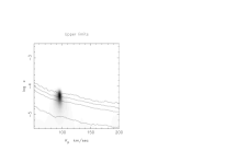
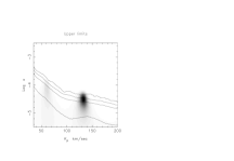
Figure 3: Results from reflected-light studies of (a) $\tau$ Bootis [Leigh et al.2003] and (b) $\upsilon$ Andromeda [Collier Cameron et al.2002], shown as relative probability maps of model parameters $K_{p}$ and $\log(\epsilon_{0})=\log p(R_{p}/a)^{2}$. The results are derived from WHT/UES observations of $\tau$ Bootis and $\upsilon$ Andromeda, assuming a grey albedo spectrum. The greyscale denotes the probability relative to the best-fit model, increasing from 0 for white to 1 for black. The contours show the confidence levels at which candidate detections can be ruled out as being caused by spurious alignments of non-Gaussian noise features. From top to bottom, they show the 99.9%, 99.0%, 95.4% and 68.3% confidence limits. The dark features in each probability map represent candidate planetary detections from the data but occur at too low a confidence level to guarantee a genuine detection. We note, however, that in both cases the main features appear close to the $K_{p}$ values predicted at Table 3 by Monte Carlo simulations and shown at Figure 2.

Target	$m_{V}$	$(f_{p}/f_{*})_{max}$	4m-class	8m-class
	(Mags)	Hot model	telescopes	telescopes
$\upsilon$ And	4.09	4.88 x $10^{-5}$	20.0 hrs	5.0 hrs
$\tau$ Boo	4.50	4.18 x $10^{-5}$	39.8 hrs	9.9 hrs
51 Peg	5.46	4.81 x $10^{-5}$	72.7 hrs	18.2 hrs
HD 179949	6.25	6.44 x $10^{-5}$	84.0 hrs	21.0 hrs
HD 75289	6.35	7.38 x $10^{-5}$	70.1 hrs	17.5 hrs
HD 209458	7.65	7.18 x $10^{-5}$	245 hrs	61.3 hrs

Table 4: Exposure time predictor to compare benefits of observing different star and telescope class combinations. We take 4m-class observations on $\upsilon$ Andromeda as our standard, with an exposure time benchmark of 20.0 hrs required to reach the predicted $(f_{p}/f_{*})_{max}$ signal levels. In deriving these estimates we assume that all other variables are equal, such as overall instrument efficiency, observing strategies and weather conditions.

Spectroscopic reflected-light searches should provide us with a unique opportunity to achieve the direct detection of a Pegasi planet, however there exist a number of potential difficulties that require a cautious approach to any analysis.

(i) At the flux ratios we are working ($f_{p}/f_{*}<10^{-4}$), we inevitably see the appearence of systematic non-gaussian noise within data sets, noise that requires to be carefully identified and corrected for in the subsequent analysis.

(ii) Any predictions from our searches require assumptions to be made about the nature of the planetary system, such as the phase function $g(\alpha,\lambda)$, the planetary radius $R_{p}$ or albedo spectra $p(\lambda)$, and that the orbital and stellar equatorial planes are co-aligned. To some extent observational results will therefore act to narrow the range of parameter space occupied by these Pegasi planets, although stronger detections will allow us to draw more definite conclusions.

(iii) The “Doppler Wobble” method of detection confirms the existence of a planet but cannot tell us its true orbital inclination. A spectroscopic search for the reflected-light component of a close orbiting planet has the potential to identify the projected orbital velocity $K_{p}$ and hence the orbital tilt. However, with such a scope of possible $K_{p}$ values, it is important to estimate where we might expect to detect the planet, given the known parameters of the system. Such estimates, as detailed in Section 5, provide us with a quantifiable method by which we can assess the plausibility of any candidate detection.

5 Probability Distributions

We derive the prior probability distributions for the observable quantities $K_{p}$ and $(f_{p}/f_{*})_{max}$ by drawing randomly from the uncertainty distributions (assumed gaussian) for the observed quantities $K_{*}$, $M_{*}$, $R_{*}$, $P_{rot}$, Age and $v\sin{i}$. The values of these quantities, for 6 of the brightest stars known to harbour Pegasi planets with orbital periods of less than 5 days, are given in Tables 1 and 2. In order to provide a radius estimate for each planet $R_{p}$, we use our $\sin i$ estimate to conduct a $\log{R_{p}}-\log{M_{p}}$ linear interpolation (for a selected Age) between the $\sin i=1.0$ and $\sin i=0.5$ evolutionary models. This is done for both the “Hot” and “Cold” evolutionary scenarios. In each case we performed 1,000,000 random Monte Carlo trials to compute $K_{p}$ and $\log(f_{p}/f_{*})_{max}$. The resulting joint probability distributions for the planet/star flux ratio and projected orbital velocity amplitude are presented in Figure 2.

6 Discussion

The maximum observable planet/star flux ratio for a planet depends strongly on the inclination of its orbit to our line of sight, and on the distance of the planet from the star. The statistical analyses presented here provide estimates of the planet/star flux ratio, derived from the best data currently available on 6 bright stars harbouring planets with orbital periods of less than 5 days. These estimates are model-dependent, in that we have made theoretical assumptions about each planet’s radius, the co-alignment of each orbital plane to the stellar rotation axis and used a Lambert-sphere phase function to describe the atmospheric scattering properties. In addition, we have adopted a grey geometric albedo $(p=0.4)$ that corresponds roughly to the reflective, high-level silicate cloud decks predicted by the Class V spectral models of sudarsky2000.

Recent spectroscopic searches for relected-light signatures from $\tau$ Bootis b [Leigh et al.2003] and $\upsilon$ Andromeda b [Collier Cameron et al.2002], shown at Figure 3, have already reached detection limits comparable to the signal levels predicted here, using echelle spectrographs on 4m-class telescopes. We find the total number of photons that must be collected scales with the square of the planet/star flux ratio, whilst the length of time required to collect this number of photons with a given telescope scales with the flux received from the star. If we adopt 4m-class observations of $\upsilon$ Andromeda as our benchmark (20.0 hrs) to reach the $(f_{p}/f_{*})_{max}$ signal levels predicted, then Table 4 details the relative exposure times for each planetary system, given access to both 4m and 8m-class telescope facilities. Given that it has been possible to probe to these deep signal levels for $\upsilon$ And in only a few nights on a 4m-class telescope, the remaining 5 targets are clearly viable and compelling targets for future studies with existing high-throughput spectrographs on 8m-class telescopes. Future instruments that are also likely to be useful in this respect include the high-efficiency fibre-fed echelle spectrograph ESPADONS, which is to be commissioned on CFHT during 2003.

References

- [\citefmtBaliunas et al.1997] Baliunas S., Henry G., Donahue R., Fekel F., Soon W., 1997, ApJ, 474, 119
- [\citefmtBaraffe et al.2003] Baraffe I., Chabrier G., Barman T., Allard F., Hauschildt P., 2003, Astronomy and Astrophysics, 402, 701
- [\citefmtBarman, Hauschildt & Allard2001] Barman T., Hauschildt P., Allard F., 2001, ApJ, 556, 885
- [\citefmtBarnes2001] Barnes S., 2001, ApJ, 561, 1095
- [\citefmtBenz & Mayor1984] Benz W., Mayor M., 1984, Astronomy and Astrophysics, 138, 183
- [\citefmtBodenheimer, Lin & Mardling2001] Bodenheimer P., Lin D., Mardling R., 2001, ApJ, 548, 466
- [\citefmtBrown et al.2001] Brown T., Charbonneau D., Gilliland R., Noyes R., Burrows A., 2001, ApJ, 552, 699
- [\citefmtBurrows et al.1997] Burrows A., Marley M., Hubbard W., Sudarsky D., Guillot T., 1997, ApJ, 491, 856
- [\citefmtBurrows et al.2000] Burrows A., Guillot T., Hubbard W., M. M., Saumon D., Lunine J., Sudarsky D., 2000, ApJ, 534, 97
- [\citefmtBurrows, Sudarsky & Hubbard2003] Burrows A., Sudarsky D., Hubbard W., 2003, ApJ, In press : astro-ph/0305277
- [\citefmtButler et al.1997] Butler P., Marcy G., Williams E., Hauser H., Shirts P., 1997, ApJ, 474, 115
- [\citefmtCharbonneau et al.1999] Charbonneau C., Noyes D., Jha S., Vogt S., 1999, ApJ, 522, 145
- [\citefmtCharbonneau et al.2000] Charbonneau D., Brown T., Latham D., Mayor M., 2000, ApJ, 529, 45
- [\citefmtCho et al.2003] Cho J., Menou K., Hansen B., Seager S., 2003, ApJ, 587, 117
- [\citefmtCody & Sasselov2002] Cody A., Sasselov D., 2002, ApJ, 569, 451
- [\citefmtCollier Cameron et al.1999] Collier Cameron A., Horne K., Penny A., James D., 1999, Nat, 402, 751
- [\citefmtCollier Cameron et al.2002] Collier Cameron A., Horne K., Penny A., Leigh C., 2002, MNRAS, 330, 187
- [\citefmtFuhrmann, Pfeiffer & Bernkopf1997] Fuhrmann K., Pfeiffer J., Bernkopf J., 1997, Astronomy and Astrophysics, 326, 1081
- [\citefmtFuhrmann, Pfeiffer & Bernkopf1998] Fuhrmann K., Pfeiffer J., Bernkopf J., 1998, Astronomy and Astrophysics, 336, 942
- [\citefmtGonzalez & Laws2000] Gonzalez G., Laws C., 2000, AJ, 119, 390
- [\citefmtGonzalez et al.2001] Gonzalez G., Laws C., Tyagi S., Reddy B., 2001, AJ, 121, 432
- [\citefmtGonzalez1998] Gonzalez G., 1998, Astronomy and Astrophysics, 334, 221
- [\citefmtGoukenleuque, Bezard & Lellouch1999] Goukenleuque C., Bezard B., Lellouch E., 1999, DPS (AAS) Conf., 31, 0906G
- [\citefmtGratton, Focardi & Bandiera1989] Gratton R., Focardi P., Bandiera R., 1989, MNRAS, 237, 1085
- [\citefmtGray, Napier & Winkler2001] Gray R., Napier M., Winkler L., 2001, AJ, 121, 2148
- [\citefmtGray1992] Gray D., 1992, The Observation and Analysis of Stellar Photospheres. Cambridge University Press, Cambridge, U.K
- [\citefmtGroot, Piters & van Paradijs1996] Groot P., Piters A., van Paradijs J., 1996, A&AS, 118, 545
- [\citefmtGuillot & Showman2002] Guillot T., Showman P., 2002, Astronomy and Astrophysics, 385, 156
- [\citefmtGuillot et al.1996] Guillot T., Burrows A., Hubbard W., Lunine J., Saumon D., 1996, ApJ, 459, 35
- [\citefmtGuillot1999] Guillot T., 1999, Sci, 286, 72
- [\citefmtHenry et al.2000a] Henry G., Baliunas S., Donahue R., Fekel F., Soon W., 2000a, ApJ, 531, 415
- [\citefmtHenry et al.2000b] Henry G., Marcy G., Butler P., Vogt S., 2000b, ApJ, 529, 41
- [\citefmtHouk & Smith-Moore1988] Houk N., Smith-Moore M., 1988, MSS, C04, 0H
- [\citefmtLeigh et al.2003] Leigh C., Collier Cameron A., Horne K., Penny A., James D., 2003, MNRAS, MNRAS accepted, astro-ph/0308413
- [\citefmtMarcy et al.1997] Marcy G., Butler P., Williams E., Bildsten L., Graham J., Ghez A., Jernigan G., 1997, ApJ, 481, 926
- [\citefmtMarley, Gelino & Stephens1999] Marley M., Gelino C., Stephens D., 1999, ApJ, 513, 879
- [\citefmtMayor & Queloz1995] Mayor M., Queloz D., 1995, Nat, 378, 355
- [\citefmtMazeh et al.2000] Mazeh T., Naef D., Torres G., Latham D., Mayor M., 2000, ApJ, 532, 55
- [\citefmtPollack et al.1986] Pollack J., Rages K., Baines K., Bergstrahl J., 1986, Icarus, 65, 442
- [\citefmtQueloz et al.2000] Queloz D., Eggenberger A., Mayor M., Perrier C., Beuzit J., 2000, Astronomy and Astrophysics, 359, 13
- [\citefmtSeager & Sasselov1998] Seager S., Sasselov D., 1998, ApJ, 502, 157
- [\citefmtShowman & Guillot2002] Showman P., Guillot T., 2002, Astronomy and Astrophysics, 385, 166
- [\citefmtSudarsky, Burrows & Hubeny2003] Sudarsky D., Burrows A., Hubeny I., 2003, ApJ, 588, 1121
- [\citefmtSudarsky, Burrows & Pinto2000] Sudarsky D., Burrows A., Pinto P., 2000, ApJ, 538, 885
- [\citefmtTinney et al.2001] Tinney C., Butler R., Marcy G., Jones H., Penny A., Vogt S., 2001, ApJ, 551, 507
- [\citefmtUdry et al.2000] Udry S., Mayor M., Naef D., Pepe F., Queloz D., Santos N., 2000, Astronomy and Astrophysics, 356, 590