A new upper limit on the reflected starlight from $\tau$ Bootis $b$

Abstract

Using improved doppler tomographic signal-analysis techniques we have carried out a deep search for starlight reflected from the giant planet orbiting the star $\tau$ Bootis. We combined echelle spectra secured at the 4.2 m William Herschel telescope in 1998 and 1999 (which yielded a tentative detection of a reflected starlight component from the orbiting companion) with new data obtained in 2000 (which failed to confirm the detection). The combined dataset comprises 893 high resolution spectra with a total integration time of $75^{hr}32^{min}$ spanning 17 nights. We establish an upper limit on the planet’s geometric albedo $p<0.39$ (at the 99.9% significance level) at the most probable orbital inclination $i\simeq 36^{\circ}$, assuming a grey albedo, a Venus-like phase function and a planetary radius $R_{p}=1.2R_{Jup}$. We are able to rule out some combinations of the predicted planetary radius and atmospheric albedo models with high, reflective cloud decks. Although a weak candidate signal appears near to the most probable radial velocity amplitude, its statistical significance is insufficient for us to claim a detection with any confidence.

Key Words: Planets: extra-solar - Planets: atmosphere - Stars: $\tau$ Bootis

1 Introduction

Two years after the discovery of a planetary companion to 51 Pegasi by mayor95 came the identification of a similar object orbiting the F7V star $\tau$ Bootis [Butler et al.1997]. Among the more surprising features of these discoveries were their short orbital periods, putting both objects very close to their parent stars. Indeed, of the 102 extra-solar planets currently known, 19 reside within 0.1 AU of the parent star. In addition to posing many theoretical questions as to how they came to be there, the existence of these objects in such close orbits does open the possibility of their detection through the reflection of the host stellar spectrum.

Shortly after the $\tau$ Bootis b detection, two teams [Charbonneau et al.1999, Cameron et al.1999] initiated a spectroscopic search for the reflected light component of the orbiting planet. Charbonneau et al. conducted 3 nights observation in March 1997 using the HIRES echelle spectrograph mounted on the Keck I 10m telescope on Mauna Kea, Hawaii. Although the restricted spectral range 465.8 - 498.7 nm provided a non detection, the signal-to-noise ratio ($SNR\sim 1500$) was sufficient to impose a relative reflected flux limit $f_{p}/f_{*}<5\times 10^{-5}$, assuming a grey albedo reflection of the stellar spectrum. This implies a geometric albedo limit $p<0.3$ over the spectral range investigated, assuming a planetary radius of $1.2~{}R_{Jupiter}$. Cameron et al. obtained 10 nights of data during 1998 and 1999, with the Utrecht echelle spectrograph (UES) on the 4.2 m William Herschel telescope. By using a least-squares deconvolution (LSD) technique [Donati et al.1997] on $\sim 2300$ spectral lines in the range 385 - 611 nm, they identified a probable reflected-light feature with $f_{p}/f_{*}\sim 7.8\times 10^{-5}$ [Cameron et al.1999]. This detection indicated an orbital velocity amplitude $K_{p}=74\pm 3$ km s^-1 which, when combined with the planet’s orbital velocity $V_{p}=152$ km s^-1, suggested an inclination for the system $i=29^{o}$ and a radius $R_{p}=1.8R_{J}$, assuming a grey geometric albedo $p=0.55$. A bootstrap Monte Carlo analysis gave a 5% probability that the feature was an artefact of noise. Subsequent observations over 7 nights in March-May 2000, however, failed to confirm the detection [Collier Cameron et al.2001].

Table 1: System parameters for $\tau$ Bootis and its planetary companion

Parameter	Value (Uncertainty)	References
$\bf{Star:}$
Spectral Type	F7V	fuhrmann98,gonzalez98
$M_{V}$	4.496 (0.008)	fuhrmann98,gonzalez98
Distance (pc)	15.6 (0.17)	perryman97
$T_{Eff}$ (K)	6360 (80)	fuhrmann98,gonzalez98
$M_{*}(M_{\odot})$	1.42 (0.05)	fuhrmann98,gonzalez98
$R_{*}(R_{\odot})$	1.48 (0.05)	fuhrmann98,gonzalez98
$\left[Fe/H\right]$	0.27 (0.08)	fuhrmann98,gonzalez98
v$\sin i$ (km s-1)	14.9 (0.5)	henry2000
Age (Gyr)	1.0 (0.6)	fuhrmann98
$\bf{Planet:}$
Orbital Period $P_{orb}$ (days)	3.31245 (0.00003)	Marcy, private communication
Transit Epoch $T_{0}$ (JD)	2451653.968 (0.015)	Marcy, private communication
$K_{*}(ms^{-1})$	469 (5)	butler97
a (AU)	0.0489	butler97(revised for this paper)
$M_{P}\sin i(M_{Jup})$	4.38	butler97(revised for this paper)

Here we report the results of a new, deep search for the reflected light signal via a full re-analysis of the WHT data, combining all 17 nights of echelle spectra obtained during the 1998, 1999 and 2000 observing seasons. In Section 2 we use the measured system parameters to determine prior probabilities for the planet’s orbital velocity amplitude and the fraction of the star’s light that it intercepts. In Section 3 and 4 we describe the acquisition and extraction of the echelle spectra. Section 5 details the methods used to extract the planetary signal from the data, by combining the profiles of thousands of stellar absorption lines recorded in each echellogram into a time series on which we use a matched-filter method to measure the strength of the reflected-light signal. Section 7 describes how we test and calibrate the analysis through the addition of a simulated planetary signal. Finally Section 8 makes theoretical assumptions about the size and atmospheric composition of $\tau$ Bootis b in order to place upper limits on its respective geometric albedo and radius. We also discuss the plausibility of a candidate reflected-light signature that appears in the data close to the most probable velocity amplitude and signal strength.

2 System Parameters

$\tau$ Bootis (HD 120136, HR 5185) is a late-F main sequence star with parameters as listed in Table 1. High precision radial velocity measurements over a period of 9 years were used to identify a planetary companion [Butler et al.1997] whose properties (as determined directly from the radial velocity studies or inferred using the estimated stellar parameters) are also summarised in Table 1.

The equations detailed below represent a summary of the more comprehensive derivations described in previous work [Cameron et al.1999, Charbonneau et al.1999, Cameron et al.2002].

As the planet orbits its host star, some of the starlight incident upon its surface is reflected towards us, producing a detectable signature within the observed spectra of the star. This signature takes the form of faint copies of the stellar absorption lines, Doppler shifted due to the planet’s orbital motion and greatly reduced in intensity ($\sim 10^{-4}$) due to the small fraction of starlight the planet intercepts and reflects back into space.

With our knowledge of stellar mass and the planet’s orbital period we can estimate the orbital velocity of the planet $V_{p}$. The apparent radial velocity amplitude $K_{p}$ of the reflected light is given by:

$$K_{p}=V_{p}\sin i=161\sin i~{}\mbox{km~{}s}^{-1}$$ (1)

where the orbital inclination $i$ is, according to the usual convention, the angle between the orbital angular momentum vector and the line of sight.

For all but the lowest inclinations, the orbital velocity amplitude of the planet is substantially greater than the broadened widths of the photospheric absorption lines of the star. Hence, lines in the reflected-light spectrum of the planet should be Doppler shifted well clear of their stellar counterparts, allowing a clean spectral separation for most of the orbit.

By isolating the reflected planetary signature, we are in effect observing the planet/star flux ratio ($\epsilon$) as a function of orbital phase ($\phi$) and wavelength ($\lambda$).

$$\epsilon(\alpha,\lambda)\equiv\frac{f_{p}(\alpha,\lambda)}{f_{\star}(\lambda)}=p(\lambda)g(\alpha,\lambda)\frac{R_{p}^{2}}{a^{2}}=\epsilon_{0}(\lambda)g(\alpha,\lambda)$$ (2)

The phase function $g(\alpha,\lambda)$ describes the variation in the star-planet flux ratio with illumination phase angle $\alpha$. This is the angle subtended at the planet by the star and the observer, and varies according to $\cos\alpha=-\sin i.\cos\phi$.

The observations measure $\epsilon(\alpha,\lambda)$ over some range of orbital phases $\phi$ and hence phase angles $\alpha$. However, the signal-to-noise ratio and orbital phase coverage of the observations is not yet adequate to define the shape of the phase function. Accordingly, current practice is to adopt a specific phase function in order to express the results in terms of the planet/star flux ratio that would be seen at phase angle zero:

$$\epsilon_{0}(\lambda)=p(\lambda)\frac{R_{p}^{2}}{a^{2}}$$ (3)

where $p(\lambda)$ is the wavelength dependent geometric albedo. Since $a$ is tightly constrained by Kepler’s third law to $a=0.0489\left(M_{*}/1.42M_{\odot}\right)~{}AU$, the measurements of $\epsilon_{0}(\lambda)$ measure the product $R_{p}\sqrt{p(\lambda)}$.

While the phase function of a Lambert sphere might be the simplest form to adopt for $g(\alpha,\lambda)$, we prefer to adopt a phase function that resembles those for the cloud-covered surfaces of planets in our own solar system. Jupiter and Venus appear to have phase functions that are more strongly back-scattering than a Lambert sphere. Photometric studies of Jupiter at large phase angles from the Pioneer and subsequent missions have shown [Hovenier1989] that the phase function for Jupiter is very similar to that of Venus, despite their very different cloud compositions. As a plausible alternative to the Lambert-sphere formulation, we use a polynomial approximation to the empirically determined phase function for Venus [Hilton1992]. The phase-dependent correction to the planet’s visual magnitude is approximated by:

$$\Delta m(\alpha)=0.09(\alpha/100^{\circ})+2.39(\alpha/100^{\circ})^{2}-0.65(\alpha/100^{\circ})^{3}$$ (4)

so that

$$g(\alpha)=10^{-0.4\Delta m(\alpha)}$$ (5)

In the event of any planetary detection, a careful analysis of the data should allow us to determine the following information:

(i) $K_{P}$, the planet’s projected orbital velocity, from which we obtain the orbital inclination of the system and hence the mass of the planet, since $M_{P}\sin i$ is known from the star’s Doppler wobble.

(ii) $\epsilon_{0}$, the maximum flux ratio observed, with which we can constrain the planet’s radius since $\epsilon_{0}=p(R_{P}/a)^{2}$, where $p$ is the geometric albedo of the planetary atmosphere. Alternatively we can adopt a theoretical radius to constrain the albedo of a given atmospheric model.

2.1 Rotational broadening

The rotational broadening of the direct starlight and chromospheric Ca II H & K emission flux suggest that the star’s rotation is synchronised with the orbit of the planet [Baliunas et al.1997, Henry et al.2000]. In a tidally locked system there is no relative motion between the surface of the planet and the surface of the star, so the planet will reflect a non-rotationally broadened stellar spectrum, with typical line widths dominated by turbulent velocity fields in the stellar photosphere. These motions were estimated by baliunas97 to be of the order $\sim 4$ km s^-1. Any absorption lines attributed to the planet’s atmosphere are thus likely to be much narrower than the stellar lines.

2.2 Orbital Inclination

In the first instance we can rule out inclinations $i>80^{\circ}$ due to the absence of transits in high-precision photometry [Henry et al.2000]. Furthermore, if we assume the star’s rotation to be tidally locked to the planet’s orbit, we can use the projected equatorial rotation speed of the host star $v\sin i=14.9\pm 0.5$ km s^-1 [Henry et al.2000] to loosely constrain the orbital inclination to $i\sim 40^{\circ}$. We would thus expect a projected orbital velocity amplitude close to $K_{p}\sim 100$ km s^-1.

2.3 Planet Radius

The HD 209458b transit detection of charb2000 provided the first confirmation of the gas giant nature of close-in extra solar planets, and yielded a radius in good agreement with the predictions of past and current interior structure models [Guillot et al.1996, Seager & Sasselov1998, Marley, Gelino & Stephens1999, Burrows et al.2000, Seager, Whitney & Sasselov2000]. In short, the planet radius evolves with time and depends on the planet mass. For our purposes, this defines a range of theoretically plausible radii at each possible value of the planet mass. The range of possible planet radii was computed specifically for $\tau$ Bootis b by burrows2000, allowing for uncertainties in the orbital inclination and hence the planet’s mass. Their radiative-convective gas giant models predict upper limits on the planet’s radius of 1.58 $R_{Jup}$ for $M_{p}$ = 7 $M_{Jup}$, and 1.48 $R_{Jup}$ for $M_{p}$ = 10 $M_{Jup}$.

2.4 Prior Estimates of System Parameters

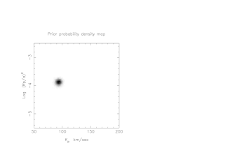
Figure 1: The greyscale shows the prior joint probability density function (PDF) for projected orbital velocity $K_{p}$ and the squared ratio $(R_{p}/a)^{2}$ of the planet radius to the orbit radius, based on the measured system parameters. Darker shades in the greyscale denote greater probabilities of the planet having the corresponding combination of $(R_{p}/a)^{2}$ and $K_{p}$. The PDF shows that the planet is most likely to have $K_{p}\simeq 94$ km s^-1 and $(R_{p}/a)^{2}\simeq 1.44\times 10^{-4}$.

Table 2: Journal of observations. The UTC mid-times and orbital phases are shown for the first and last spectral exposures secured on each night of observation. The number of exposures is given in the final column.

UTC start	Phase	UTC End	Phase	Exposures
1998 Apr 09 22:09:43	0.425	1998 Apr 10 05:37:05	0.519	107
1998 Apr 10 22:04:40	0.726	1998 Apr 11 06:20:54	0.830	113
1998 Apr 11 22:09:28	0.029	1998 Apr 12 05:58:44	0.127	81
1998 Apr 13 23:02:54	0.644	1998 Apr 14 05:37:05	0.733	33
1999 Apr 02 22:06:45	0.493	1999 Apr 03 06:08:47	0.594	25
1999 Apr 25 21:43:17	0.441	1999 Apr 26 05:31:59	0.539	40
1999 May 05 21:56:59	0.463	1999 May 06 04:51:57	0.550	60
1999 May 25 20:59:45	0.488	1999 May 26 03:56:18	0.576	51
1999 May 28 20:52:23	0.390	1999 May 29 03:04:35	0.467	47
1999 Jun 04 20:22:34	0.497	1999 Jun 05 00:07:23	0.548	23
2000 Mar 14 23:14:49	0.271	2000 Mar 15 06:54:52	0.366	48
2000 Mar 15 22:51:55	0.567	2000 Mar 16 06:49:04	0.669	45
2000 Mar 24 22:21:55	0.278	2000 Mar 25 06:47:50	0.385	34
2000 Apr 23 20:38:59	0.311	2000 Apr 24 05:07:31	0.420	45
2000 Apr 24 20:58:32	0.619	2000 Apr 25 05:14:11	0.724	57
2000 May 13 20:47:01	0.349	2000 May 14 03:12:08	0.434	41
2000 May 17 20:24:14	0.557	2000 May 18 03:52:37	0.649	43

In searching for a faint reflected-light signature from a planet with an unknown orbital inclination, it is useful to know in advance how the planet’s observable properties ought to depend on the orbital inclination. We do this by constructing the a priori probability density functions for the various observable properties of the planet described in Table 1. This helps us to determine whether any faint candidate reflection signature is physically plausible, given our existing knowledge of the system’s parameters. We do not want to be guided too closely by theory, but values outside the plausible ranges would pose difficulties for current thinking.

Fig. 1 shows the probability distributions for the planet’s radial velocity amplitude $K_{p}$ and the quantity $(R_{p}/a)^{2}$, based on a Monte Carlo simulation using the expressions given in Section 2. We assume Gaussian distributions for the measured stellar mass ($1.42\pm 0.05M_{\odot}$), radius ($1.48\pm 0.05R_{\odot}$), stellar reflex velocity ($469\pm 5$ m s^-1) and the radius of the planet. The planet radius and uncertainty range were obtained from the theoretical mass-radius relations [Guillot et al.1996, Burrows et al.2000] described above. Both works find the most probable radius to be $1.2\pm 0.1R_{Jup}$, assuming $\tau$ Bootis b to have an age of 1 Gyr.

Furthermore, we assume the star’s rotation is tidally locked to the planet’s orbit. We thus generate a distribution of $\sin i$ values based on Gaussian distributions for the projected stellar rotation speed ($v\sin i=14.9\pm 0.5$ km s^-1) and a stellar rotation period (3.3 $\pm$ 0.1 days) closely bound to the orbital period of the planet. A further restriction applies where the tidal synchronisation timescale for the primary’s rotation,

$$\tau_{sync}\simeq 1.2\left(\frac{M_{p}}{M_{*}}\right)^{-2}\left(\frac{a}{R_{*}}\right)^{6}~{}years$$ (6)

is longer than the main-sequence liftime of the host star $\tau_{ms}\simeq 10^{10}(M_{*}/M_{\odot})^{-3}$ years, in which case we reject that model from the Monte Carlo analysis.

The resulting probability map (Fig. 1) shows a $K_{p}$ distribution centred on $\simeq 94$ km s^-1, with the most likely value of $(R_{p}/a)^{2}~{}\simeq 1.44\times 10^{-4}$. The projection of this PDF on to the orbital velocity axis defines the region of parameter space in which we can be confident that a detection would occur if it were present in the data, given our prior knowledge of the system parameters. We use the $K_{p}$ projection of the PDF in the subsequent analysis to test the plausibility of any candidate features which appear in the data, by modifying the posterior probability distribution to assess the false alarm probability (see Section 8.2.1). Secondly, our upper limits on $\epsilon_{0}$ are sensitive to the orbital inclination, so we adopt the most probable $K_{p}$ in order to determine the most plausible upper limits on the planet’s radius and albedo.

For any given albedo model we can also use the data to determine upper limits on $(R_{p}/a)^{2}$ instead of the opposition flux ratio $\epsilon_{0}$. The projection of the PDF onto $(R_{p}/a)^{2}$ thus allows us to compare the effective reflection area of the planet directly with model predictions. Unlike the projection on to $K_{p}$, however, the prior probability distribution for $(R_{p}/a)^{2}$ plays no role in assessing the plausibility or otherwise of a candidate detection.

3 Observations

We observed $\tau$ Bootis during 1998, 1999 and 2000 using the Utrecht Echelle Spectrograph on the 4.2 m William Herschel Telescope at the Roque de los Muchachos Observatory on La Palma. The detector was a single SITe 1 CCD array containing some $2048\times 2048$ 13.5-$\mu$m pixels. The CCD was centred at 459.6 nm in order 124 of the 31 g mm^-1 echelle grating, giving complete wavelength coverage from 407.4 nm to 649.0 nm with minimal vignetting. The average pixel spacing was close to 3.0 km s^-1, and the full width at half maximum intensity of the thorium-argon arc calibration spectra was 3.5 pixels, giving an effective resolving power $R=53000$.

Table 2 lists the journal of observations for the 17 nights of data which contribute to the analysis presented in this paper. In the first year (1998) the stellar spectra were exposed between 100 and 200 seconds. For 1999 and 2000, the stellar spectra were exposed for between 300 and 500 seconds, depending upon seeing, in order to expose the CCD to a peak count of 40000 ADU per pixel in the brightest parts of the image. A 450-s exposure yielded about $1.2\times 10^{6}$ electrons per pixel step in wavelength in the brightest orders in typical (1 arcsec) seeing after extraction. We achieved this with the help of an autoguider procedure, which improves efficiency in good seeing by trailing the stellar image up and down the slit by $\pm 2$ arcsec during the exposure to accumulate the maximum S:N per frame attainable without risk of saturation. Note that the 450-s exposure time compares favourably with the 53-s readout time for the SITe 1 CCD in terms of observing efficiency – the fraction of the time spent collecting photons is above 90%. Following extraction, the S:N in the continuum of the brightest orders is typically 1000 per pixel.

4 Spectrum extraction

One-dimensional spectra were extracted from the CCD frames using an automated pipeline reduction system built around the Starlink ECHOMOP and FIGARO packages. Nightly flat-field frames were summed from 50 to 100 frames taken at the start and end of each night, using an algorithm that identified and rejected cosmic rays and other non-repeatable defects by comparing successive frames. Due to physical movement of the chip mounting between and during observation runs, it was found that the level of noise was reduced by the use of nightly flat fields rather than master flat fields for the entire year’s observations.

The initial tracing of the echelle orders on the CCD frames was performed manually on the spectrum of $\tau$ Bootis itself, using exposures taken for this purpose without dithering the star up and down the slit. The automated extraction procedure then subtracted the bias from each frame, cropped the frame, determined the form and location of the stellar profile on each image relative to the trace, subtracted a linear fit to the scattered-light background across the spatial profile, and performed an optimal (profile and inverse variance-weighted) extraction of the orders across the full spatial extent of the object-plus-sky region. Nightly flat-field balance factors were applied in the process using the 50 to 100 frames obtained at the start and end of each night of observations. In all, 55 orders ( orders 88 to 142 ) were extracted from each exposure, giving full spectral coverage from 407.4 to 649.1 nm with good overlap.

5 Extracting the planet signal

For a bright, cloudy model planet with $p=0.4$ and $R_{p}=1.2R_{Jup}$, we expect the flux of starlight scattered from the planet to be no more than one part in 18000 of the flux received directly from $\tau$ Bootis itself, even at opposition ($\alpha=0$). In order to detect the planet signal, we first subtract the direct stellar component from the observed spectrum, leaving the planet signal embedded in the residual noise pattern. A detailed description of this procedure is given in cameron02 Appendix A. The planet signal consists of faint Doppler-shifted copies of each of the stellar absorption lines. After cleaning up any correlated fixed-pattern noise remaining in the difference spectra (see cameron02 Appendix B), we then create a composite residual line profile, by fitting to the thousands of lines recorded in each echellogram (cameron02 Appendix C). Finally we use a matched-filter analysis (cameron02 Appendix D) to search for features in the time-series of composite residual profiles whose temporal variations in brightness and radial velocity resemble those of the expected reflected-light signature. For an assumed albedo spectrum $p(\lambda)$ and orbital velocity amplitude $K_{p}$, the fit of the matched filter to the data measures $(R_{p}/a)^{2}$.

6 Analysis Changes

In this new analysis of the $\tau$ Bootis data, we have made the following significant changes to the processing undertaken for the original cameron99 paper -

(i) The inclusion of the year 2000 data, which adds seven nights’ data taken at optimally-illuminated orbital phases to the analysis.

(ii) Full re-extraction of all three years’ data, again using optimal methods, and providing an increase in the spectral range by two echelle orders or $\sim$ 15 nm.

(iii) The use of nightly flat-field frames in the extraction routine, rather than the previous whole year flat-fields. Post extraction analysis showed a $\sim 4$% reduction in noise.

(iv) Increases in computational processing power over the intervening two years has allowed the analysis to be conducted on individual echelle frames, rather than having to co-add the spectra into groups of four prior to the deconvolution and matched-filter analysis.

(v) The inclusion of a Principal Component Analysis routine (PCA), as detailed in cameron02 Appendix B, to remove correlated fixed-pattern noise that was appearing in the difference spectra (i.e. raw spectra - stellar template frames).

(vi) The use of a more stringent calibration technique, described at Appendix A, to quantify and correct for the fraction of the planetary signal lost during the stellar subtraction, deconvolution and PCA routines. With this we produce shallower but more realistic upper limits than were stated by cameron2001, who assumed no loss of signal.

7 Simulated planet signatures

We verified that a faint planetary signal is preserved through the above sequence of operations in the presence of realistic noise levels, by adding a simulated planetary signal to the observed spectra. We also use the simulated signal to calibrate the strength of any detected signal (Appendix A). The simulations were based on the assumption that the planet’s rotation is close to being tidally locked, always keeping the same face towards the star. The resulting broadening of the spectral lines is therefore dominated by convective motions on the star’s surface, estimated at $\simeq 4$ km s^-1 [Baliunas et al.1997]. For our simulations we chose to use the slowly rotating giant star HR 5694, observed on several nights in 1999. HR 5694 is a F7III spectral type of similar temperature and elemental abundance to $\tau$ Bootis, but with an estimated $v\sin i\simeq 6.4\pm 1$ km s^-1, making it well suited to represent the reflected starlight [Baliunas et al.1997].

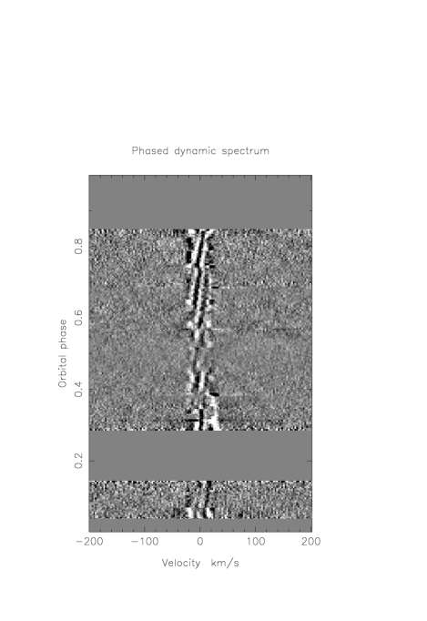
Figure 2: Time series of deconvolved profiles derived from the original WHT spectra, and secured over 17 nights observations in 1998, 1999 and 2000, but with the addition of a simulated planet signal at an inclination of $60^{\circ}$. The injected signal is that of a planet with geometric albedo $p=0.5$ and radius $1.4R_{Jup}$. The planetary signature appears as a dark sinusoidal feature crossing from right to left as phase increases and centred on the superior conjunction at phase 0.5.

Figure 3: Time series of deconvolved profiles derived from the original WHT spectra, and secured over 17 nights observations in 1998, 1999 and 2000. The observations assume a grey albedo spectrum without the addition of a synthetic planet signal. The greyscale runs from black at $-10^{-4}$ times the mean stellar continuum level, to white at $+10^{-4}$. The velocity scale is in the reference frame of the star.

For any assumed axial inclination, the phase angle and line-of-sight velocity are known at all times. The simulation procedure simply consists of shifting and scaling the spectrum of HR 5694 according to the orbit and phase function, co-multiplying it by an appropriate geometric albedo spectrum, and adding it to the observed data. To ensure a strong signal we used a simulated planet of radius 1.4 $R_{\rm Jup}$ and wavelength-independent geometric albedo $p=0.5$, which when viewed at zero phase angle should give a planet-to-star flux ratio $\epsilon_{0}=f_{p}/f_{*}=0.98\times 10^{-4}$. We have chosen a planetary radius greater than that expected by theory so as to provide a simulated input signal strong enough to return an unambiguous detection.

The resulting time series of deconvolved line profiles, shown in Fig. 2, demonstrates how the simulated planet signal is recovered after the extraction process, with the planetary signal clearly visible as a dark sinusoidal feature crossing from right to left between phases 0.25 and 0.75. The weakening of the simulated planetary signature near quadrature is caused mainly by the phase function. The signal is further attenuated near quadrature by the way in which the templates are computed: since the planet signature is nearly stationary in this part of the orbit, some of the signal will be removed along with the stellar profile if many observations are made in this part of the orbit.

Figure 4: Relative probability map of model parameters $K_{p}$ and $\log(\epsilon_{0})=\log p(R_{p}/a)^{2}$ for a simulated planet signature with grey albedo $p=0.5$, $R_{p}=1.4R_{Jup}$ and orbital inclination of 60 ^∘. The contours show the confidence levels at which candidate detections can be ruled out as being caused by spurious alignments of non-Gaussian noise features. From top to bottom, they show the 99.9%, 99.0%, 95.4% and 68.4% confidence limits. The synthetic planet signature is detected well above the 99.9% confidence limit.

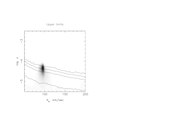
Figure 5: Relative probability map of model parameters $K_{p}$ and $\log(\epsilon_{0})=\log p(R_{p}/a)^{2}$, derived from the WHT/UES observations of $\tau$ Bootis, assuming a grey albedo spectrum. The greyscale denotes the probability relative to the best-fit model, increasing from 0 for white to 1 for black. A broad candidate feature appears close to the 99.0% confidence contour, with projected orbital velocity amplitude $K_{p}=97$ km s^-1.

Figure 6: The upper panel shows the optimal scaling factor $(R_{p}/a)^{2}$ plotted against orbital velocity amplitude $K_{p}$, assuming a grey albedo spectrum for the simulated planet data. The lower panel shows the associated reduction $\Delta\chi^{2}=84.6$, measured relative to the fit obtained in the absence of any planet signal i.e. for $(R_{p}/a)^{2}$ = 0. Note that only positive values of $(R_{p}/a)^{2}$ are physically plausible.

Figure 7: As for Fig. 6 but assuming a grey albedo spectrum for the original data without a simulated planet signal. The lower panel shows the associated reduction in $\Delta\chi^{2}=8.324$, measured relative to the fit obtained in the absence of any planet signal. The weak improvement in $\Delta\chi^{2}$ at $K_{p}=60$ km s^-1 corresponds to a negative value of $(R_{p}/a)^{2}$ and is therefore physically implausible.

Figs. 2 and 3 both show a “barber’s-pole” pattern of distortions in the residual stellar profiles at low velocities. The phase variation in these undulations appears consistent with sub-pixel shifts in the position of the spectra with respect to the detector over the course of the night. Fortunately they only affect a range of velocities at which the planet signature would in any case be indistinguishable from that of the star.

The relative probabilities of the fits to the data for different values of the free parameters $R_{p}/a$ and $K_{p}$ are given by

$$P(K_{p},R_{p}/a)\propto\exp(-\chi^{2}/2),$$ (7)

where

$$\chi^{2}=\sum_{i,j}\frac{(D_{ij}-(R_{p}/a)^{2}H(v_{i},\phi_{j},K_{p}))^{2}}{\sigma^{2}_{ij}}.$$ (8)

This is conveniently displayed in greyscale form as a function of $K_{p}$ and $\log(\epsilon_{0})=\log p(R_{p}/a)^{2}$. In Fig. 4 we show the map for the simulated observations, with the probabilities normalised to the most probable value in the map.

The signal of the synthetic planet appears as a compact, dark feature at $K_{p}=139$ km s^-1 and $\log(\epsilon_{0})=-4.01$, i.e. $\epsilon_{0}=0.98\times 10^{-4}$. This most probable combination of orbital velocity and planet radius yields an improvement $\Delta\chi^{2}=84.6$ with respect to the value obtained assuming no planet is present (Fig. 6).

To set an upper limit on the strength of the planet signal, or to assess the likelihood that a candidate detection is spurious, we need to compute the probability of obtaining such an improvement in $\chi^{2}$ by chance alone. In principle this could be done using the $\chi^{2}$ distribution for 2 degrees of freedom. In practice, however, the distribution of pixel values in the deconvolved difference profiles has extended non-Gaussian tails that demand a more cautious approach.

Rather than relying solely on formal variances derived from photon statistics, we use a “bootstrap” procedure to construct empirical distributions for confidence testing, using the data themselves. In each of 3000 trials, we randomize the order in which the 17 nights of observations were secured, then we randomise the order in which the observations were secured within each night. The re-ordered observations are then associated with the original sequence of dates and times. This ensures that any contiguous blocks of spectra containing similar systematic errors remain together, but appear at a new phase. Any genuine planet signal present in the data is, however, completely scrambled in phase. The re-ordered data are therefore as capable as the original data of producing spurious detections through chance alignments of blocks of systematic errors along a single sinusoidal path through the data. We record the least-squares estimates of $\log(\epsilon_{0})=\log p(R_{p}/a)^{2}$ and the associated values of $\chi^{2}$ as functions of $K_{p}$ in each trial.

The percentage points of the resulting bootstrap distribution are shown as contours in Figs. 4 and 5. From bottom to top, these contours give the 68.4%  95.4%  99.0% and 99.9% bootstrap upper limits on the strength of the planet signal. The 99.9% contour, for example, represents the value of $\log(\epsilon_{0})$ that was only exceeded in 3 of the 3000 trials at each $K_{p}$.

8 Results and Discussion

The results of this analysis appear on the relative probability map of model parameters $K_{p}$ and $\log(\epsilon_{0})=\log p(R_{p}/a)^{2}$, shown at Fig. 5. The calibrated confidence levels allow us to achieve our primary aim of constraining the radius and albedo of the planet. However, there exists a significant candidate feature close to the 99% level that requires further investigation. In the subsequent discussion, we therefore also explore the possibility that this feature could represent a genuine planetary detection.

If the feature were genuine, the projected orbital velocity amplitude $K_{p}\simeq 97~{}(\pm 10)~{}km~{}s^{-1}$ yields an orbital inclination of 37 ($\pm 5$)^∘. This would be consistent with the star’s rotation being tidally locked to the planet’s orbit and implies a mass for $\tau$ Bootis b of $M_{p}=7.28(\pm 0.83)M_{Jup}$.

We emphasise that, although the feature appears very close to the peak of the prior probability distribution projected onto $K_{p}$, shown in Fig. 1, there remains a distinct possibility that the candidate detection is a consequence of spurious noise and as such we should proceed with caution.

8.1 Upper Limits on Grey Albedo

The grey albedo model assumes that at all times the planet-star flux ratio is independent of wavelength. For an assumed planetary radius we can thus use Equation 3 to constrain the geometric albedo. Table 3 lists the upper limits on the albedo at various levels of significance, for the planetary radius $R_{p}=1.2R_{Jup}$ predicted by current theoretical models [Guillot et al.1996, Burrows et al.2000].

Table 3: Upper limits on the grey albedo for the atmosphere of $\tau$ Bootis b assuming a radius of 1.2 $R_{Jup}$. The upper limits are quoted for an assumed $K_{p}\simeq 94$ km s^-1, at the peak of the prior probability distribution for $K_{p}$.

False Alarm	$p\left(R_{p}/a\right)^{2}$	Upper Albedo Limit
Probability		$p$
0.1 %	0.561 E-04	0.39
1.0 %	0.403 E-04	0.28
4.6 %	0.305 E-04	0.21

The contours in Fig. 5 produced by the bootstrap simulation constrain the maximum reflected flux ratio at opposition to be $\epsilon_{0}\leq 0.561\times 10^{-4}$ at the 99.9 % confidence level, assuming a projected orbital velocity $K_{p}$ at the peak of the prior probability distribution, i.e. $K_{p}\simeq 94$ km s^-1. This would limit the geometric albedo of the planet to $p\leq 0.39$. We note that this is a similar result to that obtained by charb99 at the same inclination. Both studies assume a grey albedo, $R_{p}=1.2R_{Jup}$, synchronous rotation of the star and hence a reflected version of the stellar spectrum with no rotational broadening. The candidate feature that appears in Fig. 5 would, if genuine, yield a grey geometric albedo of $p~{}=~{}0.32~{}(\pm 0.13)$ for a planet of this radius.

8.2 Upper Limits on Radius

Figure 8: Geometric albedo spectra for the Class V (solid line), isolated (dashed) and irradiated (dot-dashed) Class IV models of sudarsky2000, plotted over the wavelength range we observed. Together with a grey model of albedo $p=0.3$, the Class V and isolated Class IV models were used to probe the wavelength dependence of candidate reflected-light signals. The geometric albedo spectrum of Jupiter (short dashes) is shown for comparison.

Here we investigate how atmospheric albedo models can be incorporated into the signal analysis to place upper limits on the size of the planet. A non-grey albedo model is built into the formation of the least-squares deconvolved profile, by scaling the strengths of the lines in the deconvolution mask by a factor equal to the geometric albedo at each line’s wavelength. The scale factor produced by the matched-filter analysis is then directly proportional to $(R_{p}/a)^{2}$ (see Equation 3) and is calibrated by injecting the signature of a planet of known radius with the specified albedo spectrum into the data. The method is described in detail by cameron02.

The theoretical models we consider here are those proposed by sudarsky2000 for a range of extrasolar giant planets, as shown at Fig. 8. These models are grouped primarily by their mass and orbital distance from the host star, factors which in turn influence their effective surface temperature, surface gravity and hence radius. We recognise, however, that recent observations of the atmosphere of HD 209458b [Charbonneau et al.2002] suggest there may be less sodium absorption than predicted in these and other models [Brown et al.2001, Hubbard et al.2001].

Table 4: Upper limits on planet radius for various albedo models. The limits are quoted for an assumed $K_{p}\simeq 94$ km s^-1, at the peak of the prior probability distribution for $K_{p}$. Note that the results for the grey albedo model are given for a geometric albedo of $p=0.3$. Radii for other grey model albedos can be obtained by dividing Column 4 by $\sqrt{p/0.3}$ .

Albedo Model	False Alarm	$(R_{p}/a)^{2}$	$R_{p}/R_{Jup}$
	Probability		Upper Limit
Grey	0.1%	1.87 E-04	1.37
($p=0.3$)	1.0%	1.34 E-04	1.16
	4.6%	1.02 E-04	1.01
Class V	0.1%	1.16 E-04	1.08
	1.0%	0.91 E-04	0.95
	4.6%	0.63 E-04	0.79
Class IV	0.1%	1.50 E-04	1.22
(Isolated)	1.0%	1.13 E-04	1.06
	4.6%	0.87 E-04	0.93

Table 5: Projected orbital velocity peak, planet radius, $\Delta\chi^{2}$ and false-alarm probabilities (FAP) for the candidate feature, on the basis that it represents a genuine detection.The second FAP weights $K_{p}$ in proportion to the prior probability density distribution (Fig. 1).

Albedo Model	$K_{p}$	$R_{p}/R_{Jup}$	$\Delta\chi^{2}$	FAP	FAP
	($km~{}s^{-1}$)			(Uniform Weight)	($K_{p}$ Prior)
Grey ($p=0.3$)	97 ($\pm 8$)	$1.24\pm 0.25$	8.324	0.147	0.036
Class V	95 ($\pm 8$)	$1.08\pm 0.19$	12.06	0.032	0.003
Class IV	90 ($\pm 8$)	$1.18\pm 0.20$	9.227	0.092	0.032

8.2.1 Grey Albedo Model

At the most probable values in the prior distribution ($K_{p}\simeq 94$ km s^-1), assuming a grey albedo model of $p=0.3$, the 0.1%, 1.0% and 4.6% upper limits on the planet/star flux ratio $\epsilon_{0}$ correspond to upper limits on the planet radius, as detailed in Table 4. With a higher assumed geometric albedo, the planet’s radius is more strongly constrained.

Our potential planet signal yields an improvement $\Delta\chi^{2}=8.324$ over the model fit obtained assuming no planet signal is present (Fig. 7). We used the bootstrap simulations to determine the probability that a spurious feature with $\Delta\chi^{2}>8.324$ could be produced by a chance alignment of noise features in the absence of a genuine planet signal. It is important to note that the bootstrap contours only give the false-alarm probability if the value of $K_{p}$ is known in advance, which is not the case here. The true false-alarm probability is greater, being the fraction of bootstrap trials where spurious peaks at any plausible value of $K_{P}$ can exceed the $\Delta\chi^{2}$ of the candidate. If we assume that all values of $K_{P}$ are equally likely in the range 50 km s${}^{-1}<K_{P}<162$ km s^-1, the false-alarm probability is found to be 14.7%  via the method described more comprehensively in cameron02 Appendix E.

In practice, however, we are more likely to believe that a feature detected near the peak of the prior probability distribution for $K_{p}$ is genuine, than if the feature appeared at a velocity that was physically implausible given our existing knowledge of the system parameters. We can therefore use our prior estimation of $K_{P}$ to weight the false-alarm probabilty, in the manner discussed in cameron02 Appendix E. We find from Table 5 that the false-alarm probability drops to 3.6% when prior knowledge of $K_{p}$ is accounted for. For comparison, we find that a matched filter analysis of the simulated planet data (Fig. 6) sees an improvement of $\Delta\chi^{2}=84.6$ above the value obtained assuming no planet signal is present. This is far greater than the $\Delta\chi^{2}=42.3$ produced at any $K_{p}$ in the bootstrap trials. The false-alarm probability is therefore substantially less than one part in 3000, and as such the “detection” of the simulated signal is secure.

8.2.2 Class V Model

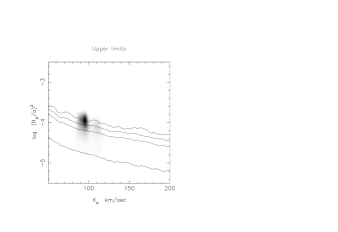
Figure 9: Relative probability map of model parameters $K_{p}$ and $\log(R_{p}/a)^{2}$, derived from the WHT/UES observations of $\tau$ Bootis, assuming the albedo spectrum to be that of a Class V roaster. The greyscale and contours are defined as in Fig. 4.

Figure 10: As for Fig. 6 but assuming a Class V spectrum for the original data without a simulated planet signal.The lower panel shows the associated reduction in $\Delta\chi^{2}$ of 12.06, measured relative to the fit obtained in the absence of any planet signal.

The “Class V roaster” is the most highly reflective of the models published by sudarsky2000. It is characteristic of planets with $T_{eff}\geq 1500$ K and/or surface gravities lower than $\sim 10$ m s^-2, and as such is associated with lower mass planets, such as $\upsilon$ And b. The model predicts a silicate cloud deck located high enough in the atmosphere that the overlying column density of gaseous alkali metals is low, allowing a substantial fraction of incoming photons at most optical wavelengths to be scattered back into space. There remains, however, a substantial absorption feature around the Na I D lines, as shown in Fig. 8.

We carried out the deconvolution using the same line list as for the grey model, but with the line strengths attenuated using the Class V albedo spectrum (see cameron02 Appendix C). We calibrated the signal strength as described in cameron02 Appendix D, by injecting an artificial planet signature consisting of the spectrum of HR 5694, attenuated by the Class V albedo spectrum and scaled to the signal strength expected for a planet with $R_{p}=1.4R_{Jup}$.

The form of the Class V probability map, as shown in Fig. 9 is similar to that encountered for the grey albedo spectrum. The resulting upper limits on the planet radius are detailed at Table 4, with the corresponding false-alarm probabilities listed in Table 5. We find the feature produces a local probability maximum near $K_{p}=95$ km s^-1, with an improvement in $\Delta\chi^{2}$ over the grey albedo model of 12.06, as plotted in Fig. 10. This improvement translates to a reduced FAP (unweighted) of 3.2%, however, the position of the best-fitting $K_{p}$ matches the prior probability maximum of $K_{p}=94$ km s^-1 so closely that the overall FAP is 0.3%, substantially lower than that obtained for the grey albedo case. This suggests strongly that the features in the data that give rise to this signal originate predominantly at blue wavelengths. If the candidate feature we observe were genuine, it would indicate a Class V planet of radius $1.08(\pm 0.19)~{}R_{J}$, which is in line with with current theory [Guillot et al.1996, Burrows et al.2000].

8.2.3 Isolated Class IV model

Figure 11: Relative probability map of model parameters $K_{p}$ and $\log(R_{p}/a)^{2}$, derived from the WHT/UES observations of $\tau$ Bootis, assuming the albedo spectrum to be that of an “isolated” Class IV gas giant. The candidate feature, if genuine, corresponds to the detection of a $1.18(\pm 0.20)~{}R_{J}$ planet. The greyscale and contours are defined as in Fig. 4.

Figure 12: As for Fig. 6 but assuming a Class IV “isolated” spectrum for the original data without a simulated planet signal. The lower panel shows the associated reduction in $\Delta\chi^{2}$ of 9.227, measured relative to the fit obtained in the absence of any planet signal.

The “Class IV” models of sudarsky2000 have a more deeply-buried cloud deck than the Class V models and are probably more closely applicable to $\tau$ Boo b given its relatively high surface gravity. The resonance lines of Na I and K I are strongly saturated, with broad damping wings due to collisions with H₂ extending over much of the optical spectrum (Fig. 8).

We used the procedures described above to deconvolve and back-project the data assuming an “isolated” Class IV spectrum. Although this model does not take full account of the effects of irradiation of the atmospheric temperature-pressure structure, it is a useful compromise between the Class V models and the very low albedos found with irradiated Class IV models. The resulting time-series of deconvolved spectra is noisier than the Class V and grey-albedo versions, because lines redward of 500 nm contribute little to the deconvolution.

The probability map (Fig.11) derived from the bootstrap matched-filter analysis again shows a marginally significant candidate reflected-light feature, but for this albedo model the peak of the distribution is shifted to $K_{p}=90$ km s^-1. The fit to the data is slightly better than in the grey albedo case, giving an improvement of $\Delta\chi^{2}=9.227$ over the no-planet hypothesis. The bootstrap analysis returns an unweighted false-alarm probability of 9.2%, but the displacement of the most probable value of $K_{p}$ (90 km s^-1) away from the prior probability maximum at $K_{p}=94$ km s^-1 means the overall Bayesian FAP is 3.2%, slightly lower than in the grey albedo case.

The increase in noise associated with the extraction of the Class IV simulation produces more loosely constrained upper limits on the planetary radius, as set out in Table 4. We note that if the candidate feature were genuine, it would indicate a Class IV planet of radius $1.18(\pm 0.20)~{}R_{J}$, still in line with current expectations [Guillot et al.1996, Burrows et al.2000].

9 Conclusion

We have re-analysed the WHT echelle spectra obtained for the F7V star $\tau$ Bootis during 1998, 1999 and 2000. By assuming that

(a) the rotation of $\tau$ Bootis is tidally locked to the orbit of the planetary companion, suggesting a orbital inclination of $i\sim 40^{\circ}$, and

(b) the planet radius $R_{p}\simeq 1.2M_{Jup}$, in accordance with the general theoretical predictions of guillot96,burrows2000 and with observations of the planetary transits across HD 209458 [Charbonneau et al.2000],

we are able to rule out a reflective planet with a grey albedo greater than $p=0.39$ to the 99.9% confidence level. The alternative approach of adopting the specific grey ($p=0.3$), Class V and Class IV albedo models of sudarsky2000 places model-dependent upper limits on the planetary radius. The results indicate with 99.9% confidence that the upper limits are $1.37~{}R_{Jup}$, $1.08~{}R_{Jup}$ and $1.22~{}R_{Jup}$ respectively for the three albedo models considered.

Our analysis reveals a candidate signal of marginal significance with a projected orbital velocity amplitude of $K_{p}~{}=~{}97$ km s^-1, assuming a grey albedo spectrum. If genuine, this would suggest an orbital inclination close to $\sim 37^{\circ}$, a planet mass $M_{p}=7.28~{}(\pm 0.83)~{}M_{Jup}$ and a grey geometric albedo of $p=0.32~{}(\pm 0.13)$, assuming $R_{p}=1.2~{}R_{Jup}$. If we feign complete ignorance of the value of $K_{p}$, our bootstrap Monte Carlo simulations give a probability ranging from 3 to 15% that the detected feature is a consequence of spurious noise from the analysis. When taking into account our prior knowledge of the system these false alarm probabilities drop to below 3%.

In particular, the Class V albedo model – in which only the spectrum shortward of 550 nm is unaffected by Na I D absorption – gives a false-alarm probability of only 0.3% when the prior probability distribution for $K_{p}$ is taken into account using Bayes’ Theorem. However, we consider this is still too large an uncertainty for us to claim a bona fide detection. Our simulations show that a statistically unassailable detection should produce a clearly visible, dark streak along the planet’s trajectory in the trailed spectrogram, and no such streak is apparent even for the Class V model.

The observations in the 2000 season were conducted at orbital phases optimised to produce the strongest possible signal at a star-planet separation in velocity space sufficient to avoid blending problems. By adopting similar observing strategies on 8m-class telescopes, future reflected light searches of $\tau$ Bootis should be able to double the effective planetary signal contained in the WHT data described here, in only a small fraction of the 17 nights devoted to this search. Indeed, 2 optimally-phased clear nights on the KeckI/HIRES combination should be able to reproduce our results, whilst the increased efficiency of the HDS spectrograph would allow Subaru to achieve very close to this depth of search over the same timescale. With this in mind, we believe that $\tau$ Bootis remains a suitable target for future reflected light searches on 8m-class telescopes.

Appendix A Calibrating the Matched-filter analysis

The purpose of incorporating a simulated planet signature into our analysis is two-fold. First, it allows us to ensure that any planetary signal, real or simulated, is maintained through the template subtraction and deconvolution procedures and can be recovered during the subsequent matched filter analysis. In doing so we can measure the degree to which any simulated signal is attenuated and infer that any real planetary signal would suffer a similar fate. Second, by using a suitable calibration factor, we can ensure that the matched filter detection for the simulated planet, appears at the expected position in the resulting $\log(\epsilon_{0})=\log~{}p(R_{p}/a)^{2}$ vs $K_{p}$ probability map, i.e. at $\log(\epsilon_{0})=-4.01$ in Fig. 4. Thus any potential detections within the real data (Fig. 5) would be suitably compensated for losses imposed by the extraction and analysis procedures.

We model the reflected-light signal as a time sequence of Gaussians with appropriate velocities and relative amplitudes according to

$$G(v,\phi,K_{p}) = \frac{W_{*}}{\Delta v_{p}\sqrt{\pi}}g(\phi,i)\times$$ (9)

$$\times\exp\left[-\frac{1}{2}\left(\frac{v-K_{p}\sin\phi}{\Delta v_{p}}\right)^{2}\right].$$

where the amplitude $K_{p}$ of the sinusoidal velocity variation is determined by the system inclination and stellar mass.

The variable factor we use to calibrate the strength of the detected signal is the equivalent width ($W_{*}$) of the stellar component of the composite line profile. By deconvolving the observed spectrum of HR 5694 with a list of the relative strengths of its spectral lines, we obtain a composite line profile exhibiting the broadening function that is representative of all the lines recorded in the spectrum. The deconvolved line profile is shown at Fig. 13 alongside that for $\tau$ Bootis itself. We recall that HR 5694 was chosen to best mimic the non rotationally broadened line profiles reflected from the near tidally locked planet.

Figure 13: Deconvolved line profiles for HR 5694 and $\tau$ Bootis, showing the average broadening exhibited by all lines within their echelle spectra. The line profiles exhibit significantly different shapes due to the difference between the two stars’ rotation rates. The normalised equivalent widths of the line profiles are $W_{*}$ = 4.45 and $W_{*}$ = 4.42 respectively.

The planet signal should take the form of a faint copy of the stellar spectrum, as sharp as the deconvolved profile of HR 5694, located deep within the noise of the composite deconvolved residual profile of $\tau$ Bootis, i.e. the deconvolved profile of the residual $\tau$ Bootis spectrum following stellar subtraction.

In effect the matched-filter analysis compares the $W_{*}$ value with the strength of the best fit Gaussian filter from the phased residual profiles, as at Fig. 2. Ideally, by using $W_{*}$ = 4.45, any simulated planet signal should be recovered at the correct level within the $\log(\epsilon_{0})$ vs $K_{p}$ probability map. However, analysis of the dataset following injection of a synthetic planet signal showed a 15% reduction in the equivalent width ($W_{*}$ = 3.85) was required to recover the fake grey albedo planet’s signal at the correct strength. Any reduction in the strength of the simulated signal during the various processes would indeed manifest itself as a reduction in the $\log(\epsilon_{0})$ scaling factor, and would thus appear fainter than expected, necessitating a correction to $W_{*}$. It is found that each of the extraction processes contributes to the signal reduction, with the PCA fixed noise removal (cameron02 Appendix B) contributing 9% to the total loss. Any genuine reflected light signal should undergo a similar loss. In calibrating the grey albedo model (Section 8.2.1) we have therefore needed to correct for this signal loss during the extraction process. Similar, but less significant corrections ($\sim$ 10%) had to be applied to the Class IV and Class V models in order to calibrate the $(R_{p}/a)^{2}$ values produced by the matched-filter analysis.

References

- [\citefmtBaliunas et al.1997] Baliunas S., Henry G., Donahue R., Fekel F., Soon W., 1997, ApJ, 474, 119
- [\citefmtBrown et al.2001] Brown T., Charbonneau D., Gilliland R., Noyes R., Burrows A., 2001, ApJ, 552, 699
- [\citefmtBurrows et al.2000] Burrows A., Guillot T., Hubbard W., M. M., Saumon D., Lunine J., Sudarsky D., 2000, ApJ, 534, 97
- [\citefmtButler et al.1997] Butler P., Marcy G., Williams E., Hauser H., Shirts P., 1997, ApJ, 474, 115
- [\citefmtCameron et al.1999] Cameron A., Horne K., Penny A., James D., 1999, Nat, 402, 751
- [\citefmtCameron et al.2002] Cameron A., Horne K., Penny A., Leigh C., 2002, Monthly Notices of the Royal Astronomical Society, 330, 187
- [\citefmtCharbonneau et al.1999] Charbonneau C., Noyes D., Jha S., Vogt S., 1999, ApJ, 522, 145
- [\citefmtCharbonneau et al.2000] Charbonneau D., Brown T., Latham D., Mayor M., 2000, ApJ, 529, 45
- [\citefmtCharbonneau et al.2002] Charbonneau D., Brown T., Noyes R., Gilliland R., 2002, ApJ, 568, 377
- [\citefmtCollier Cameron et al.2001] Collier Cameron A., Horne K., James D. J., Penny A. J., Semel M., 2001, in Penny A., Artymowicz P., Lagrange A.-M., Russell S., eds, IAU Symp. 202: Planetary systems in the Universe. ASP Conference Series, San Francisco, In press: astro-ph0012186
- [\citefmtDonati et al.1997] Donati J. F., Semel M., Carter B., Rees D. E., Collier Cameron A., 1997, Monthly Notices of the Royal Astronomical Society, 291, 658
- [\citefmtFuhrmann, Pfeiffer & Bernkopf1998] Fuhrmann K., Pfeiffer J., Bernkopf J., 1998, Astronomy and Astrophysics, 336, 942
- [\citefmtGonzalez1998] Gonzalez G., 1998, Astronomy and Astrophysics, 334, 221
- [\citefmtGuillot et al.1996] Guillot T., Burrows A., Hubbard W., Lunine J., Saumon D., 1996, ApJ, 459, 35
- [\citefmtHenry et al.2000] Henry G., Baliunas S., Donahue R., Fekel F., Soon W., 2000, ApJ, 531, 415
- [\citefmtHilton1992] Hilton J., 1992, Expanatory supplement to Astronomical Almanac. University Science Books, Mill Valley, CA
- [\citefmtHovenier1989] Hovenier J., 1989, Astronomy and Astrophysics, 214, 391
- [\citefmtHubbard et al.2001] Hubbard W., Fortney J., Lunine J., Burrows A., Sudarsky D., Pinto P., 2001, ApJ, 560, 413
- [\citefmtMarley, Gelino & Stephens1999] Marley M., Gelino C., Stephens D., 1999, ApJ, 513, 879
- [\citefmtMayor & Queloz1995] Mayor M., Queloz D., 1995, Nat, 378, 355
- [\citefmtPerryman, Lindegren & Kovalevsky1997] Perryman M., Lindegren L., Kovalevsky J., 1997, Astronomy and Astrophysics, 323, 49
- [\citefmtSeager & Sasselov1998] Seager S., Sasselov D., 1998, ApJ, 502, 157
- [\citefmtSeager, Whitney & Sasselov2000] Seager S., Whitney A., Sasselov D., 2000, ApJ, 540, 504
- [\citefmtSudarsky, Burrows & Pinto2000] Sudarsky D., Burrows A., Pinto P., 2000, ApJ, 538, 885
Acknowledgements
This work is based on observations made with the William Herschel Telescope, operated on the island of La Palma by the Isaac Newton Group in the Spanish Observatorio del Roque de los Muchachos of the Instituto de Astrofisica de Canarias. The initial data reduction was carried out using the ECHOMOP and FIGARO software supported by the Starlink Project, on PC/Linux hardware funded through a PPARC rolling grant. ACC and KDH acknowledge the support of PPARC Senior Fellowships during the course of this work.
We thank David Sudarsky and Adam Burrows for providing us with listings of their Class IV and Class V albedo models. We also thank Geoff Marcy for his updates on the orbital ephemeris of Boo b.