An Intrinsic Absorption Complex Toward RX J$1230.8+0115$: Geometry and Photoionization Conditions

Abstract

We present HST/STIS and FUSE spectra of the quasar RX J$1230.8+0115$ ($V=14.4,z=0.117$). In addition to Galactic, Virgo, and intervening absorption, this quasar is host to a remarkable intrinsic absorption complex. Four narrow absorption line systems, strong in C iv, N v, and O vi, lie within $5000$ km s^-1 of the QSO redshift. Three of the systems appear to be line-locked, two in N v, and two in O vi, with the common system residing in between the other two (in velocity). All three systems show signs of an intrinsic origin – smooth wind-like profiles, high ionization, and partial coverage of the central engine. The fourth system, which appears at the systemic redshift of the QSO, may originate from host galaxy or intervening gas. Photoionization analyses imply column densities in the range $19.1<\log N$(H) $<21$ and ionization parameters in the range $-1.3<\log U<0.3$. Revisiting the issue of line-locking, we discuss a possible model in the context of the accretion-disk/wind scenario and point out several issues that remain for future simulations and observations.

1. Introduction

Narrow absorption lines due to gas that is truly intrinsic to the central engines of quasi-stellar objects (QSOs) have recently been recognized as ubiquitous (Richards et al., 1999). They are a powerful diagnostic of the physical conditions of the gas (e.g., Hamann et al., 1997a; Crenshaw et al., 1998; Hamann et al., 2000; Kraemer et al., 2001) since they arise from a wide range of ionization conditions. Still, the origins of this gas and its relationship to other regions (e.g., the broad emission line region; hereafter, the BLR) is uncertain. There are indications that many of the associated absorption lines (narrow absorption lines that arise within $5,000$ km s^-1 of the QSO emission redshift) are indeed connected to the BLR (Ganguly et al., 2001a), and to the X-ray “warm” absorbers (e.g., Mathur et al., 1995; Brandt et al., 2000). Strong [$W_{\mathrm{r}}\gtrsim 1.5$ Å] associated absorbers seem to appear preferentially in optically-faint, steep-spectrum, radio-loud objects (Møller & Jakobsen, 1987; Foltz et al., 1988; Aldcroft et al., 1994), while “high ejection velocity” absorbers tend to appear in the spectra of radio-quiet and flat-spectrum objects (Richards et al., 1999).

Another puzzle regarding intrinsic narrow absorption is the origin of complexes of intrinsic lines. Here, a complex of absorption lines means a group of narrow absorption line systems, which are well separated in velocity, along a particular line of sight where the local redshift path density is much larger than expected from randomly distributed intergalactic gas. This is observationally distinct from the substructure that nearly all absorption line systems (intrinsic or intervening) exhibit at high spectral resolution. There are many examples of intrinsic absorption systems (with single profiles) which show substructure (e.g., Korista et al., 1993; Crenshaw et al., 1999; Ganguly et al., 1999). While several examples of absorption lines complexes now exist in the literature (e.g., Foltz et al., 1987; De Kool et al., 2001; Ganguly et al., 2001b; Richards et al., 2002a; Misawa et al., 2003), their origin has not yet been fully explored. Some fraction of complexes may represent cosmological “superstructure,” but others result from gas intrinsic to the background quasar. While a small fraction of sightlines are expected to contain excesses of absorption line systems, the incidence of absorption line complexes has not yet been sufficiently constrained to infer the relative contributions of these two scenarios. In the cases where such complexes are due to intrinsic gas, they represent an important constraint on unification models designed to explain intrinsic absorption. Under the intrinsic hypothesis, it is unclear how line complexes relate to broad absorption lines, to single intrinsic narrow absorption lines with extensive substructure, or even to the properties of the “host” QSO. In this paper, we report an intrinsic absorption line complex toward the QSO RX J$1230.8+0115$ ($V=14.42$, $z_{\mathrm{em}}=0.117$, $\nu L_{\nu}$(2500 Å)$=2.8\times 10^{44}~{}\mathrm{erg~{}s}^{-1}$).

RX J$1230.8+0115$ was first detected by the ROSAT All-Sky Survey (Read, Miller, & Hasinger, 1998). It is located $54^{\prime}$ from 3C 273 on the sky and is one of the brightest QSOs in the optical band. It hosts a complex of four absorption lines (detected in H i, C iv, N v, and O vi) in the ejection velocity range $-4600<v_{\mathrm{ej}}<-215$ km s^-1, three of which are likely to have an intrinsic origin. In §2, we present high resolution Hubble Space Telescope (HST) and intermediate resolution Far Ultraviolet Spectroscopic Explorer (FUSE) spectra of RX J$1230.8+0115$, and a description of the complex. In §3, we show that the complex has an intrinsic origin. In §4, we characterize the photoionizing spectrum and present results from Cloudy (Ferland, 2001) simulations to constrain the physical conditions of the gas. We summarize our results in §5. Finally, in §6, we discuss the implications of our results in the broader picture of intrinsic absorbers and intrinsic absorption complexes and point out avenues (both theoretical and observational) for further research.

2. Data

RX J$1230.8+0115$ has been observed several times by HST for the purpose of examining Ly $\alpha$ absorption in the local universe (Impey, Petry, & Flint, 1999; Penton, Shull, & Stocke, 2000a, b). More recently, RX J$1230.8+0115$ was observed for 27.2 ksec in January 1999 with the Space Telescope Imaging Spectrograph (STIS) using the E140M echelle, $0.\!^{\prime\prime}2\times 0.\!^{\prime\prime}06$ slit, and the FUV-MAMA detector (under proposal 7737 by Michael Rauch). The resolving power of this configuration is $R\sim 45,600$ (6.6 km s^-1 velocity resolution) with two pixels per resolution element. The reduction of the raw data and calibration of the reduced data followed the standard HST/STIS pipeline software (the CALSTIS package in IRAF). According to the CALSTIS documentation (Brown et al., 2002), the absolute wavelength calibration is good to within a pixel (0.015 Å at 1425 Å, the central wavelength), and the absolute photometry is good to 8% ($\sim 2\times 10^{-15}~{}\mathrm{erg~{}cm}^{-2}~{}\mathrm{s}^{-1}~{}\mathrm{\AA}^{-1}$). The fully reduced and calibrated spectrum, covering the wavelength range 1178.2–1723.8 Å, is presented in Fig. 1. The data have been resampled to combine overlapping regions of the echelle orders. In the figure, the spectra have also been rebinned ($2\rightarrow 1$) to resolution element, not pixel, samples. Superimposed on the data is the effective continuum (continuum $+$ emission lines) fit. The lower trace in each panel is the error spectrum.

RX J$1230+0115$ was observed by FUSE on 20 Jun 2000 for a total exposure time of 4 ksec. The four FUSE channels were co-aligned during the observation, and signal was detected across the full FUSE bandpass (905-1187 A). We retrieved the raw data from the FUSE archive (observation set P1019001) and calibrated the data for each detector segment using the latest version of CALFUSE (v2.1.6). CALFUSE screens the photon event lists for valid data, performs geometrical distortion corrections, and calibrates the one dimensional spectra extracted from the two dimensional spectral images. After spectral extraction, we checked the heliocentric wavelength calibration of each segment by comparing common spectral regions recorded in different data segments.

For this analysis, we restrict our attention to data from the LiF1b and LiF2a channels which cover the wavelength range 1086.4–1184.8 (shown in Fig. 2) since the data from the SiC1 and SiC2 channels have low $S/N$. We binned the data into 5-pixel bins to improve $S/N$, while maintaining the full velocity resolution of the data. (The raw data are oversampled at 10–12 pixels per resolution element.) We estimate $S/N=4(5)$ per 20 km s^-1 resolution element at 1150 Å for the LiF1b (LiF2a) channel.

We note here that, while RX J$1230.8+0115$ is an X-ray selected quasar, there are no X-ray observations that are of sufficient quality to extract a spectrum. A search in the heasarc archive reveals only one “direct” observation - that of the ROSAT All-Sky Survey. While there are several pointed observations of 3C 273, RX J$1230.8+0115$ is at the edge of these fields where the point-spread function is large, and the there are insufficient counts to create a spectrum. An observation with Chandra or XMM-Newton would be very revealing in regards to a possible “warm absorber” phase.

2.1. Line Identifications and Measurements

Our method for detecting absorption features followed the prescription from Lanzetta, Wolfe, & Turnshek (1987). This method creates a smoothed equivalent width spectrum from both the normalized flux and the normalized errors (the sigma). A pixel records absorbed flux if the smoothed equivalent width ($W_{\mathrm{i}}$) exceeds the error ($\sigma_{\mathrm{i}}$) by a user-defined threshold (i.e., $W_{\mathrm{i}}/\sigma_{\mathrm{i}}>n$). In this case, we set our detection limit to $1.5\sigma$.

At this low confidence level, our completeness limit for detecting real features of a given equivalent width is improved, but the number of false detections is increased. We are 95% complete down to a limiting equivalent width of $0.10$ Å at $1.5\sigma$ confidence. This limit increases to $0.31$ Å at $4.5\sigma$ confidence. To limit the false detection of an absorption system, we require the detection of multiple species – a spectral doublet (N v $\lambda\lambda 1238.8,1242.8$ or C iv $\lambda\lambda 1548.2,1550.7$) and Ly $\alpha$. To characterize the false detection rate of this approach, we simulated 1000 noise realizations using the error spectrum from the STIS-E140M observation and looked for sets of features that (falsely) satisfied the N v $\lambda\lambda 1238.8,1242.8$$+$Ly $\alpha$ detection criterion. In these realizations, 3517 features were detected at $1.5\sigma$ confidence that could potentially yield an absorption system in the redshift range $0<z<0.1358$ in N v $\lambda\lambda 1238.8,1242.8$ and Ly $\alpha$. (The upper redshift limit arises from the canonical upper limit for associated systems: 5000 km s^-1 beyond the quasar emission redshift.) Since our criterion for the selection of a system requires the detection of a set of three lines, 3517 features translates to $7\times 10^{9}$ potential systems - the number of ways of choosing a set of 3 lines from a sample of 3517. Of the $7\times 10^{9}$ sets of features, $5\times 10^{5}$ satisfied the N v doublet$+$Ly $\alpha$ spacings and therefore would have been identified (falsely) as an absorption system. This implies a false detection rate of $5\times 10^{5}/7\times 10^{9}=7\times 10^{-5}$. Thus, in spite of the low ($1.5\sigma$) confidence for “detecting” features, our confidence threshold for identifying a system is 99.993% (effectively $4\sigma$).

To identify other features with absorption systems, we compiled a list of resonant transitions covered by the spectrum for any possible absorber between the Galaxy and the QSO. With both the STIS-E140M spectrum and FUSE LiF spectra, the effective observed wavelength range is 1128.3–1723.8 Å. (Due to the redshift of the quasar, we include in our line-list transitions down to a rest-frame wavelength of 1010.1 Å.) After identifying Galactic lines, we culled the list of detected features using the aforementioned criteria with the N v $\lambda\lambda 1238.8,1242.8$ and C iv $\lambda\lambda 1548.2,1550.7$ doublets. As a further constraint, the resulting candidate systems were checked by hand to ensure that doublets had similar kinematic structures. In the end, we identified six metal-line systems, four of which lie within $5000$ km s^-1 of the QSO emission redshift. These four systems are described in the next section. [One of the other two systems is absorption by the Virgo Southern Extension. This system has been examined by Ganguly, Sembach, & Charlton (2003) and Rosenberg et al. (2003).] In Fig. 3, we show the detected transitions of the complex from H i, C iv, N v, and O vi aligned in velocity with the zero-point at $z_{\mathrm{em}}=0.117$.

2.2. Associated Absorption Systems

• 0.1000: (System A in Fig. 3) This is a weak system that is detected in H i, C iv, N v, and O vi. The O vi $\lambda\lambda 1031.9,1037.6$ transitions in this system are apparently line-locked with the Ly $\beta$ and O vi $\lambda 1031.9$ transitions from System B at $z_{\mathrm{abs}}=0.1058$. The O vi $\lambda 1031.9$ line is blended with Galactic absorption by the N i$\lambda\lambda\lambda 1134.2,1134.4,1135$ triplet.

• 0.1058: (System B in Fig. 3) This system is detected in H i, C iv, N v, and O vi. This system is apparently line-locked in the N v $\lambda\lambda 1238.8,1242.8$ doublet with that from the $z=0.1093$ system (System C). The system is also apparently locked with the $z=0.1000$ system (System A) in the O vi $\lambda\lambda 1031.9,1037.6$ doublet (as mentioned above). The C iv doublet for this system is self-blended (with a width larger than the doublet separation) so this is not a classic narrow absorption line system. The smooth troughs of all the transitions are characteristic of wind kinematics. In addition, the N v$\lambda 1232.8$, and H i Ly $\beta$ lines are blended with the Ni ii$\lambda 1370.1$ and N i$\lambda\lambda\lambda 1134.2,1134.4,1135$ Galactic absorption, respectively. This type of system has been referred to as a mini-BAL (e.g., Turnshek, 1988; Barlow, Hamann, & Sargent, 1997; Churchill et al., 1999), a relatively narrow version of a BAL.

• 0.1093: (System C in Fig. 3) This system is detected in H i, C iv, N v, and O vi. The N v$\lambda 1238.8$ transition for this system is blended with the N v$\lambda 1242.8$ transition of System B (as mentioned above) and the O vi $\lambda 1031.9$ line is blended with Galactic Fe ii $\lambda 1144.9$ absorption. The profiles of this system are also smooth, indicative of an outflowing-wind origin. For clarification, we note that the line at 1374.2 Å, misidentified by Impey et al. (1999) as a Ly $\alpha$ absorber at $z_{\mathrm{abs}}=0.1301$ from a low resolution HST/GHRS-G140L spectrum, is actually the blend between N v$\lambda 1242.8$ at $z_{\mathrm{abs}}=0.1058$ and N v$\lambda 1238.8$ at $z_{\mathrm{abs}}=0.1093$. The blending of the N v doublet is clear from the higher resolution spectrum presented here.

• 0.1162: (System D in Fig. 3) This system is detected in H i, N v, and O vi. The O vi $\lambda 1031.9$ line is blended with Galactic P ii $\lambda 1152.8$. The redshift actually places this system redward of the N v emission line peak, although the velocity matches the QSO systemic redshift (as measured using Balmer lines). The kinematic structure of this system clearly motivates the idea that the absorption arises from a clumpy medium (at least along the line of sight). Another clarifying note: The N v$\lambda 1242$ feature for this system was misidentified by Impey et al. (1999) as a Ly $\alpha$ absorber at $z_{\mathrm{abs}}=0.1419$.

3. Are They Truly Intrinsic?

3.1. Circumstantial Evidence

We examine three avenues of circumstantial evidence that point toward an intrinsic origin of the absorbing gas in this complex. In order of increasing reliability, we discuss the probability of detecting these systems in the redshift path, the probability for chance superposition of lines (“line locking”), and the high ionization state of the absorbers.

3.1.1 Redshift Path Density of Absorbers

The first clue that these absorbers have an intrinsic origin comes from the low probability that they arise from uncorrelated gas (i.e., intergalactic clouds), as expected if the absorbers were cosmologically distributed. In this sightline, six metal-line systems are detected in the C iv $\lambda\lambda 1548.2,1550.7$ doublet and four in the N v $\lambda\lambda 1238.8,1242.8$ doublet down to a limiting equivalent of $W>10$ mÅ over a redshift path of $\delta z=0.1162$. According to the HST Quasar Absorption Line Key Project, on average we expect to detect 0.11 C iv absorbers and 0.01 N v absorbers in this redshift path down to a 95% completeness limit of 1 Å. At this same equivalent width limit, we detect only 1 C iv system and 2 N v systems. The Poisson probability of finding 1 C iv system (2 N v systems) when only 0.11 (0.01) are expected is 0.10 ($5\times 10^{-5}$). Based on the statistics of N v absorbers, it is probable that the absorbers are correlated. In the next section, we examine the likelihood of observing three apparently line-locked metal-line systems if the systems are uncorrelated.

3.1.2 Apparent Line-Locking of Systems

We performed a Monte Carlo simulation to determine the chance probability of detecting apparent line-locking among four N v systems placed randomly over a redshift path. Two systems are taken to be apparently line-locked if the velocity separation matches that of the N v $\lambda\lambda 1238.8,1242.8$ doublet, 964.5 km s^-1, to 90% confidence. (In the simulations, we used the velocity widths of the four associated systems: 40, 137, 65, 63 km s^-1.) For a redshift path of $\Delta z=0.0333$ (corresponding to the velocity window for “associated” systems), the probability of a chance superposition between two systems is 0.070. (The probability is similar for the O vi doublet separation.) The binomial probability of finding two apparently line-locked pairs, from a sample of 6 pairs (4 absorption systems yields 6 pairs) is 0.055. Thus, it is unlikely that the apparent line-locking of systems in this sightline is due to random chance.

3.1.3 High Ionization State

High ionization structure is used (usually in tandem with other evidence) as a sign of an intrinsic origin for absorbers, since the gas is subject to photoionization by the quasar continuum (e.g., Hamann et al., 1995; Barlow & Sargent, 1997). It is readily seen (before detailed photoionization modelling) that the absorbers are highly ionized. There is no Lyman limit detected in the FUSE spectrum, so all the H i column densities must be $<10^{17.2}~{}\mathrm{cm}^{-2}$ assuming no dilution by unocculted flux. The N v and C iv absorption profiles are very strong compared to their Ly $\alpha$ profiles; in fact, N v appears to be saturated in the case of system B. Finally, while the Si iii$\lambda 1206.5$ and Si iv $\lambda\lambda 1393.8,1402.8$ lines are covered by the STIS-E140M spectrum, they are not detected down to limiting (3$\sigma$) equivalent widths of $\sim 0.01$ Å (for Si iii) and $\sim 0.03$ Å (for Si iv). These limits correspond to column density limits of $N$(Si iii)$\lesssim 10^{11.7}~{}\mathrm{cm}^{-2}$ and $N$(Si iv)$\lesssim 10^{12.5}~{}\mathrm{cm}^{-2}$ assuming there is no dilution by unocculted flux.

3.2. Direct Evidence

Since the spectral resolution of the STIS-E140M observation is good enough (FWHM$\approx$6–7 km s^-1) to fully resolve the kinematics of the profiles, it is possible to apply a test to determine if the associated absorbers are truly intrinsic. Using the well-separated N v $\lambda\lambda 1238.8,1242.8$ and C iv $\lambda\lambda 1548.2,1550.7$ doublets, one can infer the fraction of the background flux incident on the absorber. Normally this is done by using the flux in corresponding pixels of the two doublet profiles. This can be done as a function of velocity (e.g., Arav et al., 2002) by computing the coverage fraction across the entire profile, or as a function of kinematic component (e.g., Hamann et al., 1997a) by using the flux in the cores of the components. The premise behind this approach is that profiles are diluted by flux that is not incident on the absorber. The apparent attenuation of the lines is given by:

$$I(v)=1-C(v)+C(v)e^{-\tau(v)}.$$ (1)

Invoking the atomic physics constraint that the true optical depths of the spectral doublet transitions have a 2:1 ratio yields the standard solution for the coverage fraction as a function of velocity:

$$C(v)={{(I_{\mathrm{w}}(v)-1)^{2}}\over{I_{\mathrm{s}}(v)-2I_{\mathrm{w}}(v)+1}},$$ (2)

where $I_{\mathrm{s}}$ and $I_{\mathrm{w}}$ are the normalized flux profiles of the stronger and weaker transitions, respectively. Due to instrumental effects, a pixel-by-pixel computation (i.e, computations across the entire profile) is not trustworthy in the wings of profiles even if the profiles are well resolved (Ganguly et al., 1999). In passing, we also note that the correct geometric interpretation of the coverage fraction is not clear. (For example, light scattered around the absorbing gas can produce coverage fractions less than unity.)

In the case of this complex, it is only possible to apply a pixel-by-pixel approach to three doublets – the N v $\lambda\lambda 1238.8,1242.8$ doublet for systems A and D, and the C iv $\lambda\lambda 1548.2,1550.7$ doublet for system C. No doublets for system B are sufficiently “clean” for this approach, and the FUSE spectra are not off sufficient quality to apply this to the O vi $\lambda\lambda 1031.9,1037.6$ profiles. In Fig. 4, we show two panels for each system that test for the existence of partial coverage in these doublet profiles. The top panels show the apparent column densities (Savage & Sembach, 1991, hereafter, ACD) of the doublet transitions (and differences therein). When profiles are resolved and apparently unsaturated, the ACD profiles from both transitions should coincide. The signature of partial coverage is that the weaker transition will imply a larger ACD than the stronger transition, although this can also result from unresolved saturation. In the bottom panels, we show the normalized flux profile from the stronger transition and the pixel-by-pixel coverage fraction (from eq. 2). Coverage fractions are plotted as per the criteria of Ganguly et al. (1999).

The N v doublet for system A clearly shows evidence for partial coverage from both the ACD and pixel-by-pixel coverage fraction profiles. The C iv doublet toward system C shows no evidence for partial coverage. System D shows marginal evidence at the core of the strongest component from the ACD plot, but not in the coverage fraction plot. This may be unresolved saturation from a narrow component.

In the interest of extracting column densities for all absorption components, we employed a profile fitting technique that separately accounts for the partial coverage fractions and column densities. We model the profiles as arising from discrete, Gaussian-broadened components which only partly occult the backround source. In the limit where this is applicable, each component givesrise to an effective attenuation factor given by Eq. 1 and the observed profile is given by the product of these factors.

$$I(\lambda)=I_{\mathrm{o}}(\lambda)\prod_{i=1}^{n}\prod_{j=1}^{m(i)}\left[1-C_{\mathrm{i}}+C_{\mathrm{i}}e^{-\tau_{\lambda}(z_{\mathrm{i}};N_{\mathrm{ij}},b_{\mathrm{ij}})}\right],$$ (3)

where $n$ is the number of absorption components, $m(i)$ is the number of ionic species associated with component $i$, $C_{\mathrm{i}}$, and $z_{\mathrm{i}}$ are the partial coverage fraction and redshift of the $i^{\mathrm{th}}$ component, and $N_{\mathrm{i}}$, and $b_{\mathrm{ij}}$ are the column density, and velocity width of the $j^{\mathrm{th}}$ species of component $i$. In the case where the entire flux from the quasar is incident on all the absorbers (e.g., an intervening absorber), this reduces to the exponential of the sum of optical depths, $I(\lambda)=I_{\mathrm{o}}(\lambda)\exp[-\sum\tau(\lambda)]$. In the case where the absorbers are optically thick at the observed wavelength, this reduces to the product of non-incident fractions, $I(\lambda)=I_{\mathrm{o}}(\lambda)=\prod(1-C_{\mathrm{i}})$.

In the application to this complex, we first fit the absorption “by-hand”, using the minimum number of components possible and the number of troughs in each system as an indication of the number of components – one component for system A, four for system B, three for C, and five for D. The result was run through the Numerical Recipes Levenberg-Marquardt $\chi^{2}$-minimizing routines mrqmin and mrqcof (Press et al., 1992) for optimization and error analysis. The optimization procedure minimizes the $\chi^{2}$ statistic and only retains components that significantly reduce $\chi^{2}$ to 80% confidence (this is assessed using the F-test for $\chi^{2}$ significance). We constrain the coverage fraction and column density separately for each detected ion. Coverage fractions are allowed to vary on the (physically meaningful) range [0,1]. Column densities are allowed to vary such that the optical depth in the strongest transition lies in the range [0,3]. Beyond this range, the component is deemed “saturated” and only a lower limit on the column density is reported. We tie the redshift and velocity width of each the absorption component across all detected ions and assume Gaussian line-broadening. In other words, the redshift and velocity width were allowed to vary, but not separately from ion to ion. (As a first step, we separately constrained the contributions of thermal and non-thermal broadening to the line widths; the thermal contribution was found to be negligible.) We accounted for the Galactic Ni ii$\lambda 1370$ absorption, which blends with the N v$\lambda 1238$ absorption in System B, by simultaneously fitting the Ni ii$\lambda 1317$ line which has similar strength. The optimization procedure threw out one component from system B (since the absorption could be explained through the Galactic Ni ii) and one component from system C; the results appear in Table 1. We list the component name (column 1), redshift (column 2), velocity width (column 3), H i column density (column 4), C iv column density and coverage fraction (columns 5 and 6, respectively), and N v column density and coverage fraction (columns 7 and 8, respectively). The $1\sigma$ fitting uncertainties for each parameter are listed beneath each value.

We overlay the fit and the component contributions in Fig. 3. For ions where only a single transition is detected, the measurement of the coverage fraction and column density are degenerate unless the transition is saturated. In these cases, “measured” values are to be taken lightly. Since the FUSE spectrum is neither of high spectral resolution, nor of high signal-to-noise, we were unable to reasonably (and directly) constrain the column densities and coverage fractions of O vi and H i (using the higher Lyman series lines). Since the Ly $\alpha$ transition for H i is covered by the STIS echelle spectrum, we obtained a lower limit on the H i column density by fixing the coverage fraction at unity.

Systems A, B, and C appear to require partial coverage to fit the N v and C iv doublet profiles. Thus, it is likely that the absorbing gas is close to the central engine. We note that the partial coverage fractions reported for the “clean” systems (described above) are consistent with those yielded by the direct inversion. We also note that the absorption troughs are sufficiently deep to imply that both continuum and broad emission line photons are absorbed. Thus, the absorbers must either lie beyond or be co-spatial with the broad line region. System D does not require any partial coverage. Given the clumpiness of the absorption and the closeness to the systemic redshift, it is possible that this is absorption by the host galaxy. In the next section, we use the measurements of the column densities and Cloudy simulations to constrain the physical conditions of the absorbers.

4. Physical Conditions of the Intrinsic Absorption Complex

To constrain the physical conditions of the components, we applied Cloudy photoionization models to compare the C iv and N v column densities.

4.1. Characterization of the Ionizing Spectrum

In our efforts to perform detailed photionization models of the absorbers, we used the available X-ray, ultraviolet, and radio data to characterize the photoionizing spectrum from the QSO. The QSO is not detected by the FIRST survey (Becker et al., 1995) down to a limiting flux of 3.45 mJy, implying a 5 GHz luminosity density $L_{\nu}<10^{30.5}\,\mathrm{erg~{}s}^{-1}~{}\mathrm{Hz}^{-1}$. The QSO is radio-quiet and we assume an X-ray energy index $\alpha_{\mathrm{x}}=-1.69$ (Laor et al., 1997). The ROSAT All-Sky Survey detection of the QSO reports a count rate of $0.04\pm 0.01$ counts s^-1 in the 0.1–2 keV band. Using the HEASARC WebPIMMS count rate-to-flux converter, we calculate $F_{\mathrm{\nu}}(2~{}\mathrm{keV})=(3.0\pm 1.0)\times 10^{-31}~{}\mathrm{erg~{}cm}^{-2}~{}\mathrm{s}^{-1}~{}\mathrm{Hz}^{-1}$ assuming a power law model with Galactic absorption [$N(\mathrm{H})=1.83\times 10^{20}~{}\mathrm{cm}^{-2}$ (Dickey & Lockman, 1990)]. From a power-law fit to the STIS-E140M spectrum, excluding emission lines, we constrain the ultraviolet energy index to be $\alpha_{\mathrm{o}}=-1.0$, with $F_{\mathrm{\nu}}(2500~{}\mathrm{\AA})=8.4\times 10^{-27}~{}\mathrm{erg~{}cm}^{-2}~{}\mathrm{s}^{-1}~{}\mathrm{Hz}^{-1}$. From this, we infer $\alpha_{\mathrm{ox}}=-1.71$. For the ionizing spectrum, we used the Cloudy AGN spectrum with the following parameters: $T=150,000~{}{\mathrm{K}}$ (the default), $\alpha_{\mathrm{ox}}=-1.71$, $\alpha_{\mathrm{o}}=-1.0$, $\alpha_{\mathrm{x}}=-1.69$.

We ran a two-dimensional grid of Cloudy models stepping through total hydrogen column densities [$N(\mathrm{H})$] and ionization parameters ($U$). (The ionization parameter is defined as the ratio of the number density of hydrogen ionizing photons to the total hydrogen number density.) For each model, we chose a plane-parallel slab geometry with solar abundances, and a nominal hydrogen space density of $3000~{}\mathrm{cm}^{-3}$ (e.g., Hamann et al., 1997a). The ionizing continuum was normalized by the specification of the ionization parameter. For a given ionization parameter, the space density of the gas and the source-absorber distance are degenerate through the luminosity of the quasar ($U\propto L/nr^{2}$). For an ionization parameter of $U=0.1$, the effective distance is $r\sim 270$ pc. Through the degeneracy, the absorbers may be closer to the central engine if they are denser than the assumed value. Since we do not have an independent measure of the density (e.g., from detections of excited state lines or from time variability of absorption profiles), we cannot use the photoionization models to constrain either the source-absorber distance, or the absorber thickness. Through simulations, we have verified that the inferred ionization parameters and total hydrogen column density are largely independent on the choice of space density (over at least three decades). For a given $U$ and $N$(H), increasing the space density of an absorber will bring it closer to the ionizing source and also make it smaller (i.e., the thickness decreases to match the column density).

4.2. Total Column Densities and Ionization Parameters

Using the measured C iv and N v column densities (which are automatically corrected for the covering fraction by the fitter) and the H i column density limit, we constructed column density isopleths for each ion in $N(\mathrm{H})-U$ space. In principle, the intersection of these isopleths uniquely specifies both $N(\mathrm{H})$ and $U$ for each absorption component. In Fig. 5, we use these contours to generate $1\sigma$-confidence allowed regions of $N$(H)-$U$ for components A1, B1, B2, B3, and C3. In Table 2, we report the optimal values for $N$(H) and $U$ for components B1, B2, and C2, and limiting constraints for components A1 and B3. For component B2, Si iii and Si iv are overproduced by $\sim 0.2$ dex. That is, the column density limits (from §3.1) are not satisfied. There is not enough information provided by the data to examine the reason for this. Possible reasons include an artifact of Gaussian line-broadening, abundance variations, or partial coverage effects.

In the same table, we also report the predicted H i and O vi column densities based on the best-fit physical conditions. Using these predicted column densities, we constrain the H i and O vi coverage fractions of the components using the profile fitter, fixing the column densities and kinematics. These are also listed in the table. No low ionization species (e.g., C ii, Si ii) were detected in these spectra. Such detections would provide constraints on the density (in conjunction with the corresponding strong high excitation lines), which would further constrain the relation. More importantly, it would be prudent to obtain column densities of higher ionization species to constrain the ionization parameter. Using only N v and C iv column densities is problematic when the ionization parameter is $U\gtrsim 0.2$, since small uncertainties in the column densities propagate to large uncertainties in $N(\mathrm{H})$ and $U$.

5. Summary of Results

The ultraviolet spectrum of RX J$1230.8+0115$ hosts a complex of associated narrow absorption line systems detected in H i, C iv, N v, and O vi. Before detailed analysis, there are a few striking properties of this complex to note. First, the four systems reside in a $5000$ km s^-1 velocity range that covers the QSO emission redshift. System D lies redward of the broad emission line peak, and only $\sim 50$ km s^-1 redward of the systemic redshift. System B has very smooth trough indicative of a wind-like outflow, a mini-BAL. The most striking thing to note is that Systems A and C appear to be line-locked with the mini-BAL on opposite sides in velocity space. System A appears to be line-locked in the O vi doublet at a larger ejection velocity, while system C appears to be locked in the N v doublet at a smaller velocity.

Profile fits to the H i Ly $\alpha$, C iv $\lambda\lambda 1548.2,1550.7$, and N v $\lambda\lambda 1238.8,1242.8$ transitions available in the STIS-E140M spectrum of the four systems, accounting for blends and coverage fractions, reveal that Systems A, B, and C are likely to only partly occult the central engine. They show coverage fractions less than unity. Column densities derived from the same profile fits provide constraints to the ionization conditions of the components. The data and modelling procedure only allow the comparison of three components in this sightline and, since most of the components have ionization parameters $U\gtrsim 0.2$, the N v and C iv column densities do not provide stringent constraints. Although O vi information is available in the FUSE band, the quality of the spectrum is not sufficient to disentangle the column densities and coverage fractions of the components.

6. Discussion

We have provided strong evidence that the absorption complex observed toward RX J$1230.8+0115$ is likely to arise from intrinsic gas. Absorption with several components is fairly common in lower-luminosity AGN (e.g., Seyferts) and broad absorption line quasars show striking, continuous absorption over several thousand km s^-1 in velocity. However, narrow velocity-dispersion intrinsic absorption in widely detached systems is uncommon. In the case of this complex, an added curiosity comes from the coincidence between absorber relative velocities and the separation of the N v $\lambda\lambda 1238.8,1242.8$ and O vi $\lambda\lambda 1031.9,1037.6$ resonant doublets. We explore possible origins of these absorbers assuming that coincident velocities are due to physical line-locking.

Since the velocity separations between systems A, B, and C coincide with the doublet spacing of N v and O vi doublet, we focus on locking of absorption lines. There are two prevalent dynamical approaches toward explaining absorption-absorption line-locking: steady state in which the acceleration of absorbers falls to zero and velocities remain constant (e.g., Milne, 1926; Scargle, 1973); and time-variable in which the relative acceleration between absorbers is zero leading to a constant relative velocity (Braun & Milgrom, 1989). In both cases, radiation pressure from the quasar central engine drives the dynamics of the absorbers. We note here that if the absorbers are truly line-locked, then the fact that we observe line-locking implies we must be looking “down the wind” to avoid projection effects. (Other orientations would result in observed velocity differences smaller than the doublet spacing.)

Can the absorbers arise in line-locked steady state flow? If the absorbers result from the instabilities described by Milne and Scargle, then they must arise within the escape radius of the black hole for gravity to provide a sufficient counter-force. The escape radius is given by $r=0.03M_{8}v_{\mathrm{5k}}^{-2}$ pc, where $M_{8}$ is the black hole mass in units of $10^{8}$ M_⊙ and $v_{\mathrm{5k}}$ is the absorber velocity in units of 5000 km s^-1. This places very serious constraints on the absorber densities, since we know their ionization parameters. From the scaling laws derived from reverberation mapping (Kaspi et al., 2000), the size of the BLR for this quasar is $\approx 0.2$ pc and the black hole mass is $6.2\times 10^{7}~{}\mathrm{M}_{\odot}$. These absorbers must then lie within $0.02$ pc of the continuum region, well within the BLR. The implied densities are in excess of $10^{11}~{}\mathrm{cm}^{-3}$ with recombination timescales on the order of seconds and absorber thicknesses less than $0.2~{}R_{\sun}$. Since the absorbers suppress both continuum and emission line photons, they must arise, at the very minimum, co-spatially with the BLR. If the BLR extends down to $\sim 0.01$ pc (see, for example, the simluation from Murray et al., 1995), then this scenario may be plausible, but requires finely-tuned parameters.

Do the absorbers fit into the Braun & Milgrom line-locking (hereafter, BMLL) prescription? In this prescription, the absolute velocity (with respect to the source of radiation) is not important; only the velocity differences between parcels of accelerated gas matter. BMLL takes advantage of the idea that line-locking fundamentally occurs when two parcels of gas experience the same acceleration, resulting in a constant velocity difference. The two attractive features of BMLL are: (1) there is no need for a counter force (e.g., gravity, or drag); and (2) gas elements at several different velocities can be locked at constant velocity differences. Braun & Milgrom propose that a time-variable (i.e., non-steady state) radiatively driven wind can accomplish this. In the remainder of this discussion, we attempt to incorporate BMLL into the accretion-disk/wind scenario (e.g., Murray et al., 1995; Proga, Stone, & Kallman, 2000).

Although, Braun & Milgrom (1989) do not cite a cause for a time-variable wind, we propose that such variability is to be expected given the observed variability of quasar light curves (e.g., Kaspi et al., 2000). By simple continuity arguments, the mass outflow rate is regulated by the difference between the mass accretion rate and the mass fuelling rate: $\dot{M}_{\mathrm{out}}=\dot{M}_{\mathrm{fuel}}-\dot{M}_{\mathrm{acc}}$. The mass accretion rate in turn is capped by the Eddington rate. For this quasar, Read et al. (1998) report FWHM${}_{\mathrm{{H}\,\beta}}\approx 1500$ km s^-1, implying that the Eddington rate is small ($\sim 0.1~{}\mathrm{M_{\odot}~{}yr^{-1}}$). The bolometric luminosity of the quasar is $\sim 10^{45}~{}\mathrm{erg~{}s}^{-1}$, implying an accretion rate of $\sim 0.15/\eta~{}\mathrm{M_{\odot}~{}yr^{-1}}$, where $\eta$ is the mass accretion efficiency. Thus, the quasar is accreting near its Eddington rate.

In Fig. 6, we draw a possible cartoon of the intrinsic absorbers within the accretion-disk/wind scenario. We schematically label possible locations for systems A, B, and C. We propose that a stochastic fluctuation in the mass outflow rate (manifested either by a decrease in the mass accretion rate, or an increase in the mass fuelling rate) results in an enhancement of the wind density which propagates down the wind. We associate this enhancement with system C. Due to radiative transfer effects through system C, a region “down-wind” will see a decrease in line pressure and become locked at the same acceleration as system C. Gas in between these regions will continue to accelerate at a rate greater than the locked region, resulting in an evacuation of the ‘in-between” region and a pile-up in the locked region. We associate gas in this locked region with system B. By the same arguments, system A is the result of gas that piles up in the region down wind locked by system B. Given the clumpiness of the system D’s kinematics and lack of partial coverage, it is likely that it arises from host galaxy (or nearby intervening) gas.

Several questions remain to be answered regarding this scenario.

• Is it feasible? Numerical simulations involving changes in the mass outflow rate are needed to address this question. Even so, current hydrodynamic codes invoking the Sobolev treatment may not be sufficiently equipped to form this type of “instability” (e.g., Runacres & Owocki, 2002). Proper simulations will also show over what timescales such instabilities form and how long they can persist. In the case of RX J$1230.8+0115$, these features were observed in GHRS-G140L spectra (Impey et al., 1999), a persistence time on the scale of at least 10 months in the QSO rest-frame.

• How frequent is it? While it is clear that the majority of absorption systems arise from intervening gas, as many as 30% of C iv–selected systems may be intrinsic to the QSO (Richards et al., 1999). We note that it is possible that multiple line-locked systems may not be observed to be line-locked given velocity projection effects.

• Does the scenario properly account for partial coverage of the continuum and broad emission line regions? In the simple two dimensional cut shown in the cartoon, it appears that half of each of these regions is occulted, whereas the coverage fractions from Table 1 imply otherwise. It is certain that most of the continuum source is occulted. Thus it is likely that the opening angle of the wind is very shallow and runs mostly perpendicular to the disk axis (more than drawn). This has the effect of allowing the absorbers to also occult the far side of the disk (since the orientation is still one looking down the wind).

Independent of the plausibility of the line-locking phenomenon, the intrinsic absorption complex toward RX J$1230.8+0115$ merits further study. A pointed observation with Chandra or XMM-Newton to look for the presence and variability of “warm” absorption would severely constrain the gas densities and photoionization parameters. Similarly, follow-up observations in the ultraviolet (with HST/STIS or HST/COS) to look for variability would constrain the densities of the absorbers and the source-absorber distances. Higher quality ultraviolet spectra, especially those covering higher ionization lines, would allow better constraints on partial coverage fractions and column densities. Observations to separately constrain the ionization conditions and the densities of the components yield direct constraints on the source-absorber distances, and the absorber thickness (e.g., Hamann et al., 1997b). A further test of the scenario would come from a deep radio observation to constrain the inclination of the disk, although it may be possible to do so using broad emission lines (Richards et al., 2002b).

Appendix A Accuracy of the Modelling Prescription

In this appendix, we address the validity of applying eq. 3 in constraining the coverage fractions and optical depths of absorption components in the limit where such components can be treated as Gaussian-broadened. In the text, we have already shown that this expression reduces to the correct formulation in the following two limits: (1) the coverage fractions are unity; and (2) component optical depth are large.

The simplest way to show that the prescription yields accurate results in all other cases is to apply it to real profiles and compare the resulting coverage fractions and optical depths to those derived using the standard direct inversion technique (eqs. 1 and 2). However, in the absence of a large data set of high spectral-resolution profiles of intrinsic absorbers, we choose the following Monte Carlo approach: (1) synthesize profiles using eq 3; (2) apply the direct inversion technique to those profiles; and (3) at the central wavelength of each component in the profile, record the optical depth and coverage fraction derived from both methods. In this way, we can control the range of optical depths and coverage fractions via the input distributions.

In our simulations, we synthesized profiles using the C iv $\lambda\lambda 1548.2,1550.7$ doublet. The number of components in each profile was chosen randomly on the interval [1,5], with the velocity of each component chosen on the interval [-200,200] km s^-1. The coverage fraction of each component was drawn uniformly on the range [0,1]. The column density of each component was drawn from a power law distribution on the interval [$10^{12.5}$,$10^{15.5}$] $\mathrm{cm}^{-2}$, with the probability of drawing a column density between $N$ and $N+dN$ being $P(N)dN=CN^{-1}dN$, where the normalization constant $C=1/\ln(10^{15.5}/10^{12.5})=0.1448$. We chose a velocity width distribution based on the C iv ionization fraction distribution expected if the gas were in collisional ionization equilibrium. Using the C iv ionization fraction versus temperature tabulated by Sutherland & Doptia (1993), we transformed the temperature to doppler width ($b^{2}=2kT/m$) and treated the (appropriately normalized) ionization fraction as the probability $P(b)db$ of drawing a doppler width between $b$ and $b+db$.

At the velocity $v_{j}$ of each component, we compute the “model” optical depth $\tau_{j}$ from the column densities $N_{i}$, velocities $v_{i}$, and velocity widths $b_{i}$ via:

$$\tau_{j}={{\sqrt{\pi}e^{2}}\over{m_{e}c}}\sum_{i}N_{i}\exp\left[-\left({{v_{j}-v_{i}}\over{b}}\right)^{2}\right],$$ (A1)

where we perform a sum over all components to ensure a proper comparison to the direct inversion optical depth computed with eqs. 1 and 2.

We synthesized $10^{6}$ profiles resulting in $3\times 10^{6}$ components to use in the comparison of our method with direct inversion. In Fig. 7, we plot the distribution of differences between the model and direct inversion values. From the plots, it is clear that there is no systematic offset between the model parameters and those derived through direct inversion although there is a small tail toward $\tau_{\mathrm{model}}>\tau_{\mathrm{direct}}$ and $C_{\mathrm{model}}<C_{\mathrm{direct}}$. Moreover, the $1\sigma$ systematic uncertainties in using our modelling prescription are as follows: $\Delta C=0.00_{-0.01}^{+0.00}$, $\Delta\tau=0.00_{-0.00}^{+0.06}$. We therefore conclude that, in the limit where it is appropriate to model absorption profiles as arising from discrete, Gaussian-broadened components that partially occult the background source, our prescription accurately reproduces both the coverage fraction and optical depth (hence, the column density) of the components independent of the geometric interpretation of the coverage fraction.

Table 1Intrinsic Absorption

			H i	C iv		N v
	$z_{\mathrm{abs}}$	$b$	$\log~{}N$	$\log~{}N$	$C$	$\log~{}N$	$C$
Comp.		$\sigma_{b}$	$\sigma_{\log~{}N}$	$\sigma_{\log~{}N}$	$\sigma_{C}$	$\sigma_{\log~{}N}$	$\sigma_{C}$
		(km s-1)	(cm-2)	(cm-2)		(cm-2)
A1	0.10012	55.1	12.91	$>$14.4	0.14	$>$14.6	0.24
		5.9	0.10	$\cdots$	0.02	$\cdots$	0.01
B1	0.10529	78.9	14.09	14.71	0.58	14.89	0.78
		3.3	0.01	0.14	0.03	0.04	0.01
B2	0.10603	164.9	13.97	14.97	0.49	14.66	0.95
		13.9	0.02	0.12	0.03	0.23	0.15
B3	0.10639	38.9	13.67	14.23	0.34	$>$14.5	0.59
		3.1	0.00	0.50	0.09	$\cdots$	0.02
C1	0.10929	28.3	13.40	$\cdots$	$\cdots$	$\cdots$	$\cdots$
		4.3	0.05	$\cdots$	$\cdots$	$\cdots$	$\cdots$
C2	0.10937	101.1	13.69	14.24	1.00	14.90	0.89
		4.9	0.03	0.19	0.14	0.04	0.02
D1	0.11697	48.9	13.30	$\cdots$	$\cdots$	13.92	$\cdots$
		0.9	0.03	$\cdots$	$\cdots$	0.03	$\cdots$
D2	0.11708	13.7	12.89	$\cdots$	$\cdots$	13.94	$\cdots$
		0.6	0.06	$\cdots$	$\cdots$	0.03	$\cdots$
D3	0.11723	18.1	11.94	$\cdots$	$\cdots$	13.19	$\cdots$
		3.2	0.45	$\cdots$	$\cdots$	0.15	$\cdots$
D4	0.11739	18.3	12.52	$\cdots$	$\cdots$	13.89	$\cdots$
		0.6	0.11	$\cdots$	$\cdots$	0.03	$\cdots$
D5	0.11768	29.0	$\cdots$	$\cdots$	$\cdots$	13.24	$\cdots$
		12.1	$\cdots$	$\cdots$	$\cdots$	0.11	$\cdots$

Table 2Physical Conditions of Components

Name	$\log U$	$\log N(\mathrm{H})$	$\log N$(H i)	$\log N$(O vi)	$C$(H i)	$C$(O vi)
		$(\mathrm{cm}^{-2})$	$(\mathrm{cm}^{-2})$	$(\mathrm{cm}^{-2})$
A1	$\cdots$	$>19$	$\cdots$	$\cdots$	$\cdots$	$\cdots$
B1	-0.45	19.8	14.8	16.2	$0.53\pm 0.01$	$0.74\pm 0.01$
B2	-1.28	19.1	15.0	15.3	$0.31\pm 0.01$	$0.99\pm 0.01$
B3	$>-1.15$	$>19$	$\cdots$	$\cdots$	$\cdots$	$\cdots$
C2	0.33	21.0	15.0	16.5	$0.22\pm 0.01$	$0.73\pm 0.01$

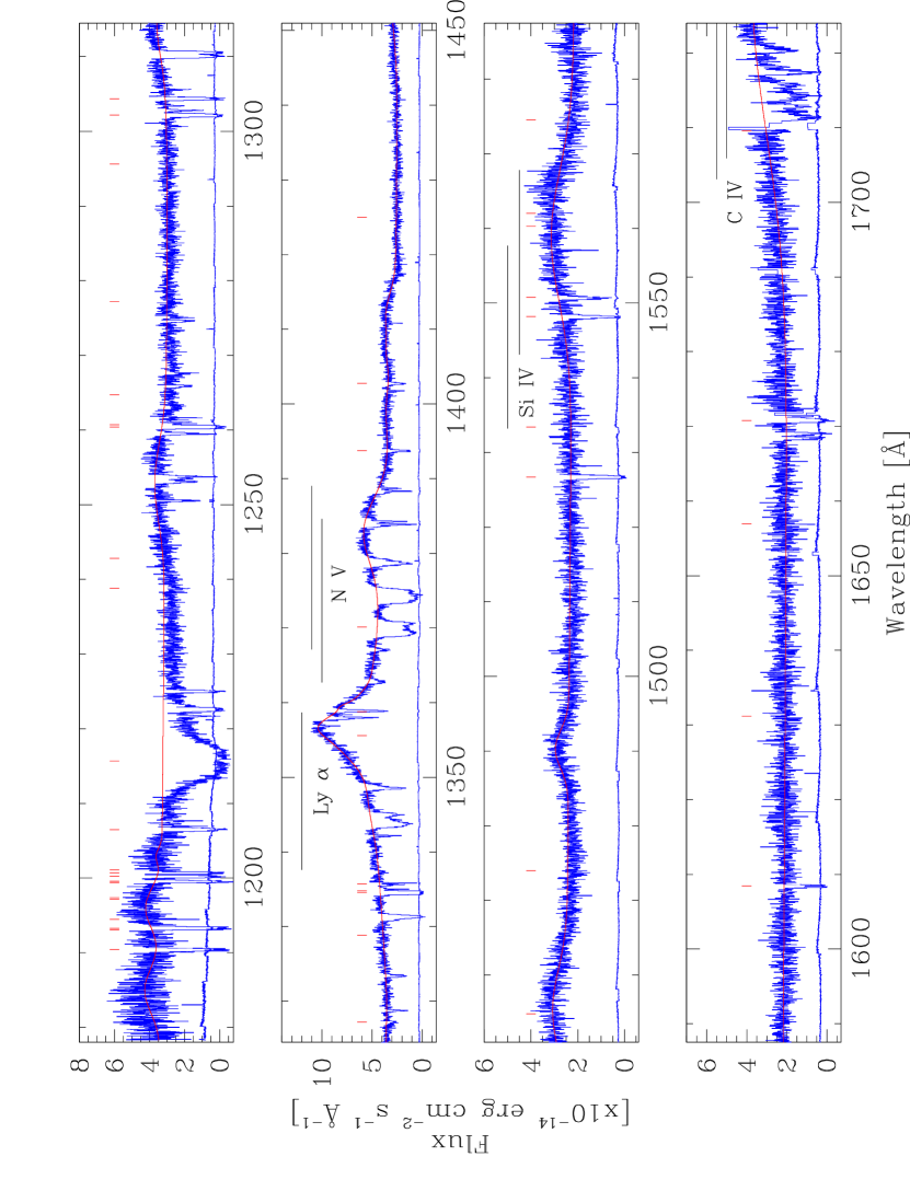
Figure 1.— Fully calibrated HST/STIS-E140M echelle spectrum of RX J$\mathbf{1230.8+0115}$: The spectrum covers the wavelength range 1178.2–1723.8 Å, with continuous coverage in the region 1178.2–1634 Å. The spectrum has been resampled and rebinned to resolution element samples to reduce noise. The lower trace in each panel is the $1\sigma$ error spectrum. The wavelength ranges covered by associated absorption are shown for Ly $\alpha$, N v $\lambda\lambda 1238.8,1242.8$, Si iv $\lambda\lambda 1393.8,1402.8$, and C iv $\lambda\lambda 1548.2,1550.7$. Vertical ticks mark the expected locations of Galactic absorption from H i, C i, C ii, C iv, N i, N v, O i, Mg i, Al ii, Si ii, Si iii, Si iv, P ii, P iii, S i, S ii, S iii, Mn ii, Fe ii, Ni ii, and Cu ii.

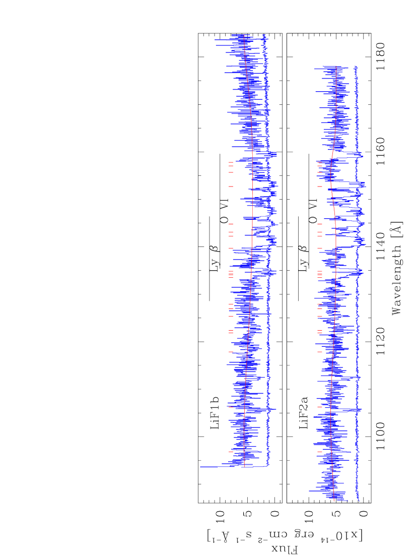
Figure 2.— Fully calibrated FUSE-LiF spectrum of RX J$\mathbf{1230.8+0115}$: In the above plot, we show spectra from the two FUSE channels (LiF1b and LiF2a) which cover the O vi $\lambda\lambda 1031.9,1037.6$ and Ly $\beta$ transitions for the associated absorbers. The spectra cover the wavelength range 1086.4–1184.8 Å. The spectrum has been resampled and rebinned to resolution element samples to reduce noise. The lower trace in each panel is the $1\sigma$ error spectrum. The wavelength ranges covered by associated absorption are shown for Ly $\beta$, and O vi $\lambda\lambda 1031.9,1037.6$. Vertical ticks mark the expected locations of Galactic absorption from C i, N i, P ii, and Fe ii.

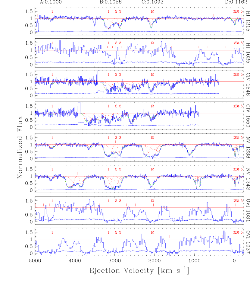
Figure 3.— Velocity Plot of Absorption Complex: The intrinsic absorption complex is detected in H i Ly $\alpha$, H i Ly $\beta$, N v $\lambda\lambda 1238.8,1242.8$, C iv $\lambda\lambda 1548.2,1550.7$, and O vi $\lambda\lambda 1031.9,1037.6$. In this plot, we transform the spectra to velocity space using $z=0.117$ as the zero-point for each of the five rest-wavelengths. The systems are labelled A,B,C, and D as described in the text with their centroid redshift. Within each system, we assign a component number. The H i Ly $\beta$, and O vi absorption are data from the FUSE LiF2a channel. The dotted curves in the STIS data (H i Ly $\alpha$, N v $\lambda\lambda 1238.8,1242.8$, C iv $\lambda\lambda 1548.2,1550.7$) show the components used to fit the absorption. For purposes of clarity, the Galactic Ni ii absorption has been removed from the N v absorption in system B.

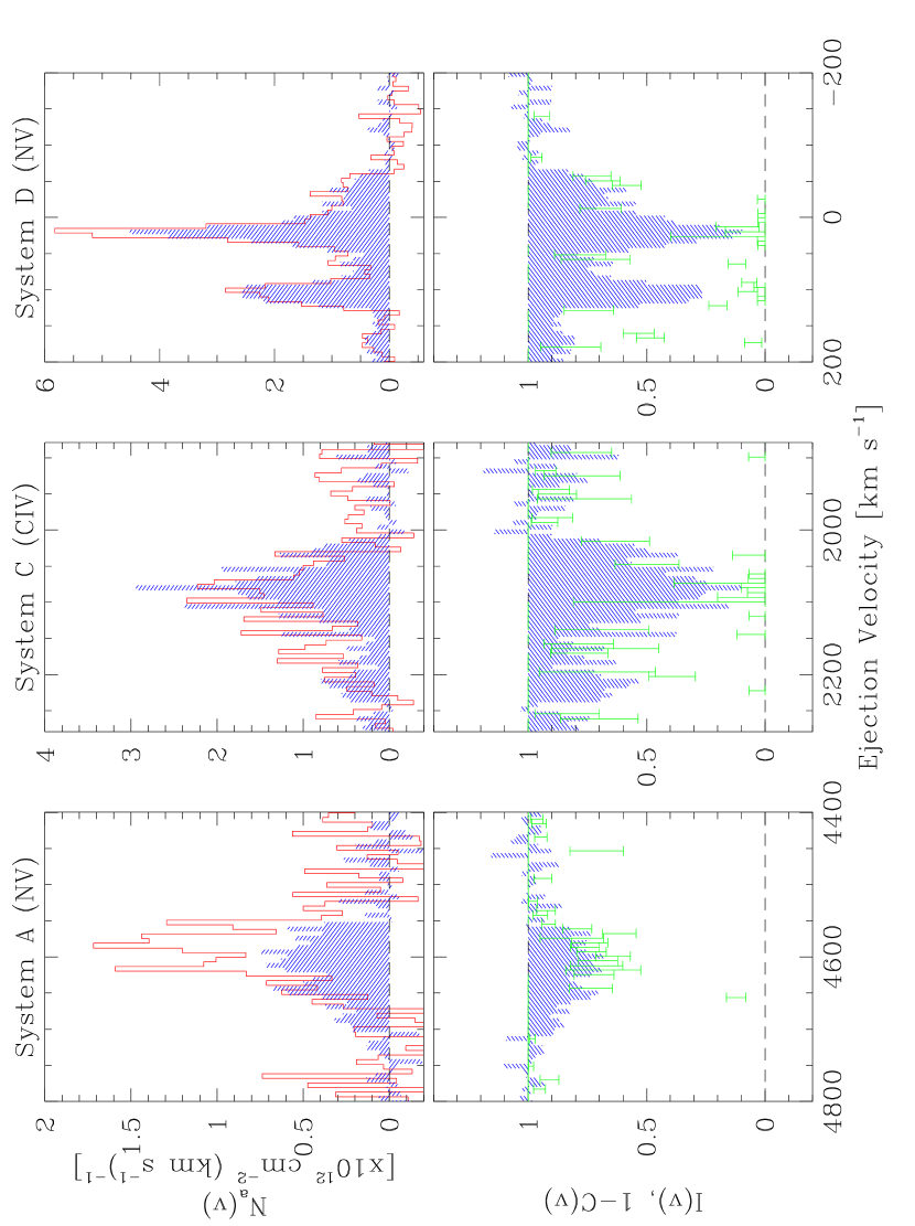
Figure 4.— Partial Coverage Plots: In the above panels, we directly invert the unblended absorption systems to test for the presence of diluted profiles. This is done for doublet from three systems: N v $\lambda\lambda 1238.8,1242.8$ for systems A (left) and D (right), and C iv $\lambda\lambda 1548.2,1550.7$ for system C (middle). The top panels show the velocity-aligned apparent column density profiles from the two transitions (stronger as shaded histogram, weaker as unshaded histogram). In the limit of fully resolved profiles, the signature of dilution is higher predicted column densities from the weaker transition. In the bottom panels we show the normalized flux from the stronger transition (shaded histogram), and directly compute the coverage fraction using eq. 2 (shown with error bars). Note that the coverage fractions are plotted on an inverted scale to show the “true” limit of saturation.

Figure 5.— Ionization Conditions of Absorbers: We plot the allowed region ($1\sigma$ confidence) of total column density $N(\mathrm{H})$ and $U$ for each component with measured or constrained C iv and N v column densities. For components B1, B2, and C2, enclosed regions are shown as solid lines. For component B3, the allowed (hatched) region continues off the figure since there is no upper constraint on the N v column density. Similarly, component A1 has only lower limits for both N v and C iv column densities propagate into a lower limit contour (dotted curve), with no upper bound.

Figure 6.— Modified Accretion-Disk/Wind Cartoon: In this modification of the “standard” accretion-disk/wind model (e.g., Murray et al., 1995; Proga et al., 2000), we propose that changes in the mass outflow rate can produce instabilities not accounted for by current numerical simulations. An instability at the base of a line-driven wind may create line-locking instabilities at the appropriate velocities. In the plot, we exaggerate the regions of the wind where locked matter may pile-up. Dark (blue) regions indicate the continuum and broad emission lines regions. All lines of sight that reach the observer are shown in light shade (light blue). To properly account for partial continuum source occultation, the wind likely flows in a mostly radial direction.

Figure 7.— Accuracy of Model-Derived Coverage Fractions and Optical Depths: In the above panels, we show the histograms of parameter differences (coverage fraction in the left panel; optical depth in the right panel) between the model (eq. 3) and the direct inversion technique. The distributions peak at zero, indicating that there is no systematic offset between the model and direct inversion.

References

- Aldcroft et al. (1994) Aldcroft, T. L., Bechtold, J., & Elvis, M. 1994, ApJS, 93, 1
- Arav et al. (2002) Arav, N., Korista, K. T., & de Kool, M. 2002, ApJ, 566, 699
- Bahcall et al. (1993) Bahcall, J. N., et al. 1993, ApJS, 87, 1
- Bahcall et al. (1996) Bahcall, J. N., et al. 1996, ApJ, 457, 19
- Barlow & Sargent (1997) Barlow, T. A., & Sargent, W. L. W. 1997, AJ, 113, 136
- Barlow et al. (1997) Barlow, T. A., Hamann, F., & Sargent, W. L. W. 1997, in ASP Conf. Ser. 128: Mass Ejection from Active Galactic Nuclei, ed. N. Arav, I. Shlosman, & R. J. Weymann (San Francisco: ASP), 13
- Becker et al. (1995) Becker, R. H., White, R. L., & Helfand, D. J. 1995, ApJ, 450, 559
- Brandt et al. (2000) Brandt, W. N., Laor, A., & Wills, B. J. 2000, ApJ, 528, 637
- Braun & Milgrom (1989) Braun, E., & Milgrom, M. 1989, ApJ, 342, 100
- Brown et al. (2002) Brown, T., et al. 2002, in HST Data Handbook, version 4.0, ed. B. Mobasher (Baltimore: STScI)
- Churchill et al. (1999) Churchill, C. W., Schneider, D. P., Schmidt, M., & Gunn, J. E. 1999, AJ, 117, 2573
- Crenshaw et al. (1998) Crenshaw, D. M., Maran, S. P., & Mushotzky, R. F. 1998, ApJ, 496, 797
- Crenshaw et al. (1999) Crenshaw, D. M., Kraemer, S. R., Boggess, A., Maran, S. P., Mushotzky, R. F., Wu, C.-C. 1999, ApJ, 516, 750
- De Kool et al. (2001) De Kool, M., Arav, N., Becker, R. H., Laurent-Muehleisen, S. A., Price, T., Korista, K. T. 2001, ApJ, 548, 609
- Dickey & Lockman (1990) Dickey, J. M., & Lockman, F. J. 1990, ARA&A, 28, 215
- Elvis (2000) Elvis, M. 2000, ApJ, 545, 63
- Ferland (2001) Ferland, G. J. 2001, Hazy, a brief introduction to Cloudy 94.00
- Foltz et al. (1987) Foltz, C. B., Weymann, R. J., Morris, S. L., & Turnshek, D. A. 1987, ApJ, 317, 450
- Foltz et al. (1988) Foltz, C. B., Chaffee, F. H., Weymann, R. J., & Anderson, S. F. 1988, in Proceedings of the QSO Absorption Line Meeting, 53
- Ganguly et al. (1999) Ganguly, R., Eracleous, M., Charlton, J. C., & Churchill, C. W. 1999, AJ, 117, 2594
- Ganguly et al. (2001a) Ganguly, R., Bond, N. A., Charlton, J. C., Eracleous, M., Brandt, W. N., & Churchill, C. W. 2001a, ApJ, 549, 133
- Ganguly et al. (2001b) Ganguly, R., Charlton, J. C., & Bond, N. A. 2001b, ApJ, 553, L101
- Ganguly (2002) Ganguly, R. 2002, in ASP Conf. Ser. 255: Mass Outflow in Active Galactic Nuclei: New Perspectives, eds. D. M. Crenshaw, S. B. Kraemer, & I. M. George (San Francisco: ASP), 111
- Ganguly et al. (2003) Ganguly, R., Sembach, K. R., & Charlton, J. C. 2003, in ASSL Conference Proceedings Vol. 281: The IGM/Galaxy Connection: The Distribution of Baryons at z=0, eds. J. L. Rosenberg & M. E. Putman (Dordrecht: Kluwer), 283
- Gray (1992) Gray, D. F. 1992, The Observation and Analysis Of Stellar Photospheres (2 ed.) (Cambridge University Press)
- Hamann et al. (1995) Hamann, F., Barlow, T. A., Beaver, E. A., Burbidge, E. M., Cohen, R. D., Junkkarinen, V., & Lyons, R. 1995, ApJ, 443, 606
- Hamann et al. (1997a) Hamann, F., Barlow, T. A., Junkkarinen, V., & Burbidge, E. M. 1997a, ApJ, 478, 80
- Hamann et al. (1997b) Hamann, F., Barlow, T. A., & Junkkarinen, V. 1997b, ApJ, 478, 87
- Hamann et al. (2000) Hamann, F. W., Netzer, H., & Shields, J. C. 2000, ApJ, 536, 101
- Impey et al. (1999) Impey, C. D., Petry, C. E., & Flint, K. P. 1999, ApJ, 524, 536
- Jannuzi et al. (1998) Jannuzi, B. T., et al. 1998, ApJS, 118, 1
- Kaspi et al. (2000) Kaspi, S. Smith, P. S., Netzer, H., Maoz, D., Jannuzi, B. T., & Giveon, U. 2000, ApJ, 533, 631
- Korista et al. (1993) Korista, K. T., Voit, G. M., Morris, S. L., Weymann, R. J. 1993, ApJS, 88, 357
- Kraemer et al. (2001) Kraemer, S. B., et al. 2001, ApJ, 551, 671
- Lanzetta et al. (1987) Lanzetta, K. M., Wolfe, A. M., & Turnshek, D. A. 1987, ApJ, 322, 739
- Laor et al. (1997) Laor, A., Fiore, F., Elvis, M., Wilkes, B. J., & McDowell, J. C. 1997, ApJ, 477, 93
- Mathur et al. (1995) Mathur, S., Elvis, M., & Wilkes, B. 1995, ApJ, 452, 230
- Milne (1926) Milne, E. A. 1926, MNRAS, 86, 459
- Misawa et al. (2003) Misawa, T., Yamada, T.,Takada-Hidai, M., Wang, Y., Kashikawa, N., Iye, M., & Tanaka, I. 2003, AJ, 125, 1336
- Møller & Jakobsen (1987) Møller, P., & Jakobsen, P. 1987, ApJ, 320, L75
- Murray et al. (1995) Murray, N., Chiang, J., Grossman, S. A., & Voit, G. M. 1995, ApJ, 451, 498
- Penton et al. (2000a) Penton, S. V., Shull, J. M., & Stocke, J. T. 2000a, ApJ, 544, 150
- Penton et al. (2000b) Penton, S. V., Stocke, J. T., & Shull, J. M. 2000b, ApJS, 130, 121
- Press et al. (1992) Press, W. H., Teukolsky, S. A., Vetterling, W. T., & Flannery, B. P. 1992, Numerical recipes in C. The art of scientific computing (Cambridge: Cambridge University Press, c1922, 2nd ed.)
- Proga et al. (2000) Proga, D., Stone, J. M., & Kallman, T. R. 2000, ApJ, 543, 686
- Read et al. (1998) Read, M. A., Miller, L., & Hasinger, G. 1998, A&A, 335, 121
- Richards et al. (2002a) Richards, G. T., Gregg, M. D., Becker, R. H., & White, R. L. 2002a, ApJ, 567, L13
- Richards et al. (2002b) Richards, G. T., Vanden Berk, D. E., Reichard, T. A., Hall, P. B., Schneider, D. P., SubbaRao, M., Thakar, A. R., & York, D. G. 2002b, AJ, 124, 1
- Richards et al. (1999) Richards, G. T., York, D. G., Yanny, B., Kollgaard, R. I., Laurent–Muehleisen, S. A., & vanden Berk, D. E. 1999, ApJ, 513, 576
- Rosenberg et al. (2003) Rosenberg, J. L., Ganguly, R., Giroux, M. L., & Stocke, J. T. 2003, ApJ, in press
- Runacres & Owocki (2002) Runacres, M. C., & Owocki, S. P. 2002, A&A, 381, 1015
- Savage & Sembach (1991) Savage, B. D. & Sembach, K. R. 1991, ApJ, 379, 245
- Scargle (1973) Scargle, J. D. 1973, ApJ, 179, 705
- Schneider et al. (1993) Schneider, D. P., et al. 1993, ApJS, 87, 45
- Shakura & Sunyaev (1973) Shakura, N. I., & Sunyaev, R. A. 1973, A&A, 24, 337
- Sutherland & Doptia (1993) Sutherland, R. S., & Dopita, M. A. 1993, ApJS, 88, 253
- Turnshek (1988) Turnshek, D. A. 1988, in QSO Absorption Lines; Probing the Universe; Proceedings of the QSO Absorption Line Meeting, ed. J. C. Blades, D. A. Turnshek, & C. A. Norman (Cambridge: Cambridge University Press), 17