The Impact of Pollution on Stellar Evolution Models

Abstract

An approach is introduced for incorporating the concept of stellar pollution into stellar evolution models. The approach involves enhancing the metal content of the surface layers of stellar models. In addition, the surface layers of stars in the mass range of $0.5-2.0\,\mathrm{M}_{\odot}$ are mixed to an artificial depth motivated by observations of lithium abundance. The behavior of polluted stellar evolution models is explored assuming the pollution occurs after the star has left the fully convective pre main sequence phase. Stellar models polluted with a few Earth masses ($\mathrm{M}_{\oplus}$) of iron are significantly hotter than stars of the same mass with an equivalent bulk metallicity. Polluted stellar evolution models can successfully reproduce the metal-rich, parent star $\tau$ Bootis and suggest a slightly lower mass than standard evolution models. Finally, the possibility that stars in the Hyades open cluster have accreted an average of $0.5\,\mathrm{M}_{\oplus}$ of iron is explored. The results indicate that it is not possible to rule out stellar pollution on this scale from the scatter of Hyades stars on a color-magnitude diagram. The small amount of scatter in the observational data set does rule out pollution on the order of $\sim 1.5\,\mathrm{M}_{\oplus}$ of iron. Pollution effects at the low level of $0.5\,\mathrm{M}_{\oplus}$ of iron do not produce substantial changes in a star’s evolution.

1 Introduction

The discoveries of dozens of giant planets in orbits with semi-major axes less than 1 AU (for a complete listing see www.exoplanets.org), which began in 1995 (Mayor & Queloz, 1995), posed a problem for planet formation theories. Such theories indicate that giant planets ought to form in orbits with semi-major axes greater than 1 AU. However, through interactions with other planets and the protoplanetary disk it is possible for these planets to migrate inward until they reach a stable orbit (Lin & Shigeru, 1997). The inward migration can sweep material in the disk onto the surface of the star. Gonzalez (1997) pointed out that if the accreted material is metal-rich then stars with planets (SWPs) will exhibit enhanced metallicity, a concept referred to as “stellar pollution”.

The case has been made in recent years that SWPs are metal rich, for example Laws & Gonzalez (2002). The two main explanations for these stars to be metal-rich are a high intrinsic metallicity and the accretion of $\sim$5 $\mathrm{M}_{\oplus}$ of iron from the protoplanetary disk, for a more complete discussion see Murray & Chaboyer (2002).

Based upon the apparent deficiency of heavy elements in the asteroid belt, and considerations of orbital dynamics in the early solar system, Murray et al. (2001) found that the formation of Jupiter likely led to the accretion of $\sim$0.5 $\mathrm{M}_{\oplus}$ of iron onto the Sun. Their analysis of the correlations between [Fe/H]–age–mass in local field stars lead Murray et al. (2001) to suggest that stellar pollution effects in the solar neighborhood appear to be quite common at a similar level. Using a Monte Carlo approach they estimate that field stars have accreted an average of $\sim$0.5 $\mathrm{M}_{\oplus}$ of iron with standard deviation equal to half the mean. Hence, Murray et al. (2001) suggest that most protoplanetary disks are similar to that of the Sun and not the stars in the SWPs sample.

In a paper on modeling the evolution of SWPs, Ford et al. (1999) discuss the need for stellar evolution models which have enhanced surface metallicities relative to the interiors. The authors briefly explain their approach to the problem which involves increasing the metallicity of the surface convection zone and/or decreasing the interior metallicity, and discuss the impact of such models on the Sun and a few SWPs. The main thrust of the paper is, however, modeling SWPs with standard stellar evolution models.

In this paper, stellar evolution models are presented which allow for the addition of metal-rich material to the surface. The behavior of these models is compared standard stellar evolution models. The modifications made to standard stellar evolution models are explained in $\S$2. The basic impact of these changes on the evolution of a star is presented $\S$3. In $\S$4 the metal-rich parent star $\tau$ Bootis is modeled with both polluted and unpolluted models and the results are compared. In $\S$5 polluted model isochrones are compared to observational data on the Hyades; the likelihood that the Hyades stars have experienced low-level pollution is discussed. The attempt to create polluted stellar evolution models is summarized in $\S$6.

2 Stellar Models

Stellar evolution models were constructed using the Dartmouth stellar evolution code (Chaboyer et al., 2001). Helium and heavy element diffusion are included using Thoul et al. (1994). All models use a solar calibrated mixing length $\alpha$ = 1.75. The models were evolved from pre main sequence, fully convective polytropes to the main sequence turnoff in $\sim$800 time steps and include overshooting of the surface convection zone.

Murray et al. (2001) suggest that we may model the depletion of lithium from the photosphere by introducing a convective overshoot to the surface convection zone. They present a model for the mass of the surface mixed layer (SML) as a function of stellar mass and [Fe/H] which has been implemented in the code for this work. Each time the code calls for the surface convection zone to be mixed we calculate the mass of the SML and mix down to its base. For a plot of SML mass as a function of stellar mass, see Figure 2 of Murray et al. (2001).

In the literature on stellar pollution the amount of accreted material is often referred to in Earth masses ($\mathrm{M}_{\oplus}$) of iron. We shall follow this convention throughout. Following arguments made by Murray et al. (2001), protoplanetary material is roughly 20% iron by mass. Note that we are essentially changing the mass fraction of heavy elements (Z) in the models and the accretion of 1 $\mathrm{M}_{\oplus}$ of iron corresponds to the addition of 5 $\mathrm{M}_{\oplus}$ of Z.

Stars which accret rocky material will experience an increase in heavy element composition in the outer layers. Our approach is to rescale the composition of the SML without altering its mass. Starting with an amount of iron, we take the ratio of the mass of rocky material to the mass of the SML ($\mathrm{Z_{rock}}$) and add this to the initial mass fraction of metals ($\mathrm{Z_{i}}$). The new mass fraction of metals is

$$Z_{f}=Z_{i}+Z_{rock}$$ (1)

A new heavy element mass fraction is calculated and the abundances of hydrogen (X) and helium (Y) are adjusted. We rescale X and Y as follows

$$\frac{X_{f}}{X_{i}}=1-\frac{Z_{rock}}{1-Z_{i}}$$ (2)

$$\frac{Y_{f}}{Y_{i}}=1-\frac{Z_{rock}}{1-Z_{i}}$$ (3)

The $i$- and $f$-subscripts refer to initial and final compositions, respectively.

In models which accrete more than about $1\,\mathrm{M}_{\oplus}$ of iron we found it necessary to increase the metallicity over multiple time steps. Spreading the pollution over several time steps allows us to avoid the problems which occur when the conditions in the model change too quickly for the code to adjust. In addition, it is more in line with current theories which describe the time scales of stellar pollution as taking place over tens of millions of years. Neither altering the time scale nor changing the exact age at which rocky material is accreted (after the zero-age main sequence, ZAMS) has a significant impact on evolution. Unless otherwise noted, we begin to add the rocky material when the model reaches the ZAMS. Since all stars considered metal rich compared to the Sun we rescale Y and Z (from Solar values) in the ratio $\Delta$Y/$\Delta$Z = 2 (Chaboyer et al., 1999).

Finally, to calculate [Fe/H] it is sufficient to use [Fe/H]=log($mathrm{Z_{*}/Z_{\odot}}$) since the relative change in X is insignificant compared to the relative change in Z. However, this assumes the star in question has the same abundance of iron as the Sun. The accreted material is roughly 20% iron by mass, while the Sun is only about 0.14% iron by mass (iron comprises 7.3% of $\mathrm{Z_{\odot}}$ by mass, and $\mathrm{Z_{\odot}}$=0.019). We account for this difference by introducing a factor to the [Fe/H] formula which accounts for the increased abundance of iron on the surface of the star.

$$\left[\frac{Fe}{H}\right]=log\left(\frac{Z_{*}}{Z_{\odot}}\right)+log\left(\frac{M_{P}(Fe)+M_{SML}(Fe)}{M_{SML}(Fe)}\right)$$ (4)

Where $\mathrm{M_{P}}$(Fe) is the mass of iron in the polluting material and $\mathrm{M_{SML}}$(Fe) is the mass of iron in the SML.

3 Basic Results

The most significant impact of stellar pollution on the evolution of star is the difference in effective temperature. Given two main sequence stars of similar mass, age, and surface metallicity a polluted star will have a higher effective temperature than an unpolluted star (for a specific example see $\S$4).

The altered behavior can be interpreted as follows: the unpolluted model has a higher mass fraction of heavy elements in the deep interior (below the SML). This leads to a higher opacity in the deep interior of the unpolluted model, making it more difficult for energy to flow outward. The unpolluted model is thus physically larger and cooler than the polluted model.

The effect of adding a given amount of iron to a star decreases with SML mass because mixing the polluting material over a larger region dilutes the effect.

4 $\tau$ Bootis

Recent evidence that SWPs are metal-rich (Laws & Gonzalez, 2002) compared to a sample of field stars lends support to the concept that these stars have accreted metal-rich material before the planetary system reached equilibrium. If the accretion occurred after the star left the pre main sequence convective phase the effects should be noticeable in the form of high metallicity.

$\tau$ Bootis has a short-period, giant planet. It also has a high metallicity, [Fe/H]=0.32$\pm$0.06 (Gonzalez & Laws, 2000). To illustrate the effects stellar pollution may have when stellar models are used to infer properties of real stars, observational data for $\tau$ Boo was fitted by standard and polluted models.

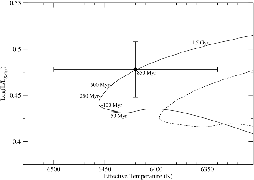
Figure 1: H-R diagram showing polluted (solid line) and unpolluted (dashed line) models with M = 1.36 $\mathrm{M}_{\odot}$. Both models have the same [Fe/H] at the surface. The error bars represent observationally derived values for $\tau$ Boo. The polluted model received 2 $\mathrm{M}_{\oplus}$ of iron at the ZAMS.

A series of polluted models was constructed with masses between 1.30 and 1.40 $\mathrm{M}_{\odot}$ adding 1-5 $\mathrm{M}_{\oplus}$ of iron when the model reaches the ZAMS. Figure 1 shows the evolutionary tracks of two 1.36 $\mathrm{M}_{\odot}$ stellar models. The solid line is a model polluted with 2 $\mathrm{M}_{\oplus}$ of iron. The dashed line is an unpolluted model with bulk metallicity chosen to match the surface metallicity of the polluted model. The polluted model is marked at several points to show how the model evolves with time. The unpolluted model evolves in the same manner.

Table 1: $\tau$ Boo Model Results

Mass ($\mathrm{M}_{\odot}$)	Log(L/$\mathrm{L_{\odot}}$)	$\mathrm{T_{eff}}$ (K)	[Fe/H]	$\mathrm{Z_{init}}$	$\mathrm{Z_{rock}}$ ($\mathrm{M}_{\oplus}$ Fe)	Age (Gyr)
Observational Data
$\cdots$	0.478${+0.030\atop-0.032}$	6420$\pm$80	0.32$\pm$0.06	$\cdots$	$\cdots$	$\cdots$
Polluted Models
1.380	0.486	6435	0.364	0.039	1	0.66
1.360	0.478	6420	0.362	0.035	2	0.85
1.345	0.500	6435	0.345	0.030	3	1.18
1.330	0.476	6415	0.329	0.028	3	1.20
1.320	0.478	6420	0.340	0.025	4	1.35
1.300	0.478	6420	0.325	0.023	4	1.54
Unpolluted Models
1.400	0.497	6450	0.375	0.043	$\cdots$	0.51
1.380	0.478	6420	0.335	0.040	$\cdots$	0.64
1.360	0.479	6430	0.278	0.035	$\cdots$	0.85
1.345	0.490	6435	0.275	0.035	$\cdots$	0.98

Table 1 contains a small sample of polluted models with luminosities, temperatures, and ages at closest approach to the observational data. For comparison we include models constructed using the same evolution code but which have not been polluted.

The data in Table 1 show that, for a given mass, the polluted models are slightly older than the unpolluted models: from a few percent at the high mass end (around 1.40 $\mathrm{M}_{\odot}$) up to 20% at the low mass end (1.34 $\mathrm{M}_{\odot}$). The polluted models have a best fit mass which is 0.02 - 0.03 $\mathrm{M}_{\odot}$ lower than the best fit from the unpolluted models. The purpose of this table is only to illustrate the general trends which pollution has on stellar models, and not to constrain the stellar mass of, or amount of pollution, experienced by, $\tau$ Boo.

5 The Hyades

Murray et al. (2001) estimate that stars in the solar neighborhood have accreted 0.5$\pm$0.25 $\mathrm{M}_{\oplus}$ of iron. The sample used to make this estimate was comprised of field stars which have a broad range of ages and bulk metallicities. The variation in age and metallicity of the sample, along with the fact that younger stars tend to be more metal-rich than older stars, complicated the analysis of Murray et al. (2001).

Stars in the Hyades are likely to have formed at the same time from material of the same composition. As a result, Hyades stars are likely to yield better constraints than field stars on stellar pollution. The relatively young age of stars in the Hyades, combined with a uniform composition, should imply a tight main sequence. However, planet formation and accretion of metal-rich material will vary from one star to another which will cause scatter in the color-magnitude diagram (CMD).

Quillen (2002) proposes that the scatter of Hyades stars about a theoretical isochrone can be used to limit the level of pollution experienced by Hyades stars. Quillen (2002) did not have access to polluted stellar evolution models, and so based her proposal on some plausible assumptions that the effects of stellar pollution would have on the evolution of stars. With the modified evolution code presented in this paper it is possible to directly test Quillen’s proposal.

As a preliminary test, three isochrones were constructed with varying levels of pollution. Each isochrone consists of models ranging in mass from 0.6 to 1.8 $\mathrm{M}_{\odot}$ in steps of 0.05 $\mathrm{M}_{\odot}$. Each model begins on the pre main sequence, receives the polluting material at about 150 Myr (at which point all models have reached or passed the ZAMS), and is evolved to 650 Myr. Uncertainty in the final age of the isochrones by $\pm$50 Myr alters the scatter by an amount roughly an order of magnitude below the scatter due to pollution effects.

The models in each isochrone have a common initial $Z=0.024$ leading to $<$[Fe/H]$>\,\simeq\,$0.13 in accord with Boesgaard & Friel (1990) who find $<$[Fe/H]$>$ = 0.127$\pm$0.022 in the range of 6000 - 7000 K. In the “mean” polluted isochrone, models are polluted with 0.5 $\mathrm{M}_{\oplus}$ of iron. The other two isochrones correspond to pollution amounts of $2\,\sigma$ above and below the mean, respectively 1.0 and 0.0 $\mathrm{M}_{\oplus}$ of iron.

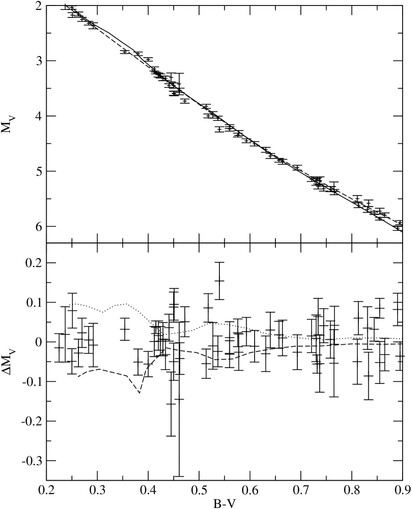
Figure 2: $Top\,Panel$–A CMD of the Hyades sample with the mean polluted isochrone (solid line) and LOWESS fit (dashed line) superimposed. $Bottom\,Panel$–A scatter plot in $\Delta\mathrm{M_{V}}$ of the Hyades sample about the LOWESS fit. Superimposed are the differences between the $2\,\sigma$ isochrones and the mean isochrone. (dashed line: $+2\,\sigma$; dotted line: $-2\,\sigma$).

The top panel in Figure 2 is a CMD showing the main sequence from 0.6 – 1.8 $\mathrm{M}_{\odot}$ of the Hipparcos Hyades sample of de Bruijne et al. (2001) (also used by Quillen (2002) ). Buser & Kurucz (1992) color tables were used to convert the models from luminosity and effective temperature to $\mathrm{M_{V}}$ and B–V. In addition, the CMD plot includes the mean polluted isochrone and a fit to the data made using the LOWESS (Locally Weighted Regression) technique (Cleveland, 1979; Gebhardt et al., 1994, 1995). In the plot the dashed line is the LOWESS fit and the solid line is the mean isochrone. The LOWESS fit is weighted by the the local points, and represents the best fit to the data that is possible with a single line.

The bottom panel of Figure 2 shows the scatter of the Hyades sample about the LOWESS fit. Superimposed are the differences between the $2\,\sigma$ isochrones and the mean isochrone. The difference between the mean and $+2\,\sigma$ isochrone is represented by the dashed line; the difference between the mean and the $-2\,\sigma$ isochrone is represented by the dotted line. Note that the dispersion of the data points is smaller than that predicted by the $\pm 2\,\sigma$ models, showing that the dispersion predicted by the stellar pollution models is not ruled out by the data.

The LOWESS technique is used to fit the Hipparcos Hyades sample because the mean polluted isochrone diverges slightly from the main sequence for $\mathrm{B-V}$ greater than $\sim$0.65 mag. This difference between the models and the data is likely due to problems with the treatment of convection, or in the color calibration of the models. We are not interested in studying this problem in this paper, rather the goal is to compare the scatter in the Hyades stars about a smooth main sequence to the predicted scatter caused by pollution. The LOWESS fit allows a comparison between the observed scatter and the theoretical prediction which is not hampered by large scale errors introduced by the color conversion and/or treatment of convection. In general, the theoretical isochrone is a reasonable fit to the data, with the the only consistent deviation between the LOWESS fit and the mean polluted isochrone occurring for $\mathrm{B-V}\geq 0.65$ mag.

The fit of the mean polluted isochrone to the observational data has a reduced $\chi^{2}$ of $\sim$3.3 and the LOWESS fit has a reduced $\chi^{2}$ of 2.1. The mean polluted isochrone has the lowest $\chi^{2}$ of all the isochrones constructed and is therefore the standard. The LOWESS fit is the best is possible single line fit to the data, and the large value of $\chi^{2}$ implies that their is an inherent dispersion in the data.

As a more stringent test, the method of Gebhardt et al. (1994, 1995) for determining the velocity dispersion as a function of radius within a globular cluster has been adapted to study the scatter in the CMD. In this method, the value of the error bar for each star in the Hyades sample is removed in quadrature from the absolute value of $\Delta\mathrm{M_{V}}$ (scatter) value of that star. The square root of the resulting value is the $\mathrm{M_{V}}$ dispersion, analogous to the velocity dispersion in the globular cluster studies of Gebhardt et al. (1994, 1995). If the size of the error bar is larger than the absolute value of $\Delta\mathrm{M_{V}}$ for a given data point, the $\mathrm{M_{V}}$ dispersion is set to zero for that point. The LOWESS fit is then determined for $\Delta\mathrm{M_{V}}$ as a function of B V. This produces “dispersion profile” for the Hyades sample. Note that the dispersion is a non-negative quantity, any information about the scatter being above or below the mean isochrone is lost.

The final step is to estimate the error in the derived dispersion profile. This is done in a manner somewhat analogous to the standard bootstrap re-sampling technique for error analysis. In particular, for each data point one randomly selects a new value for $\mathrm{M_{V}}$ using a Gaussian distribution, with a mean equal to the original value of $\mathrm{M_{V}}$ and a one-$\sigma$ width equal to the quoted one-sigma error in the data point. The process is performed one thousand times for each star and a mean dispersion profile with confidence bands is calculated from the results.

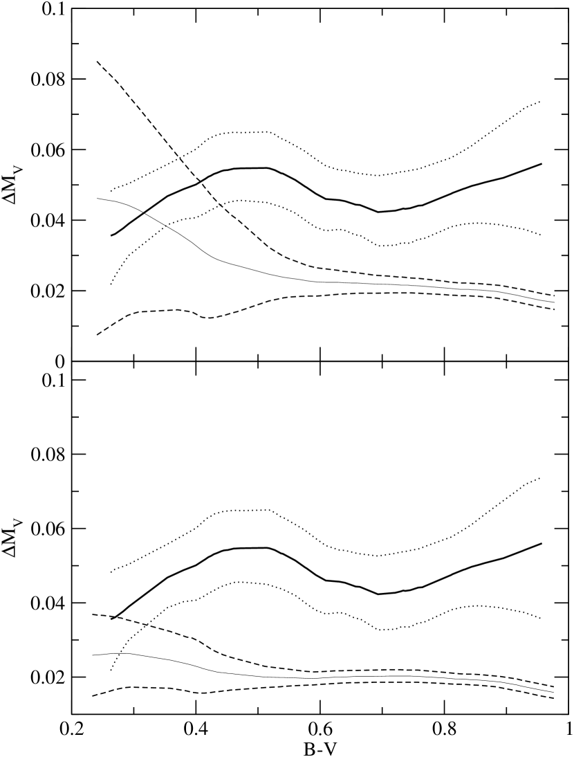
Figure 3: $Top\,Panel$–Comparison of the dispersion in the Hyades sample (thick line) and the average of the mock data sets with mean pollution of 1.0 $\mathrm{M}_{\oplus}$ (thin line). 90% confidence bands are drawn for the dispersion in the data (dotted lines) and the mock data sets (dashed lines). $Bottom\,Panel$–Same as the top panel but for the 0.5 $\mathrm{M}_{\oplus}$ case.

Having obtained the dispersion profile for the Hyades data, it is necessary to put the theoretical prediction in a similar form for comparison. Using the mean polluted isochrone as a guide, the mass of each star with $0.2\leq\mathrm{B-V}\leq 1.0$ in the Hyades sample was determined. Stellar models with these particular values of mass were evolved 1000 times, where each of the stellar evolution models had a random amount of stellar pollution added to it at 150 Myr. The amount of the polluting material was drawn from a Gaussian distribution with standard deviation equal to half the mean. This is done for two cases, means equal to 0.5 and 1.0 $\mathrm{M}_{\oplus}$ of iron.

The result of this simulation is a set of 2000 theoretical CMDs, where each CMD contains the same number of data points as the Hyades data set, but for each each of the stars in the CMD has been polluted by a varying amount. To compare with the dispersion profile in the data, the individual theoretical CMD is treated as a “mock” data set and put through the exact same procedure as the real data set to generate a dispersion profile of $\mathrm{M_{V}}$ as a function of B V. This was done each of the 2000 theoretical CMDs, first for 1000 CMDs which had a mean amount of pollution equal to 0.5 $\mathrm{M}_{\oplus}$ of iron and then for the 1000 CMDs with a mean pollution of 1.0 $\mathrm{M}_{\oplus}$ of iron.

Figure 3 is a plot of the dispersion in the data and in the averaged mock data sets. In the both panels, the thick line is the mean dispersion in the data and the thin line is the mean dispersion in the averaged mock data sets. The 1.0 $\mathrm{M}_{\oplus}$ case is the top panel; the 0.5 $\mathrm{M}_{\oplus}$ case is the bottom panel. In each panel, 90% confidence bands are drawn about the mean dispersion in the Hyades data (dotted lines) and the averaged mock data sets (dashed lines). From Figure 3 it is clear that neither the 0.5 nor the 1.0 $\mathrm{M}_{\oplus}$ case is ruled out by the observed dispersion in the Hyades data at the 90% confidence level. However, looking at the trends apparent in these two cases, it is clear that pollution at the mean level of $\sim$1.5 $\mathrm{M}_{\oplus}$ of iron is ruled out by the data.

6 Conclusions

Stars with giant planets in tight orbits, such as $\tau$ Boo, are likely to have accreted $\sim$5 $\mathrm{M}_{\oplus}$ of iron (Murray & Chaboyer, 2002). A method is presented for modifying standard stellar evolution models to realistically account for this stellar pollution effects. Such polluted stars will exhibit a significantly hotter surface than stars of similar mass and age with a correspondingly high bulk metallicity. Polluted stellar evolution models may prove useful in studying the evolution of stars which prove difficult for standard stellar evolution models.

On the other hand, most stars in the solar neighborhood have not been observed to have giant planets, and appear to have accreted an average of 0.5 $\mathrm{M}_{\oplus}$ of iron (Murray et al., 2001). At such a low level, pollution effects in the CMD are found to be very small. As an example, we look at pollution effects in the Hyades open cluster. Stars in the Hyades all formed from the same material at roughly the same time. At 650 Myr the stars we have chosen are all on the main sequence and so past the era when pollution would have occurred. Monte Carlo simulations show that the dispersion in $\Delta\mathrm{M_{V}}$ of the Hyades about a polluted isochrone is consistent with the observed data, assuming that the pollution in the Hyades is at a similar level to the field star sample. However, if the level of pollution in the Hyades were a factor of 3 or more greater than that in the field stars, the analysis performed would be able to rule it out. We are currently investigating the mass-[Fe/H] relationship in the Hyades to see if this data can put stronger constraints on stellar pollution.

References

- Boesgaard & Friel (1990) Boesgard, A. M., & Friel, E. D. 1990, ApJ, 351, 467
- Buser & Kurucz (1992) Buser, R. & Kurucz, R. L. 1992, A&A, 264, 557
- Chaboyer et al. (2001) Chaboyer, B., Fenton, W. H., Nelan, J. E., Patnaude, D. J., & Simon, F. E. 2001, ApJ, 562, 521
- Chaboyer et al. (1999) Chaboyer, B., Green, E. M., & Liebert, J. 1999, AJ, 117, 1360
- Cleveland (1979) Cleveland, W. S. 1979, J. Am. Stat. Assoc., 74, 829
- de Bruijne et al. (2001) de Bruijne, J. H. J., Hoogerwerf, R., & de Zeeuw, P. T. 2001, A&A, 367, 111
- Ford et al. (1999) Ford, E. B., Rasio, F. A., & Sills, A. 1999, ApJ, 514, 411
- Gebhardt et al. (1994) Gebhardt, K., Pryor, C., Williams, T. B., & Hesser, J. E. 1994, AJ, 107, 2067
- Gebhardt et al. (1995) Gebhardt, K., Pryor, C., Williams, T. B., & Hesser, J. E. 1995, AJ, 110, 1699
- Gonzalez (1997) Gonzalez, G. 1997, MNRAS, 285, 403
- Gonzalez & Laws (2000) Gonzalez, G., & Laws, C. 2000, AJ, 119, 390
- Laws & Gonzalez (2002) Laws, C. & Gonzalez, G. 2002, AAS Meeting 201, #24.01
- Lin & Shigeru (1997) Lin, D. N. C. & Shigeru, I. 1997, ApJ, 477, 781
- Mayor & Queloz (1995) Mayor, M. & Queloz, D. 1995, Nature, 378, 355
- Murray & Chaboyer (2002) Murray, N., & Chaboyer, B. 2002, ApJ, 493, 222
- Murray et al. (2001) Murray, N., Chaboyer, B., Arras, P., Hansen, B., & Noyes, R. W. 2001, ApJ, 555, 801
- Quillen (2002) Quillen, A. C. 2002, AJ, 124, 400
- Thoul et al. (1994) Thoul, A. A., Bahcall, J. N., Loeb, A. 1994, ApJ, 421, 828