Searching for non-Gaussianity in the VSA data

Abstract

We have tested Very Small Array (VSA) observations of three regions of sky for the presence of non-Gaussianity, using high-order cumulants, Minkowski functionals, a wavelet-based test and a Bayesian joint power spectrum/non-Gaussianity analysis. We find the data from two regions to be consistent with Gaussianity. In the third region, we obtain a 96.7% detection of non-Gaussianity using the wavelet test. We perform simulations to characterise the tests, and conclude that this is consistent with expected residual point source contamination. There is therefore no evidence that this detection is of cosmological origin. Our simulations show that the tests would be sensitive to any residual point sources above the data’s source subtraction level of 20 mJy. The tests are also sensitive to cosmic string networks at an rms fluctuation level of $105~{}\mu K$ (i.e. equivalent to the best-fit observed value). They are not sensitive to string-induced fluctuations if an equal rms of Gaussian CDM fluctuations is added, thereby reducing the fluctuations due to the strings network to $74~{}\mu K$ rms . We especially highlight the usefulness of non-Gaussianity testing in eliminating systematic effects from our data.

1 Introduction

The search for non-Gaussianity in the anisotropies of the cosmic microwave background (CMB) radiation is of major importance to modern cosmology. Different fundamental theories of structure formation predict markedly different non-Gaussian CMB signatures, making the quantification of any such signatures a powerful discriminator between these possibilities. Measurements of the CMB angular power spectrum have now ruled out the classic non-Gaussian example of topological defects as the primary method of generating CMB anisotropy, although the possibility of a sub-dominant contribution remains. Recent work on different varieties of the inflationary paradigm (e.g. Peebles, 1999; Wang & Kamionkowski, 2000; Bartolo & Liddle, 2002) has shown that different forms of inflation can also be distinguished by the characterisation of any non-Gaussianity present in the CMB.

There are other very good reasons to search for non-Gaussianity in the CMB. Much of CMB cosmology centres on the accurate determination of the angular power spectrum. If the CMB fluctuations form a Gaussian random field, then the power spectrum completely characterises its statistical properties. Therefore, the detection of any non-Gaussianity would indicate that there is further information to be gathered. It is also the case that, with one exception (Rocha et al., 2001), all power spectrum analyses of CMB data assume the data to be Gaussian. As with any assumption, this must be tested if we are to have confidence in the results.

There is also the consideration of contamination of CMB data sets. Extragalactic sources, Sunyaev-Z’eldovich decrements and the various Galactic foregrounds all play their part in contaminating the CMB. Moreover, they all introduce non-Gaussianity into the data, making non-Gaussianity testing an excellent way to identify their presence. Furthermore, data contamination can occur other than by the telescope seeing something unwanted in the sky. Systematic effects are invariably an issue. The detection of non-Gaussianity in the COBE data by Ferreira et al. (1998) was traced to such an effect (Banday et al., 2000) and, in general, non-Gaussianity testing can be extremely useful in identifying and removing systematics.

As a consequence of the many-fold importance of non-Gaussianity testing to CMB cosmology, many different techniques have been developed to investigate it (see e.g. Ferreira et al., 1997; Hobson et al., 1999; Rocha et al., 2001; Verde & Heavens, 2001; Hansen et al., 2002; Chiang et al., 2002; Aghanim et al., 2003). A number of techniques have also been applied to the data from various CMB instruments over the last few years (see e.g. Wu et al., 2001; Polenta et al., 2002; Chiang et al., 2003; Komatsu et al., 2003; Troia et al., 2003; Santos et al., 2003) These analyses have shown the practical application of non-Gaussianity testing, particularly the importance of robust Monte Carlo simulation for determining the significance level of any result.

In this paper we present the results of applying a selection of non-Gaussianity tests to the VSA data set first presented in its entirety in Grainge et al. (2003) (Paper V hereafter) and Slosar et al. (2003) (Paper VI hereafter). Results from the VSA in its compact configuration have already been presented in Watson et al. (2003), Taylor et al. (2003), Scott et al. (2003), and Rubiño-Martin et al. (2003), (hereafter Papers I - IV respectively).

2 Interferometric observations of the CMB

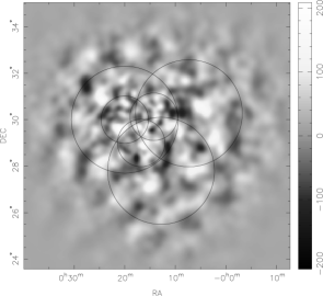
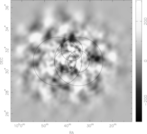
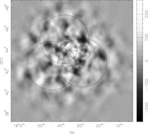
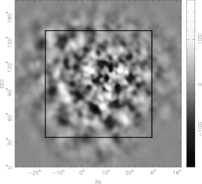
Figure 1: Top left, top right and bottom left: The VSA1, VSA2 and VSA3 mosaics. The maps are produced using a MEM algorithm. The circles denote the FWHM of the primary beams of each of the individual pointings. Bottom right: a simulated Gaussian CMB realisation corresponding to the VSA1 mosaic. The box shows the central 128$\times$128 pixel region that is analysed in each case. The box is chosen to enclose the FWHMs but exclude the area of low sensitivity towards the edge of the whole map. In all cases, a central region 128x128 pixels, corresponding to $7.36^{\circ}\times 7.36^{\circ}$.

2.1 The VSA observations

The VSA is a 14-element interferometric telescope operating with a 1.5 GHz observing bandwidth, centred at 34 GHz for the data analysed in this paper. It has been used in two distinct configurations, the compact array (covering the multipole range $\ell\sim 150$ – $900$ with a 34 GHz primary beam FWHM of $4.6^{\circ}$) and the extended array (extending to multipoles as high as $\ell\sim 1400$ with a 34 GHz primary beam FWHM of $2.0^{\circ}$).

The VSA observing strategy has focussed so far on making deep observations on 3 relatively small patches of sky (named the VSA1, VSA2 and VSA3 mosaics). These cover a total of 101 square degrees of sky, with each region comprising the data from either five or six separate pointing centres (three extended array fields and either two or three compact array fields). These individual fields are coherently mosaiced to produce maps and power spectra.

Using a combination of a 15 GHz blind survey (Waldram et al., 2003) and regular monitoring observations made at 34 GHz by the VSA’s dedicated source subtraction interferometer, we have subtracted all sources with flux densities $S_{34~{}GHz}>20$ mJy (or, in the case of the compact array fields, 80 mJy) from our data.

The data set analysed in this paper is described more fully in Paper V.

2.2 The VSA maps

Some of our chosen tests operate on CMB maps produced from our data. We use a maximum-entropy method (MEM) based on that of Maisinger et al. (1997) to produce mosaiced maps of the VSA data. Maisinger et al. show that this method produces more accurate reconstructions than the simpler Wiener filter approach. Furthermore, it has been shown (Maisinger et al., 1998) that this method accurately reconstructs non-Gaussian features in CMB maps, such as the prominent hot spots produced by cosmic strings. This is not true of Wiener filtering.

The MEM maps of the three VSA mosaics are shown in Fig. 1. Well outside the FWHM of the primary beams the data contain negligible useful information about the CMB structure. Therefore, the MEM maps show no features towards their edges. As these featureless regions contain no useful CMB information, we select only the central region of our maps for analysis. In all cases these regions are 128$\times$128 pixels, corresponding to $7.36^{\circ}\times 7.36^{\circ}$. An example of this is shown in Fig. 1 (bottom right). It can be seen that the region size corresponds approximately to the combined area within the FWHM of the primary beams.

It is noted that this choice of pixel size significantly oversamples the VSA data set considered here. For example, the compact array synthesised beam has a FWHM of approximately 30’. These maps therefore contain of order a few hundred independent elements each.

2.3 Particular issues in detecting non-Gaussianity in interferometer data

There are a number of characteristics of interferometer observations that require careful consideration when testing for non-Gaussianity.

First, an interferometer does not measure the brightness distribution of the sky directly. Rather, it samples (regions of) the visibility plane, which is the Fourier transform of the sky brightness distribution convolved with the aperture illumination function (itself the Fourier transform of the primary beam). It is therefore most natural to test for non-Gaussianity in the visibility plane, where receiver noise is Gaussian and uncorrelated between samples, and the signal is uncorrelated on scales larger than the aperture illumination function. The interferometer’s intrinsic sensitivity to specific Fourier modes can also be exploited, for example, in searching for a non-Gaussian signature dominant only on certain angular scales. Targeting these scales essentially eliminates the contribution from non-overlapping Gaussian CMB fluctuations on other scales, which would otherwise mask the non-Gaussian signature.

By contrast,images produced from interferometer data have a number of features which tend to complicate any statistical analysis performed on them.

• The noise contributions between the individual pixels of an interferometer map are correlated over a wide range of angular scales.

• Interferometers sample the Fourier plane incompletely. This leads to interferometer maps being convolved by a so-called ’dirty beam’, with its associated sidelobes. This effect is not very significant for the VSA, as it has good sampling coverage of the visibility plane. It is also noted that the MEM algorithm we employ attempts to deconvolve the maps it produces.

• The combination of data obtained using different primary beams and array configurations (as in the case of the VSA) leads to significant variation in temperature sensitivity and angular resolution across the map. This means that the effective probability density function (PDF) from which the map pixels are drawn will be non-stationary.

Nevertheless, all of these complications can be resolved by the use of appropriate Monte Carlo simulations.

3 Choice of non-Gaussianity test

There are an infinite number of ways for a PDF to be non-Gaussian but any given non-Gaussianity analysis is sensitive only to a subset of these. It is therefore prudent to apply a number of different analyses. In the following subsections, we describe the analyses employed in this paper.

For the sake of clarity, in this paper we adopt the following terminology. We employ four different non-Gaussianity analyses. Each of these analyses consists of a number of individual statistics, for which we assess significance levels. For the map plane analyses, we then form a number of different combined tests. Each test consists of a set of individual statistics. A test function is calculated from this set of statistics and used to assess a combined significance level.

3.1 Analysis in the visibility plane

We perform a Bayesian joint estimation of non-Gaussianity and the power spectrum of CMB anisotropies, before marginalising over the power spectrum to give an estimate of the non-Gaussianity of the data. We use the general form of the likelihood, derived from the eigenfunctions of a linear harmonic oscillator, as developed by Rocha et al. (2001). This distribution takes the form of a Gaussian multiplied by the square of a (finite) series of Hermite polynomials, where the coefficients $\alpha_{n}$ are used as non-Gaussian estimators. These amplitudes $\alpha_{n}$ can be written as series of cumulants (Contaldi et al., 1999). In particular, they can be set to zero independently without mathematical inconsistency. Furthermore, perturbatively (that is when the cumulants are “small” in a suitable sense), the amplitudes $\alpha_{n}$ are proportional to the $n^{th}$ order cumulant. We modify the standard Gaussian maximum likelihood method for analysing interferometer observations (Hobson & Maisinger, 2002) with our new distribution. Instead of assuming the simple Gaussian form for the probability distribution of each signal-to-noise eigenmode $\xi_{i}$ (Bond et al., 1998), we consider the more general situation in which all $\alpha_{n}$ are set to zero, except for the real part of one of them. To illustrate, we consider the $\alpha_{3}$ likelihood function

$$P(x)=\frac{e^{-\frac{x^{2}}{2\sigma_{0}^{2}}}}{\sqrt{2\pi}\sigma_{0}}\left[\alpha_{0}+\frac{\alpha_{3}}{\sqrt{48}}H_{3}\left(\frac{x}{\sqrt{2}\sigma_{0}}\right)\right]^{2},$$ (1)

with $\alpha_{0}=\sqrt{1-\alpha_{3}^{2}}$ to ensure that $P(x)$ is normalised to unity.

We approximate the generalisation of this distribution to the multidimensional case, in the signal-to-noise basis, by simply taking the product of the individual one-dimensional distributions. Here the data are the signal-to-noise eigenmodes, $\xi_{i}$, which are uncorrelated and have a covariance matrix given by $\langle\xi_{i}\xi_{j}\rangle=(1+a_{k}\lambda_{i})\delta_{ij}$, where $\lambda_{i}$ is the eigenvalue corresponding to the eigenmode $\xi_{i}$ and $a_{k}=\langle\ell^{2}C_{\ell}/(2\pi)\rangle_{\mbox{{\small$k$}}}$, i.e. $a_{k}$ is the average of value of $\ell^{2}C_{\ell}/(2\pi)$ in the $k$th spectral bin.

Thus, when considering the power spectrum in the $k$th spectral bin, we adopt the likelihood function

$${\cal L}(\xi|a_{k},\alpha_{3})=\prod_{i}\frac{e^{-\frac{\xi_{i}^{2}}{2c_{i}}}}{\sqrt{2\pi c_{i}}}\left[\alpha_{0}+\frac{\alpha_{3}}{\sqrt{48}}H_{3}\left(\frac{\xi_{i}}{\sqrt{2(c_{i})}}\right)\right]^{2},$$ (2)

where $c_{i}=1+a_{k}\lambda_{i}$. The $\alpha_{3}$ could in principle depend on $\ell$, but for simplicity we have dropped this dependence. The cases of this test considered in this paper are for a single non-zero $\alpha_{n}$ with $n=3-20$. Some examples of such non-Gaussian PDFs are shown in Fig. 2.

It is important to note that this method does not ensure that the higher order moments are uncorrelated and so this approximation will be invalid in the strong non-Gaussian limit. Such a case, however, would be straightforward to detect using other methods and this is thus not a significant problem.

We note that the phase mapping technique of Chiang et al. (2002) is also well suited to analysing interferometer data. For our data set, however, the individual visibility points have small signal-to-noise ratios. For example, each point on the VSA power spectrum (see Paper V) is the result of a likelihood analysis of several thousand binned visibility points. Therefore, such a phase mapping technique would tend to measure information about the VSA’s noise properties rather than the CMB.

Figure 2: Some fairly extreme examples of the non-Gaussian PDFs used in the joint estimation test. Shown are PDFs with non-Gaussian parameter values of $a_{3}=0.5$ (top left), $a_{4}=0.3$ (top right), $a_{10}=-0.4$ (bottom left) and $a_{17}=0.25$ (bottom right).

3.2 Analysis in the map plane

For analysis of possible non-Gaussianity in the map plane, we calculate three distinct sets of statistics.

Map cumulants. The higher-order ($\kappa_{3}$ and above) cumulants of a Gaussian distribution are all zero, (see e.g. Ferreira et al., 1997) therefore, the cumulants of a set of data can conveniently be used to determine whether that data set is drawn from a Gaussian distribution or not. We estimate the higher-order ($\kappa_{3}-\kappa_{8}$) cumulants of the pixels in our maps.

Minkowski functionals. For a Euclidean 2-D image such as our maps, the three Minkowski functionals are the surface area, perimeter and Euler characteristic of an excursion region (see e.g. Hobson et al., 1999). This region is taken as the part of the map above a certain threshold temperature, $T$. The functionals are therefore functions of this variable. We calculate the 3 Minkowski functionals of our maps at 51 different value of $T$ between $\pm 6~{}\sigma$ (where $\sigma$ is the rms of the map pixels). The individual statistics are therefore the functional values at each of these 51 values of $T$.

Wavelet cumulants. This analysis is not actually calculated in the map plane, but the map provides the starting point. Following the method of Hobson et al. (1999) we perform a wavelet transform on our map. We then estimate the skewness and kurtosis of subsets of the wavelet co-efficients using $k$-statistics. There are a total of 21 different subsets, corresponding to wavelets of given physical scales. This makes the wavelet test ideal for detecting a given non-Gaussian feature repeated many times in a map. The individual statistics are therefore the 21 separate skewness and 21 separate kurtosis values. These are repeated for each of the nine wavelet bases considered by Hobson et al, giving $9\times 42$ wavelet statistics in total.

3.3 Evaluation of individual confidence levels

The joint estimation analysis uses a Bayesian framework and so calculates a full marginalised posterior probability distribution of the non-Gaussian parameter for each statistic. For the map plane statistics, however, we adopt a frequentist approach and so must define the Gaussian confidence regions on our statistics in terms of appropriately simulated observations of Gaussian sky realisations. To do this, we simulate a large number (1000 for the results given in this paper) of equivalent Gaussian realisations (EGR), calculate the statistical values for each one, and use these values to define the Gaussian confidence regions on each individual statistic. This also allows us to account for the complications of analysing interferometer maps.

For the purposes of this paper, we produce our EGR as follows:

• The real and imaginary parts of each Fourier mode $a_{lm}$ are drawn independently from a Gaussian random distribution. The variance of this PDF is determined by an underlying power spectrum, given by a CDM model using the VSA best-fit parameters for this data set (see Paper VI).

• The modes are inverse Fourier transformed to produce a Gaussian CMB realisation.

• For each field in the simulated mosaic, the realisation is multiplied by the appropriate primary beam for that field, and Fourier transformed to produce the visibility planes for each field.

• The visibility planes are sampled using a real VSA observation as a template. Gaussian noise is then added to each sampled visibility, using the same rms as given in the VSA template file.

• A map is then made from this simulated mosaiced observation, using the same software pipeline that is used to produce the real maps.

The EGR are therefore simulated observations of a Gaussian sky with a realistic power spectrum, sampling the visibility plane correctly for a given observation and with correct noise contributions.

3.4 Evaluation of combined confidence levels

Figure 3: Example of a non-normally distributed histogram of statistical values. Shown is the histogram for the kurtosis wavelet test applied to 1000 EGR, using the Haar wavelet basis.

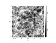
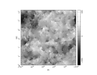
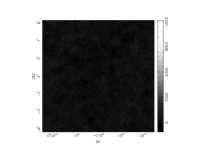
Figure 4: Three of the simulated-skies used in the simulations. Shown are the Gaussian CMB realisation (left), the pure cosmic strings map (middle) and the CMB/point sources (subtracted to 5mJy) (right).

We have detailed methods of obtaining significance levels for all of the individual statistics we are considering. However, we can place stronger limits on non-Gaussianity by combining these statistics in varying ways. We note that this will not be attempted for the Bayesian joint estimation analysis, which assumes a different PDF model in each case, and also that the CMB power spectrum is divided into different band powers, making such a combination unsuitable. We therefore only combine the map plane statistics. The combinations used are listed in the first column of Table 1.

To produce an overall significance level for a given combination, we need to calculate the value of some test function of the individual statistics included. An obvious choice would be a chi-squared test. However, many of the statistics used in this paper are drawn from non-normal distributions (see e.g. Fig. 3), making a standard chi-squared test unsuitable. A non-normal version of the chi-squared has been derived (Ferreira et al., 1998) but as noted by Barreiro & Hobson (2001) for the wavelet statistics in particular, it is very hard to evaluate. We therefore follow the method of Mukherjee et al. (2000) and use a test function that is simply the number of individual statistics in the combination that show a 95% significant deviation from Gaussianity. The combined significance level is therefore the proportion of EGRs with test function values smaller than that obtained for the real data. It is noted that this method will not identify a single highly non-Gaussian statistic value. However, any such case will be self evident, and so this does not present a problem.

4 Analysis of simulated observations

In order to characterise the effectiveness of our chosen non-Gaussianity analyses in detecting various types of non-Gaussianity, we applied them to simulated VSA observations of a number of underlying simulated-skies. The simulated observations are produced in the same way as the EGR (see above), except that the underlying Fourier modes are provided by the Fourier transform of the simulated-sky. The simulated observations have the same relative pointing centres, visibility-plane sampling and rms noise levels as the six fields (three compact array and three extended array) comprising the VSA1 mosaic. Therefore, the simulations realistically sample the visibility plane and include realistic levels of Gaussian noise.

We considered the following simulated-skies (see Fig. 4):

Gaussian CMB realisation. A Gaussian realisation of the CMB with a power spectrum given by the VSA best-fit cosmological parameters for the CDM cosmological model (see Paper VI). This is included principally to ensure that our non-Gaussianity tests do not produce spurious detections.

Pure cosmic strings. A map containing cosmic strings networks (Bouchet et al., 1988). The map is scaled to have a pixel rms equal to that of the Gaussian CMB map. It is noted that we only use a single realisation here. While it is clearly preferable to run any analysis on many different realisations, the lack of a large set of strings simulations prevents this. The analyses of this map do not therefore contain the effect of sample variance.

Composite Gaussian/strings. The sum of the above Gaussian CMB and strings maps, rescaled to have the same rms as either individual map.

Bright point sources/CMB. A power law distribution of point sources defined by the extrapolation to 34 GHz of 15 GHz source counts made by the Ryle telescope (see Paper II for details).

Source subtracted. The same point source distribution plus CMB as above, but with all sources above a given flux density removed (to mimic the VSA source subtraction strategy). Subtraction levels of 20mJy, 10mJy and 5mJy are considered. The VSA data analysed in this paper has a nominal source subtraction level of 20mJy. See Paper II for a more detailed discussion.

4.1 Visibility plane simulations

Figure 5: Example detection of the presence of bright points sources in the data using the joint estimation analysis. Shown is the marginalised posterior probability distribution calculated from simulated extended array data in an annular visibility plane band centred about $\ell=1085$. The solid and dashed lines show the results with and without the bright point sources.

Figure 6: Example test functions for simulations of various simulated-skies. The stars show the test function values for the EGR, and the vertical bars show the test function values for the simulations. Both are calculated from 1000 realisations. The rows of images show the results for pure strings (top row), composite strings (second row), 20mJy (third row), 10mJy (fourth row) and 5mJy (5th row) source subtraction levels.

We applied the Bayesian joint estimation analysis to each of the 6 field centres individually. Computing constraints mean we are unable to use Monte Carlo techniques to characterise the test fully (each analysis takes several hours). We therefore focus on unambiguous detections.

Simulated observations of the Gaussian CMB field produced no statistically significant detections. Moreover, this approach was found to be insensitive to the presence of cosmic string networks in both the composite and pure strings simulations. However, clear detections were obtained in the presence of bright point sources. The most significant detection occurred in one extended array field where three sources were present, two with fluxes of order 200  mJy, and one of order 100 mJy (see Fig. 5, solid line).

Analysis of the same simulated data where all point sources above a flux of 20 mJy (the level of subtraction applied to the real extended array data) were removed produced a marginal detection in the same extended array field.

It is noted that in the visibility plane, information about the sky (in the form of Fourier modes) has been convolved by the aperture illumination function. Any visibility is therefore a linear combination of several (possibly non-Gaussian) Fourier modes. This combination tends, because of the central limit theorem, to lessen the amount of non-Gaussianity present. We expect this effect to impair the ability of the joint estimation analysis to detect cosmological non-Gaussian structure. It is, however, ideally suited to detect non-Gaussianity in the visibility plane which, by a similar argument, would be poorly detected by map plane statistics. It is therefore important to analyse both planes.

4.2 Map plane simulations

We made 1000 simulated observations of each sky, each with a different noise realisation. By calculating individual statistics and combining them into test functions for all 1000 simulated observations, as well as for 1000 EGR, we produce distributions that show the power of any given statistic or test function to detect the presence of the simulated sky.

We applied the map plane analyses to mosaic maps of the simulated data. See Fig. 6 for examples of results of three of the tests, namely map cumulants, Minkowski functional: perimeter and the Daubechies-4 kurtosis wavelet test. We found that simulated observations of the Gaussian CMB field produced no statistically significant detections in any of our tests.

The pure cosmic strings were detected by all three tests. In particular, the Minkowski functionals and wavelet test are clearly highly sensitive to the presence of pure cosmic strings. In contrast, none of the tests were sensitive to the presence of the composite strings/Gaussian CMB simulated-sky.

All of the tests were highly sensitive to the presence of bright point sources, and were able to detect the presence of a source distribution up to 20 mJy. At 10 mJy, the wavelet test is still marginally sensitive to their presence, even though the other two tests are no longer sufficiently sensitive. At 5 mJy, all the tests are insensitive to the presence of sources.

5 Analysis of VSA observations

We applied all of our chosen non-Gaussianity tests to the VSA observations. The joint estimation test is applied separately to the data for each of the 17 individual fields. The map plane tests were applied separately to each of the 3 mosaiced fields.

5.1 Visibility plane results

For all 17 individual pointing centres, no statistically significant deviations from Gaussianity were detected.

During the early stages of the reduction of the compact array fields, this technique detected significant non-Gaussianity in the data from 3 fields. Further investigation showed that these detections were caused by a small number of high amplitude visibilities in the data (no more than 5 in each case, and as few as a single point). In all cases, they were unambiguously traced to residual spurious signal (see Paper I) and removed. Fig. 7 shows an example of the likelihood functions obtained before and after the removal of a single contaminated point.

While the basic VSA data reduction procedure has been demonstrated to deal more than adequately with the spurious signal, this technique has served as an excellent additional diagnostic of the VSA data, saving considerable time and effort during data reduction. It is now used as a standard part of the VSA data reduction process.

Figure 7: Example marginalised posterior probability distribution obtained from analysing one of the compact array fields during data reduction using the joint estimation analysis. The data were subsequently discovered to be contaminated by residual spurious signal in a single binned visibility. The annular bin analysed here contained 47 binned visibilities. The solid and dashed curves show the data with and without the contamination.

5.2 Map plane results

The combined test function values and significance levels are given in Table 1. The highest significance obtained was 96.7% , in the VSA1 mosaic, from the combined wavelet kurtosis statistics, using the Daubechies-4 basis. The highest significances in the VSA2 and VSA3 mosaics were 87.3% and 74.8%, using the area Minkowski functional and the Daubechies-4 kurtosis wavelet test, respectively. Figs. 10, 10 and 10 show example EGR test functions for the VSA1, VSA2 and VSA3 mosaics. In each case, these functions are determined from the 1000 EGR calculated for each data set. The value of the test function obtained for the real data is shown as the solid vertical line.

While the 96.7% detection in the VSA1 mosaic hints at the presence of a source of non-Gaussianity, the significance level is not high enough to rule out Gaussianity. Moreover, it is noteworthy that simulations showed the Daubechies-4 kurtosis wavelet test in particular to be sensitive to realistic point source distributions below the VSA’s source subtraction level. Therefore, this detection may be the result of slight point source contamination. Another point of note is that the VSA1 mosaic is predicted to have almost double the Galactic foreground contamination of the other two mosaics ($5.5~{}\mu K$, as opposed to $2.7~{}\mu K$ in the VSA3 mosaic; see Paper II for details). Whilst this is not a major contaminant, the Daubechies-4 kurtosis wavelet test may be sensitive enough to detect it. The addition of further extended array data to this data set will significantly improve our sensitivity to non-Gaussianity and may enable us to either identify the source of the non-Gaussianity in the VSA1 mosaic, or rule it out as a chance statistical fluctuation.

That significant non-Gaussianity detections are not found in all three mosaics confirms the success of our source surveying and subtraction strategy. Simulations show that if the power law distribution of radio sources predicted from our source surveying observations continues below 20 mJy, we would expect a detection in approximately one field in three using the Daubechies-4 kurtosis wavelet test - as indeed we find. Note that the VSA power spectrum (see Paper V) includes a statistical correction for this predicted residual point source contamination.

Figure 8: VSA1 mosaic example results and Gaussian test functions. The Gaussian test functions are denoted by stars, and the value calculated from the actual data is shown by a vertical bar.

Figure 9: VSA2 mosaic example results and Gaussian test functions

Figure 10: VSA3 mosaic example results and Gaussian test functions

Case of non-Gaussianity test	number of individual statistics	VSA1	VSA2	VSA3
cumulant	6	1 (84.0%)	0 (0%)	0 (0%)
Minkowski: area	51	1 (56.3%)	5 (87.3%)	2 (69.8%)
Minkowski: perimeter	51	1 (48.3%)	3 (76.7%)	1 (51.0%)
Minkowski: genus	51	1 (43.3%)	2 (70.7%)	2 (67.9%)
Wavelet skewness (Haar basis)	21	0 (0%)	1 (43.8%)	0 (0%)
Wavelet kurtosis (Haar basis)	21	2 (75.7%)	3 (87.4%)	1 (44.9%)
Wavelet skewness (Daubechies-4 basis)	21	0 (0%)	1 (39.4%)	0 (0%)
Wavelet kurtosis (Daubechies-4 basis)	21	4 (96.7%)	1 (41.4%)	2 (74.8%)
Wavelet skewness (Daubechies-6 basis)	21	1 (37.0%)	0 (0%)	1 (40.7%)
Wavelet kurtosis (Daubechies-6 basis)	21	1 (37.0%)	0 (0%)	0 (0%)
Wavelet skewness (Daubechies-12 basis)	21	1 (41.3%)	0 (0%)	0 (0%)
Wavelet kurtosis (Daubechies-12 basis)	21	3 (91.1%)	1 (35.7%)	2 (72.6%)
Wavelet skewness (Daubechies-20 basis)	21	2 (71.3%)	1 (40.8%)	0 (0%)
Wavelet kurtosis (Daubechies-20 basis)	21	0 (0%)	1 (37.6%)	0 (0%)
Wavelet skewness (Coiflet-2 basis)	21	1 (42.3%)	0 (0%)	1 (41.3%)
Wavelet kurtosis (Coiflet-2 basis)	21	1 (36.0%)	0 (0%)	1 (39.2%)
Wavelet skewness (Coiflet-3 basis)	21	2 (72.4%)	1 (40.4%)	1 (40.5%)
Wavelet kurtosis (Coiflet-3 basis)	21	1 (33.7%)	0 (0%)	1 (35.4%)
Wavelet skewness (Symmlet-6 basis)	21	0 (0%)	0 (0%)	0 (0%)
Wavelet kurtosis (Symmlet-6 basis)	21	1 (37.0%)	1 (37.8%)	1 (35.7%)
Wavelet skewness (Symmlet-8 basis)	21	0 (0%)	0 (0%)	0 (0%)
Wavelet kurtosis (Symmlet-8 basis)	21	2 (71.0%)	1 (36.3%)	0 (0%)
Combined Minkowski functionals	153	3 (50.8%)	10 (86.0%)	5 (68.1%)
Combined Wavelet (Haar basis)	42	2 (48.4%)	4 (80.0%)	1 (24.2%)
Combined Wavelet (Daubechies-4 basis)	42	4 (80.7%)	2 (44.8%)	2 (45.4%)
Combined Wavelet (Daubechies-6 basis)	42	2 (45.8%)	0 (0%)	1 (19.8%)
Combined Wavelet (Daubechies-12 basis)	42	4 (82.3%)	1 (18.2%)	2 (45.7%)
Combined Wavelet (Daubechies-20 basis)	42	2 (43.1%)	2 (45.3%)	0 (0%)
Combined Wavelet (Coiflet-2 basis)	42	2 (45.4%)	0 (0%)	2 (45.5%)
Combined Wavelet (Coiflet-3 basis)	42	3 (67.1%)	1 (18.5%)	2 (44.3%)
Combined Wavelet (Symmlet-6 basis)	42	1 (18.2%)	1 (19.0%)	1 (20.0%)
Combined Wavelet (Symmlet-8 basis)	42	2 (43.8%)	1 (19.6%)	0 (0%)

Table 1: Test function values and combined significance levels for the different cases of each map plane non-Gaussianity test. The results for each of the three VSA mosaics are given.

6 Conclusions

We have analysed the VSA data sets presented in Papers V and VI for the presence of non-Gaussianity. We have found the following:

• The VSA2 and VSA3 mosaics are consistent with Gaussianity.

• In the VSA1 mosaic, a 96.7% detection of non-Gaussianity was found with the kurtosis wavelet test (using the Daubechies-4 wavelet basis). We conclude that while this may hint at a source of non-Gaussianity, the level is consistent with that expected for the known residual point source contamination in the VSA data. It is therefore unlikely to be cosmological in origin.

• Non-Gaussianity testing in the visibility plane has proven an invaluable tool for locating systematic effects in data. It is therefore vitally important to test interferometric observations of the CMB for non-Gaussianity in both the visibility and map planes.

References

- Aghanim et al. (2003) Aghanim N., Kunz M., Castro P. G., Forno O., 2003, Non-Gaussianity: Comparing wavelet and Fourier based methods, submitted to Astronomy and Astrophysics; astro-ph/0301220
- Banday et al. (2000) Banday A. J., Zaroubi S., Górski K. M., 2000, ApJ, 533, 575
- Barreiro & Hobson (2001) Barreiro R. B., Hobson M. P., 2001, MNRAS, 327, 813
- Bartolo & Liddle (2002) Bartolo N., Liddle A. R., 2002, Phys.Rev.D, 65, 121301
- Bond et al. (1998) Bond J. R., Jaffe A. H., Knox L., 1998, Phys.Rev.D, 57, 2117
- Bouchet et al. (1988) Bouchet F. R., Bennett D. P., Stebbins A., 1988, Nature, 335, 410
- Chiang et al. (2003) Chiang L., Naselsky P. D., Verkhodanov O. V., Way M. J., 2003, ApJ, 590, L65
- Chiang et al. (2002) Chiang L. Y., Naselsky P., Coles P., 2002, Phase Mapping as a Powerful Diagnostic of Primordial Non-Gaussianity, astro-ph/0208235
- Contaldi et al. (1999) Contaldi C., Bean R., Magueijo J., 1999, Phys.Rev.B, 468, 189
- Ferreira et al. (1998) Ferreira P. G., Magueijo J., Gorski K. M., 1998, ApJ, 503, L1+
- Ferreira et al. (1997) Ferreira P. G., Magueijo J., Silk J., 1997, Phys.Rev.D, 56, 4592
- Grainge et al. (2003) Grainge K., et al., 2003, MNRAS, 341, L23
- Hansen et al. (2002) Hansen F. K., Marinucci D., Natoli P., Vittorio N., 2002, Phys.Rev.D, 66, 63006
- Hobson et al. (1999) Hobson M. P., Jones A. W., Lasenby A. N., 1999, MNRAS, 309, 125
- Hobson & Maisinger (2002) Hobson M. P., Maisinger K., 2002, MNRAS, 334, 569
- Komatsu et al. (2003) Komatsu E., et al., 2003, First Year Wilkinson Microwave Anisotropy Probe (WMAP) Observations: Tests of Gaussianity, submitted to ApJ; astro-ph/0302223
- Maisinger et al. (1997) Maisinger K., Hobson M. P., Lasenby A. N., 1997, MNRAS, 290, 313
- Maisinger et al. (1998) Maisinger K., Hobson M. P., Lasenby A. N., Turok N., 1998, MNRAS, 297, 531
- Mukherjee et al. (2000) Mukherjee P., Hobson M. P., Lasenby A. N., 2000, MNRAS, 318, 1157
- Peebles (1999) Peebles P. J. E., 1999, ApJ, 510, 531
- Polenta et al. (2002) Polenta G., et al., 2002, ApJ, 572, L27
- Rocha et al. (2001) Rocha G., Magueijo J., Hobson M., Lasenby A., 2001, Phys.Rev.D, 64, 63512
- Rubiño-Martin et al. (2003) Rubiño-Martin J. A., et al., 2003, MNRAS, 341, 1084
- Santos et al. (2003) Santos M. G., Heavens A., Balbi A., Borrill J., Ferreira P. G., Hanany S., Jaffe A. H., Lee A. T., Rabii B., Richards P. L., Smoot G. F., Stompor R., Winant C. D., Wu J. H. P., 2003, MNRAS, 341, 623
- Scott et al. (2003) Scott P. F., et al., 2003, MNRAS, 341, 1076
- Slosar et al. (2003) Slosar A., et al., 2003, MNRAS, 341, L29
- Taylor et al. (2003) Taylor A. C., et al., 2003, MNRAS, 341, 1066
- Troia et al. (2003) Troia G. D., et al., 2003, The trispectrum of the Cosmic Microwave Background on sub-degree angular scales: an analysis of the BOOMERanG data, submitted to MNRAS; astro-ph/0301294
- Verde & Heavens (2001) Verde L., Heavens A. F., 2001, ApJ, 553, 14
- Waldram et al. (2003) Waldram E. M., Pooley G. G., Grainge K. J. B., Jones M. E., Saunders R. D. E., Scott P. F., Taylor A. C., 2003, MNRAS, 342, 915
- Wang & Kamionkowski (2000) Wang L., Kamionkowski M., 2000, Phys.Rev.D, 61, 63504
- Watson et al. (2003) Watson R. A., et al., 2003, MNRAS, 341, 1057
- Wu et al. (2001) Wu J. H., Balbi A., Borrill J., Ferreira P. G., Hanany S., Jaffe A. H., Lee A. T., Rabii B., Richards P. L., Smoot G. F., Stompor R., Winant C. D., 2001, Physical Review Letters, 87, 251303