High Precision Differential Astrometry

Abstract

While conventional imaging in VLBI provides information only about the relative position between different features of a given source, phase-referenced observations can provide precise positional information with respect to an external reference. The use of differential techniques relies on the fact that most of the instrumental and propagation effects are common for radio sources sufficiently close together in the sky. These effects cancel by subtracting the visibility phases of the reference source from that of the neighboring objects. Differential VLBI astrometry yields relative positions of radio sources with sub-milliarcsecond accuracy. These high precisions can be applied to solve various astrophysical problems. In this paper I will review the progress made recently in this field, both in technique and science.

Max-Planck-Institut für Radioastronomie, Bonn, Germany

1. The technique

Astrometry is the domain of astronomy devoted to the determination of positions and their time-variations. In the radio domain, sub-milliarcsecond accuracy is reached through high-precision very-long-baseline interferometry (VLBI), using the positional information obtained from the fringe phases.

The theoretical positional precision of an interferometer is $\sigma_{\rm R.A.,\,Dec}=(1/2\pi)\times(1/{\rm SNR})\times(\lambda/D)$, where SNR is the signal-to-noise ratio, $\lambda$ is the wavelength, and $D$ is the baseline length (Lestrade et al. 1990). For SNR$\sim$15, $D=8000$ km, and $\lambda$=3.6 cm, a precision of 10 $\mu$as is possible; $\lambda$ 1.3 cm yields 4 $\mu$as, and $\lambda$ 0.7 cm, 2 $\mu$as. Comparable precisions will be obtained by the optical, astrometric satellites, such as the Space Interferometric Mission (SIM), with 4 $\mu$as in pointed mode, or GAIA, with 1 (10) $\mu$as for magnitudes of 5 (10) in survey mode. The Atacama Large Millimetre Array (ALMA) will have $D=10$ km, and for a SNR$\sim$15 and $\lambda$ 0.87 mm, a precision of 200 $\mu$as will be obtained, much poorer than VLBI values.

The main astrometric observable is the delay, directly related to the fringe phase as a function of frequency. It can be described as $\tau_{\rm geom}=\vec{D}\cdot\hat{s}/c$, where $\vec{D}$ is the baseline vector and $\hat{s}$ a unit vector towards the observed source. It is directly related to the total phase $\phi_{\rm T}$ from the interferometer output (visibility function with amplitude and phase, $A\cos\phi_{\rm T}$, $\phi_{\rm T}\sim 2\pi\nu\tau$).

To determine relative positions in the sky, two neighboring sources are observed and their relative phases are determined, either simultaneously if they are both within the primary antenna beam of each element of the interferometer, or alternately if switching from one source to the other is needed. The observation of neighboring sources cancels out most of the systematic effects in the astrometric data reduction, since they are mostly common for both. We analyze the observable of one source subtracted from the other, that is, we perform differential astrometry. Most of the geometrical parameters involved in the observation are taken account of and removed during the correlation process, leaving one to work with the residuals.

The relevant residual quantities measured are the phase delay as $\tau_{\phi}=(\phi_{\rm T}+2\pi n)/(2\pi\nu)$, where $n$ is an unknown integer; the group delay which gives the change of phase with frequency, $\tau_{\rm G}=(1/2\pi)\times(\partial\phi_{\rm T}/\partial\nu)$; and the delay rate, which measures the change of delay with time, as $\dot{\tau}=(1/2\pi\nu)\times(\partial\phi_{\rm T}/\partial t)$. The group delay and the delay rate are unambiguous observables, but less precise than the phase-delay, which is $n/\nu$-ambiguous.

1.1. Phase-reference mapping vs. phase-delay astrometry

The residual, differential phase can be split in the following terms:

$$\begin{array}[]{ccccccccc}\phi_{{\rm A}-{\rm B}}^{\rm res}&=&\phi_{{\rm A}-{\rm B}}^{\rm res,\,\sl str}&+&\phi_{{\rm A}-{\rm B}}^{\rm res,\,\sl pos}&+&\phi_{{\rm A}-{\rm B}}^{\rm res,\,\sl inst}&+&\phi_{{\rm A}-{\rm B}}^{\rm res,\,\sl prop}\,,\\[4.0pt] &&\scriptsize{(1)}&&\scriptsize{(2)}&&\scriptsize{(3)}&&\scriptsize{(4)}\\ \end{array}$$

namely, the structural term (caused by the fact that radio sources are not point-like), the positional term, the instrumental term (antenna electronics, clocks, etc.), and the unmodeled term of the propagation medium (atmosphere, ionosphere).

Phase-delay astrometry.

Assuming both sources are strong enough to be detected, if we provide an a priori model for (3) & (4), and we remove (1) by using hybrid maps from the two sources, we determine (2) (and corrections for (3) and (4)) via a weighted least-squares fit. This process also needs to solve for the phase ambiguities, which is known as phase-connection (Shapiro et al. 1979). Historically, this was the first approach to perform high precision differential astrometry.

Phase-reference mapping.

Assuming that the residuals (3) and (4) are sufficiently small, the phase from one source (the strong one) is interpolated to the other one and a Fourier-transform is performed:

$$|V(u,v)|e^{i\phi_{{\rm A}-{\rm B}}}\longrightarrow I(x,y)=\int\int V(u,v)e^{-i2\pi(ux+vy)}\,du\,dv\,,$$

where $(x,y)$ are the coordinates in the image plane, and $(u,v)$ their Fourier-pairs, $V$ is the visibility function, and $I$ is the brightness distribution. By this process an image with some offset position from the origin is obtained, recovering also the structure of the source. The first phase-reference map with in-beam observations (1038+528 A/B, 33^′′ separation) was published by Marcaide & Shapiro (1984). The first one from switched observations (0249+436/0248+483, 0$\hbox to0.0pt{.\hss}^{\circ}$5 sep.) was presented in Alef (1988).

A method related to the phase-reference mapping is the hybrid double mapping (see Rioja & Porcas 2000), where the visibility functions of two nearby sources are added together and both are imaged in the same field; therefore, the offset in one of the images w.r.t. the other in the map is the difference between their a priori coordinate differences and the ‘true’ value. The fast-frequency switching presented by Middelberg et al. (2002) interpolates the phase from one frequency to another frequency by multiplying by the frequency ratio.

The cluster-cluster (or multi-view) method, first presented by Counselman et al. (1974), uses a common local oscillator for multiple antenna elements (a “cluster”) in different sites. This enables simultaneous observations of multiple sources to be made on the separate “sub-baselines” between sub-elements from one site to another. Recently, Rioja et al. (2002) reported on successful observations at 1.6 GHz.

1.2. Recent technical achievements

In recent years, some progress has allowed highest astrometric precisions to be obtained, reaching higher frequencies, etc. One key aspect is the removal of the delay term introduced by the ionospheric plasma, which is frequency-dependent. Classical geodetic experiments use dual-band observations (2.3/8.4 GHz) to account for this. The development of the Global Positioning System (GPS) in the 1990s made it possible to estimate the total electron content (TEC) between a GPS receiver site and a dual-frequency transmitting satellite. Using measurements made at sites near to VLBI sites, it is possible to estimate the ionospheric contribution to the VLBI observables. This was shown by Ros et al. (2000), and now the ionospheric correction can be performed routinely from global IONEX TEC data within $\cal A$$\cal I$$\cal P$$\cal S$ using the task tecor (see, e.g., Walker & Chatterjee 1999).

In phase-delay astrometry, phase-connection has been extended up to distances of 15^∘ (Pérez-Torres et al. 2000), and up to frequencies of 43 GHz (Guirado et al. 2000). A phase-referencing test at 86 GHz has also been successful (Porcas & Rioja 2002). Fomalont & Kopeikin (2002) and Fomalont et al. (these proceedings) have shown that, using multiple calibrators at 8.4 GHz, precisions below 10 $\mu$as can be obtained by phase-referencing.

The application of astrometry to orbiting VLBI has been limited by the fact that the satellite HALCA could not observe in nodding mode. In-beam observations at 5 GHz have been successful (Porcas et al. 2000; Guirado et al. 2001), yielding an upper bound of 10 m to the uncertainty of the spacecraft orbit reconstruction.

2. The Science

The relative angular positions of extragalactic radio sources inferred from VLBI astrometry form the best realization of an inertial reference frame in astronomy. A continuous program of monitoring hundreds of radio sources establishes and maintains two reference frames: the terrestrial (antenna positions with mm-accuracy) and the celestial (see, e.g., Sovers et al. 1998). The International Astronomical Union adopted the International Celestial Reference Frame (ICRF) as the fundamental one (see Ma et al. 1997, 1998). The ICRF improves the precision of the latest optical “fundamental catalogue”, the FK5 (Fricke et al. 1988) by more than one order of magnitude. Special techniques must be used to connect the VLBI celestial frame to the historical optical frame (Lestrade et al. 1995). This is of special importance with the optical satellites like HIPPARCOS, SIM, or GAIA, which have a precision equal to, or better than VLBI.

The accurate determination of positions of celestial bodies has many applications in radio astronomy. Astrometry of stellar masers is covered in the review given by Boboltz (these proceedings). High-precision astrometry has been applied to determine the positions, proper motions, and parallaxes of pulsars (see, e.g., Campbell et al. 1996 and Brisken, these proceedings). The registration of the young supernova remnant SN 1993J w.r.t. the nucleus of M 81 (Bietenholz et al. 2001) gave the position of the dynamical center of the shell emission and limited any possible one-sided expansion of the shell to 5.5%. VLBI astrometry has also been applied to determine the Galactic Center position w.r.t. J1745$-$285 and J1748$-$291 at 43 GHz, yielding an estimate of its proper motion and a lower limit to its mass (see Reid et al., these proceedings).

The astrometric technique also allows some of the predictions of general relativity to be tested, by analyzing the effect on the incoming signals by their passage through the varying gravitational potential within the Solar System. Lebach et al. (1995) determined the value $\gamma_{\rm PPN}=0.9996\pm 0.0017$ for the parameterized post-Newtonian relativity theory, from group-delay observations of 3C 279 w.r.t. 3C 273 during a solar occultation. Recently, the speed of gravity has been measured during the September 2002 Jupiter conjunction with the QSO J0832+1835, providing the parameter $\delta=(c/c_{\rm grav})-1=-0.02\pm 0.19$ that yields a value of $c_{\rm grav}=1.06\pm 0.21c$ (Fomalont & Kopeikin 2003). The detection of the frame dragging of the terrestrial gravitational potential (expected to be 42 mas yr^-1) is the purpose of the Gravity Probe B mission, where IM Pegasi (HR 8703) will be used as a guide star. Astrometric observations have been carried out on this flaring star since 1997 to fix its astrometric parameters within 150 $\mu$as yr^-1 (see Lebach et al. 1999 and Ransom et al., these proceedings). Honma & Kurayama (2002) suggest that VLBI astrometry could even be used to study gravitational micro-lensing.

AGN studies.

Following the standard jet model in active galactic nuclei (AGN), the opacity $\sim 1$ surface (a.k.a. the core) has a frequency-dependent position. The registration of close pairs of AGN allows the stability of the core in time and its changes with frequency to be determined. For instance, Bartel et al. (1986) showed that the core in 3C 345 is stable within 20 $\mu$as yr^-1. Marcaide & Shapiro (1984) proved that the core position in the QSO 1038+528 A is frequency-dependent, by determining its position w.r.t. 1038+528 B via in-beam observations. The upper limit on the proper motion of one core w.r.t. to the other is 10 $\mu$as yr^-1 (Rioja & Porcas 2000). Guirado et al. (1995) determined the position of 4C 39.25 w.r.t. the reference source 0920+390 and could establish a proper motion of its B component of $90\pm 43$ $\mu$as yr^-1 in R.A. and $7\pm 68$ $\mu$as yr^-1 in Dec., confirming the nature of this component as a shock wave. This result was later confirmed by the geodetic data presented in Fey et al. (1997). Ros et al. (1999) compared the estimated position of 1928+738 w.r.t. 2007+777 from epochs 1985 to 1992, and observed changes in the position of the VLBI core. This implies that the dynamical center of this QSO is to the north of the core.

These observations, together with the extension of the phase connection technique to distances of 15^∘ (Pérez-Torres et al. 2001), has lead to a project of observations to establish the absolute kinematics of radio source components in the thirteen radio sources of the S5 polar cap sample (first images are presented in Ros et al. 2001), which is being carried out at frequencies of 8.4, 15, and 43 GHz. These phase-delay observations use bootstrapping techniques and the geometrical constraints given by the location of all the radio sources within 30^∘ of the north celestial pole.

Stellar astrometry — search for exo-planets.

We have mentioned above the importance of the link between the reference frame provided by HIPPARCOS and VLBI measurements. This has been done by Lestrade et al. (1995, 1999) using 11 radio stars in the northern and southern hemispheres. One of the stars initially chosen for this work was the flaring AB Doradus, which exhibited large residuals after solving for proper motion and parallax. Guirado et al. (1997) presented a detailed analysis combining HIPPARCOS and VLBI solutions, showing the presence of a low mass companion of 0.08$-$0.11 M_⊙ orbiting the catalogue star (of 0.76 M_⊙). This experiment demonstrates the feasibility of detecting brown dwarfs and exo-planets orbiting stars at tens of parsecs.

The radial velocity method (based on Doppler shift measurements) of detecting exo-planets favors the detection of objects at short orbital radii and large speeds. In contrast, astrometric measurements of the “wobble” favor the detection of planets at large orbital radii (which need longer observing campaigns, since the orbital periods can be tens of years). In Fig. 1 we show in detail the region accesible to VLBI astrometry. A program of this kind is being carried out using the small but sensitive array consisting of the DSN antennas and Effelsberg, observing nearby M dwarfs with a resolution of 1 mas (first results are shown in Guirado et al. 2002).

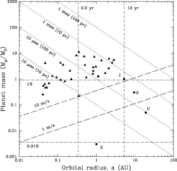
Figure 1.: Detection domains for methods aimed at detecting exo-planet orbital motion, assuming M_⋆ = M_⊙. Triangles design lower limits on the masses of known planetary systems, and circles denote Jupiter (J), Saturn (S), Uranus (U), and the Earth (E). The diagonal lines show the exo-planet detection limits for radial velocity and wobble measurements. Horizontal lines show photometric detection thresholds for planetary transits of 1% and 0.01%, corresponding roughly to Jupiter and the Earth. The region below 10 m s^-1 and above 10 $\mu$as (at 10 pc) is ‘reserved’ for exploration in astrometry. Figure taken from Perryman, Rep. Prog. Phys., 63, (2000).

3. The Future

The construction of the VLBA facilitated astrometric observations in the last decade, thanks to the high slewing speeds of the antennas for nodding between sources, and the automization of the data reduction. Together with the advent of the SIM and GAIA era, high resolution radio astrometry will also experience progress during the coming years. Improvement of the geometrical models will play a role (better determination of polar motion, the mapping functions which describe the behavior of the atmospheric delay as a function of elevation, antenna positions, etc.). Progress is being made in modeling the propagation medium, using water vapor radiometers and improved GPS analyses. A more timely correlation (e.g., by eVLBI, see Garrington, these proceedings) will facilitate more rapid results for of the length of the day and other geodetic/astrometric parameters. The implementation of nodding capabilities in future space VLBI missions would also enhance the astrometric precision for sources separated by a few degrees, given the higher resolution provided by baselines longer than the Earth size (assuming that the spacecraft orbit parameters are well-determined). The continuous improvement in antenna performance and new elements being added to the VLBI networks will provide more and better data. Finally, a new arrays designed for astrometry is underway, the VERA project (Kobayashi, these proceedings). For the planned Square Kilometer Array (SKA) telescope, a set of interesting suggestions for high-resolution options for astrometry has been proposed by Charlot (2001).

Acknowledgments.

I am grateful to R. W. Porcas, J. C. Guirado, W. Alef, and M. Kadler for their careful reading and helpful comments on this manuscript.

References

Alef, W. 1988, in IAU Symp. 129, The Impact of VLBI on Astrophysics and Geophysics, ed. M. J. Reid & J. M. Moran (Dordrecht: Kluwer), 523

Bartel, N., et al. 1986, Nature, 319, 733

Bietenholz, M. F., Bartel, N., & Rupen, M. P. 2001, ApJ, 557, 770

Campbell, R. M., et al. 1996, ApJ, 461, L95

Charlot, P. 2001, Astrometry with the SKA, in High Resolution Options for the SKA, Bonn, 10-11 December 2001, http://www.euska.org/workshops/hr_ws_MPIfR_Bonn.html

Counselman, C. C., et al. 1974, Phys.Rev.Lett, 33, 1621

Fey, A. L., Eubanks, M., & Kingham, K. A. 1997, AJ, 114, 2284

Fricke, W., et al. 1988, Fifth fundamental catalogue (FK5). Part 1: The basic fundamental stars, (Heidelberg: Astronomische Rechen-Inst.)

Fomalont, E. B., & Kopeikin, S. 2002, in Proc. of the 6th EVN Symp., ed. E. Ros et al., (Bonn: MPIfR), 53

Fomalont, E. B., & Kopeikin, S. 2003, astro-ph/0302294

Guirado, J. C., et al. 1995, AJ, 110, 2586

Guirado, J. C., et al. 1997, ApJ, 490, 835

Guirado, J. C., et al. 2000, A&A, 353, L37

Guirado, J. C., et al. 2001, A&A, 371, 766

Guirado, J. C., et al. 2002, in Proc. of the 6th EVN Symp., ed. E. Ros et al., (Bonn: MPIfR), 255

Honma, M., & Kurayama, T. 2002, ApJ, 568, 717

Lebach, D. E., et al. 1995, Phys.Rev.Lett, 75(8), 1439

Lebach, D. E., et al. 1999, ApJ, 517, L43

Lestrade, J.-F., et al. 1990, AJ, 99, 1663

Lestrade, J.-F., et al. 1995, A&A, 304, 182

Lestrade, J.-F., et al. 1999, A&A, 344, 1014

Ma, C., et al. 1997, in IERS Technical Note 23, ed. C. Ma & M. Feissel (Paris: Observatoire de Paris)

Ma, C., et al. 1998, AJ, 116, 516

Marcaide, J. M., & Shapiro, I. I. 1984, ApJ, 276, 56

Middelberg, E., et al. 2002, in Proc. of the 6th EVN Symp., ed. E. Ros et al., (Bonn: MPIfR), 61

Pérez-Torres, M. A., et al. 2000, A&A, 360, 161

Perryman, M. A. C. 2000, Rep. Prog. Phys., 63, 1209

Porcas, R. W., et al. 2000, in Astrophysical Phenomena Revealed by Space VLBI, ed. H. Hirabayashi, P. G. Edwards, & D. W. Murphy, (Tokyo: ISAS), 245

Porcas, R. W., & Rioja, M. J. 2002, in Proc. of the 6th EVN Symp., ed. E. Ros et al., (Bonn: MPIfR), 65

Rioja, M. J., & Porcas, R. W. 2000, A&A, 355, 552

Rioja, M. J., et al. 2002, in Proc. of the 6th EVN Symp., ed. E. Ros et al., (Bonn: MPIfR), 57

Ros, E., et al. 1999, A&A, 348, 381

Ros, E., et al. 2000, A&A, 356, 357

Ros, E., et al. 2001, A&A, 376, 1090

Shapiro, I. I., et al. 1979, AJ, 84, 1459

Sovers, O. J., Fanselow, J. L., & Jacobs, C. S. 1998, Rev. Mod. Phys., 70, 1393

Walker, C., & Chaterjee, S., 1999, Ionospheric Corrections using GPS Based Models, VLBA Scientific Memo 23, (Socorro, NM: NRAO)