Stellar Pollution and [Fe/H] in the Hyades

Abstract

The Hyades open cluster presents a unique laboratory for planet formation and stellar pollution studies because all of the stars have essentially the same age and were born from the same cloud of gas. Furthermore, with an age of $\sim$650 Myr most of the intermediate and low mass stars are on the main sequence. Given these assumptions, the accretion of metal rich material onto the surface of a star during and shortly after the formation of planetary systems should be evident via the enhanced metallicity of the star. Building on previous work, stellar evolution models which include the effects of stellar pollution are applied to the Hyades. The results of several Monte Carlo simulations, in which the amount of accreted material is drawn at random from a Gaussian distribution with standard deviation equal to half the mean, are presented. An effective temperature–[Fe/H] relation is produced and compared to recent observations. The theoretical predictions presented in this letter will be useful in future searches for evidence of stellar pollution due to planet formation. It is concluded that stellar pollution effects at the mean level of $\geq$2 $\mathrm{M_{\oplus}}$ of iron are ruled out by the current observational data (Paulson et al., 2003).

1 Introduction

The concept of stellar pollution, that as the protoplantery disk around a star forms planets and settles into a stable configuration the star may accrete some of the metal rich material from the disk, has potentially observable implications for the parent star. The magnitude of the observable implications can vary widely, being influenced by the planetary formation process, which depends on the composition and dynamics of the cloud from which the star is born, as well as the depth of the surface mixed layer of the star, which in turn depends on the mass of the star. Murray et al. (2001) compared a sample of $\sim$500 main sequence stars in the Solar neighborhood to stellar evolution models. Their analysis showed that the observations are consistent with the stars having accreted 0.5 $\mathrm{M_{\oplus}}$ of iron on average. The sample consisted of field stars and thus the signal for pollution had to be disentangled from variations in age and bulk metallicity.

Based on the proposal by Quillen (2002) that scatter about the main sequence in the Hyades color-magnitude diagram (CMD) of de Bruijne et al. (2001) can be used to limit the level of pollution, Dotter & Chaboyer (2003, hereafter DC) applied stellar evolution models which incorporate the effects of stellar pollution to the Hyades. The authors found that pollution on the level of $\sim$1.5 $\mathrm{M_{\oplus}}$ could be ruled out by scatter in the CMD. A more direct test of pollution in the Hyades, presented in this letter, involves comparing polluted stellar evolution models to observations of [Fe/H] in Hyades stars. Such a test is possible with the high precision [Fe/H] data set presented by Paulson et al. (2003, hereafter PSC). At present, at least three other groups are known to be at work on similar observations in the Hyades (Boesgaard et al., 2002; Fulbright, 2002; Primas, et al., 2003). These observations may have the precision and wide effective temperature range to make a definitive statement about stellar pollution in the Hyades. The work of PSC is, within the quoted uncertainties, consistent with zero dispersion about the mean [Fe/H] of the sample. However, as shown below, it is also in good agreement with the predictions drawn from polluted stellar evolution models.

2 Monte Carlo Simulations

Four distinct Monte Carlo simulations were performed using Chaboyer’s stellar evolution program with modifications to deal with stellar pollution. Each simulation uses the same set of 77 stellar models described by DC. These stars lie in the effective temperature range of 3500 K to 8000 K which corresponds to masses in the range of roughly 0.5 to 2 $\mathrm{M_{\odot}}$. Each Monte Carlo simulation consists of 1000 individual runs through the set of polluted stellar models. For each stellar model in a given run, the amount of polluting material is drawn at random from a Gaussian distribution with standard deviation equal to half the mean. Murray et al. (2001) find that, on average, field stars in the Solar neighborhood have accreted $\sim$0.5 $\mathrm{M_{\oplus}}$ of iron. Three of the four simulations have means of 0.5, 1, and 2 $\mathrm{M_{\oplus}}$ of iron. The fourth simulation begins with a mean of 0.5 $\mathrm{M_{\oplus}}$ but adds in a 5% probability that a star will have giant planet in a tight orbit leading to an average accretion of 5 $\mathrm{M_{\oplus}}$ of iron (Murray & Chaboyer, 2002). In order that the simulations have the mean [Fe/H] = 0.13 (within a few hundredths of a dex) in agreement with observations (Boesgaard & Friel, 1990, PSC) the models have the same initial bulk metallicity, Z=0.024. The only exception is the 2 $\mathrm{M_{\oplus}}$ case for which all models have a lower initial bulk metallicity (Z=0.020) in order to keep the mean [Fe/H] reasonably close to the observed value.

The main goal of the simulations is to determine how [Fe/H] varies with stellar mass and pollution. To obtain the mass–[Fe/H] relation from one simulation, the mass–[Fe/H] relation is created for each of the individual runs. A smooth curve is fit to each individual relation using the LOWESS (Locally Weighted Regression) technique (Cleveland, 1979). Finally, all of the 1000 individual mass–[Fe/H] curves are averaged. The process is analogous to the CMD analysis of DC. Color tables from Buser & Kurucz (1992) are used for the color transformations.

To compute overall [Fe/H] statistics for each of the four simulations, the mean [Fe/H] value is computed from the 77 stellar models in each individual run. The overall mean is the average of all 1000 individual means. The [Fe/H] statistics from each simulation are also divided into four mass bins. Within each bin the mean and standard deviation about the mean are determined from all of the stellar models which have masses in the given range.

3 Results

Table 1: Monte Carlo Results

			$\Delta$[Fe/H]
			$M_{*}<$0.6 $\mathrm{M_{\odot}}$	0.6–1.0 $\mathrm{M_{\odot}}$	1.0–1.4 $\mathrm{M_{\odot}}$	1.4–1.8 $\mathrm{M_{\odot}}$
			$\mathrm{T_{eff}}<$4000 K	4000–5400 K	5400–6500 K	6500–8000 K
No.	Accreted Mass ($\mathrm{M_{\oplus}}$ Iron)	Initial Z	B–V$>$1.35	0.74–1.35	0.43–0.74	0.23–0.43
1	0.50$\pm$0.25	0.024	0.000$\pm$0.002	0.001$\pm$0.004	0.017$\pm$0.019	0.086$\pm$0.079
2	#1 (95%), 5.00$\pm$2.50 (5%)	0.024	0.000$\pm$0.012	0.002$\pm$0.018	0.026$\pm$0.060	0.107$\pm$0.152
3	1.00$\pm$0.50	0.024	0.000$\pm$0.005	0.004$\pm$0.008	0.040$\pm$0.036	0.157$\pm$0.137
4	2.00$\pm$1.00	0.020	0.000$\pm$0.012	0.012$\pm$0.022	0.095$\pm$0.079	0.312$\pm$0.248

The primary results of this paper are presented in Table 1, which presents theoretical predictions for the mean [Fe/H] and its dispersion as a function of stellar mass. These predictions are presented as relative abundances rather than absolute because relative abundances are immediately obtained from observational data whereas absolute abundances introduce another source of uncertainty, namely the Solar abundances. For this reason, among others, one study may have a different mean value of [Fe/H] than another. For the purposes of testing for the existence of stellar pollution, it is the behavior of the relative abundances that matters most. At each location in the $\Delta$[Fe/H] portion of Table 1 the first value is the mean [Fe/H] value for that range of models relative to the mean for the low mass models. The second value (following the “$\pm$”) is the standard deviation about the mean as described at the end of $\S$2. In a given row, the mean value represents the difference between one mass range and another, and the standard deviation of the mean gives an idea of the dispersion within one mass range. Overall absolute abundances for the four simulations listed in Table 1 are: $<$[Fe/H]$>$=0.131$\pm$0.052 (1), 0.142$\pm$0.085 (2), 0.161$\pm$0.092 (3), and 0.155$\pm$0.176 (4).

These predictions reflect the differences in [Fe/H] exhibited by the four cases outlined in the previous section and differences within each case as a function of stellar mass. It is evident that assuming 5% of the Hyades stars have giant planets in tight orbits (case 2) increases $<$[Fe/H]$>$ by only 0.011 (8% relative change) but increases the standard deviation about the mean by 0.033 (63%) over the entire mass range covered in the simulations. Thus a small probability of having a giant planet in a tight orbit will have relatively little influence on the average metallicity of a stellar population but will have a significant influence on the scatter. The [Fe/H] data is broken into mass bins in order simplify comparisons with observational data. The Monte Carlo simulations indicate that, if stellar pollution is the main factor in metallicity variations, then stars above roughly 6500 K (1.4 $\mathrm{M_{\odot}}$) will have a significantly higher mean [Fe/H] and dispersion than stars below 6500 K. The lower the initial bulk metallicity the more pronounced this effect will be.

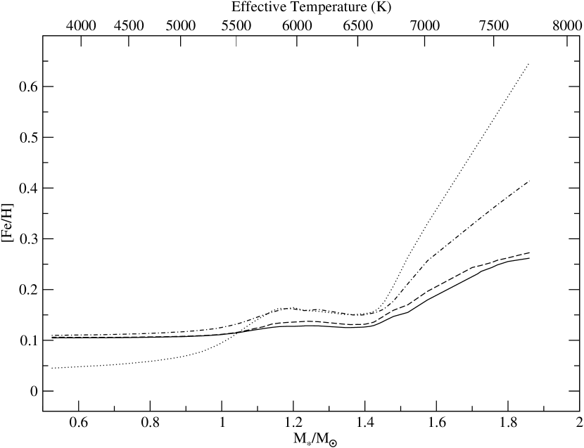
Figure 1: The mass/$\mathrm{T}_{\mathrm{eff}}$–[Fe/H] relation for the Hyades. The solid line is the 0.5 $\mathrm{M_{\oplus}}$ case (1 in Table 1), the dashed line is the 0.5 $\mathrm{M_{\oplus}}$ with giant planets case (2), the dash-dotted line is the 1.0 $\mathrm{M_{\oplus}}$ case (3), and the dotted line is the 2.0 $\mathrm{M_{\oplus}}$ case (4).

The mean mass–[Fe/H] relation is displayed for all four simulations in Figure 1. The general trend is that [Fe/H] increases with stellar mass which is consistent with the decreasing mass of the surface mixed layer. The decrease at around 1.4 $\mathrm{M_{\odot}}$ is due to an artificially increased surface mixed layer, for details see Murray et al. (2001).

4 Comparison with Observational Data

The hotter temperatures and higher rotational velocities of A and F stars make the task of measuring metal abundances exceedingly difficult. As such, a detailed comparison of observations of A and F stars to the Monte Carlo simulations is not currently possible. However, comments are made regarding two studies of F and A stars in the Hyades. Boesgaard & Friel (1990) list effective temperatures and [Fe/H] values for 14 F stars in the Hyades. The uncertainties in [Fe/H] are all of order 0.10 dex and the authors find no [Fe/H] trend with temperature. Nevertheless, a simple comparison suggests that, within the uncertainties, the polluted models are in agreement with their data.

Varenne & Monier (1999) present a study of 29 F and 19 A stars in the Hyades. The authors provide uncertainties in their [Fe/H] values for only about 10 of the 48 stars, thus an analysis of the dispersion is not possible. Furthermore, the data varies widely over a range of $\sim$0.6 dex in [Fe/H] so simple averages in several temperature ranges like those in Table 1 would favor the outlying points. To avoid giving equal weight to the outliers in the average values, the averages are taken from the LOWESS fit to the data. (LOWESS weights each point based on how close it is to the local average.) In keeping with the type of analysis performed by DC and in the following paragraphs, the absolute values of the relative [Fe/H] values (relative meaning the overall average has been subtracted off) are used. The absolute value of the $\Delta$[Fe/H] data of Varenne & Monier (1999) has a LOWESS-average value of 0.05 dex between 6000 and 6500 K, and 0.12 dex between 6500 and 8000 K. Comparing these data to Table 1, LOWESS-average values in between 6000 and 6500 K are 0.04 dex (1), 0.06 dex (2), and 0.10 dex (3). Between 6500 and 8000 K the simulations have LOWESS-average values of 0.06 dex (1), 0.07 dex (2), and 0.17 dex (3). At the 90% confidence level, the Varenne & Monier (1999) data is consistent with stellar pollution at and below the 1 $\mathrm{M_{\oplus}}$ level but is inconsistent with pollution at the 2 $\mathrm{M_{\oplus}}$ level.

PSC perform spectroscopic abundance analyses of 55 Hyades stars which range in effective temperature from about 5000 to 6500 K. These authors list relative [Fe/H] data and perform detailed error analysis making it possible to directly compare the data to the predictions of the polluted stellar models. The star chosen as the standard about which the relative abundances are determined (HD 35768) has an [Fe/H] value somewhat below the cluster average so that the $\Delta$[Fe/H] values average to $\sim$0.03 dex. For the purposes of this letter, 0.03 dex has been subtracted from each $\Delta$[Fe/H] value so that $<$$\Delta$[Fe/H]$>$=0. The modified $\Delta$[Fe/H] data of PSC can be compared to the Monte Carlo simulations by constructing color–[Fe/H] curves as described above. The absolute value of the $\Delta$[Fe/H] data is fit by the LOWESS technique for both the observational data and the four simulations. Relative abundances for the simulations are obtained by subtracting from each data point the average [Fe/H] of the run in the same temperature range as the observational data which corresponds to stellar masses between 0.8 and 1.25 $\mathrm{M_{\odot}}$. PSC report an average error about the mean of 0.04 dex in $\Delta$[Fe/H].

Figure 2: The absolute values of the $\Delta$[Fe/H] data of PSC and the LOWESS fit. Three outlying points have been omitted from the plot for scaling purposes. See the text for an explanation.

Figure 3: Trends in $|\Delta$[Fe/H]$|$ from the Monte Carlo simulations and the PSC data. Lines in each plot represent: the LOWESS fit to the PSC data (dashed line), the Monte Carlo mean (solid line), and Monte Carlo 90% confidence levels (dotted lines). The number in the upper right of each panel refers to Table 1.

Figure 2 shows the absolute values of the modified $\Delta$[Fe/H] data of PSC along with the LOWESS fit. The locations of three stars have been omitted. The stars are HD 20430, HD 20439, and HD 14127 with (modified) $|\Delta$[Fe/H]$|$ = 0.18, 0.17, and 0.23, respectively. That these stars are indeed members of the Hyades is questionable, see the discussion in PSC. In any case, because of their large deviations these three stars play an insignificant role in the LOWESS fit. It must be noted here that to within the quoted average uncertainty of 0.04 dex the LOWESS fit is consistent with zero scatter in [Fe/H].

A comparison of the results of the four Monte Carlo simulations to the observational data is presented in Figure 3. In order to directly compare the Monte Carlo simulations with the observational data an additional step was added. The simulations represent intrinsic values untouched by uncertainties involved in observations. To account for the observational uncertainties, the [Fe/H] value of each star was drawn from a Gaussian distribution with mean given by the simulation and a 0.04 dex standard deviation (in accordance with the average error bar of PSC). The individual graphs are numbered in the upper right hand corners, the numbers refer to Table 1. Stellar pollution at the 0.5 $\mathrm{M_{\oplus}}$ level cannot be ruled out by the observational data, with (2) or without (1) the possibility of having a giant planet in a tight orbit. Likewise with the 1 $\mathrm{M_{\oplus}}$ case (3). The 2 $\mathrm{M_{\oplus}}$ case (4), however, is not consistent with the data at the 90% confidence level. Thus the PSC data set rules out pollution at the 2 $\mathrm{M_{\oplus}}$ level. The divergence of the 90% confidence levels at the high and low end of each panel is due to the exclusion of the data points outside the limits considered. This behavior is spurious and should not be considered part of the prediction, however, for the purpose of comparing the simulations to the observational data it is necessary to leave it as is. The B–V color is used as the abscissa in the comparison presented here but effective temperature could also have been used, the basic trends and conclusions are the same.

The data of PSC cover stars between roughly 0.8 and 1.25 $\mathrm{M_{\odot}}$ but, as Figure 1 and Table 1 indicate, these stars do not exhibit the greatest dispersion due to pollution effects. A careful analysis of hotter stars will be necessary to determine the level of stellar pollution in the Hyades.

5 Conclusions

The formation of planets around a star may lead to the accreation of metal rich material by the star. Due to variations in the planet formation process and variations of the mass of the surface mixed layer with stellar mass, the effect of such stellar pollution will vary from star to star. In this paper, the effects of stellar pollution on the Hyades is studied. The main result of this study is presented in Table 1 where the predicted mean [Fe/H] and dispersion is given as a function of stellar mass. The predictions have been binned by stellar mass in order to be more easily comparable to observational data sets. As stellar mass increases, increases in both the mean [Fe/H] and the dispersion caused by stellar pollution should be evident. A small probability that a star will have a giant planet in a tight orbit has little impact on the average [Fe/H] but does have a noticeable effect on the dispersion. An observational program that can provide conclusive evidence for or against stellar pollution in the Hyades needs precise abundances over a wide range of spectral types. A significant increase in the mean [Fe/H] should arise as the effective temperature increases from below to above 6500 K. In addition, the dispersion is larger at higher temperatures. It will be important to have relative abundances for both cool and hot stars so that a trend can be drawn over a broad range of effective temperatures. The present data sets rule out pollution at the $\gtrsim 2\mathrm{M_{\oplus}}$ level but are consistent with pollution at and below the 1 $\mathrm{M_{\oplus}}$ level.

References

- Boesgaard et al. (2002) Boesgaard, A. M., Beard, J. L., King, J. R. 2002, AAS, 201, 44.01
- Boesgaard & Friel (1990) Boesgaard, A. M., & Friel, E. D. 1990, ApJ, 351, 467
- Buser & Kurucz (1992) Buser, R. & Kurucz, R. L. 1992, A&A, 264, 557
- Cleveland (1979) Cleveland, W. S. 1979, J. Am. Stat. Assoc., 74, 829
- de Bruijne et al. (2001) de Bruijne, J. H. J., Hoogerwerf, R., & de Zeeuw, P. T. 2001, A&A, 367, 111
- Dotter & Chaboyer (2003) Dotter, A. & Chaboyer, B. 2003, ApJ, in press
- Fulbright (2002) Fulbright, J. P. 2002, AAS, 201, 17.09
- Murray & Chaboyer (2002) Murray, N., & Chaboyer, B. 2002, ApJ, 493, 222
- Murray et al. (2001) Murray, N., Chaboyer, B., Arras, P., Hansen, B., & Noyes, R. W. 2001, ApJ, 555, 801
- Paulson et al. (2003) Paulson, D. B., Sneden, C., & Cochran, W. D. 2003, AJ, 125, 3185
- Primas, et al. (2003) Primas, F., Chaboyer, B. Feltzing, S., Ryan, S. 2003, ESO VLT program 70.D-0356(A)
- Quillen (2002) Quillen, A. C. 2002, AJ, 124, 400
- Varenne & Monier (1999) Varenne, O. & Monier, R. 1999, A&A, 351, 247