present-time address: ]DAMTP/CMS, University of Cambridge, Wilberforce Road, Cambridge CB3 0WA, UK.

Saturated State of the Nonlinear Small-Scale Dynamo

Abstract

We consider the problem of incompressible, forced, nonhelical, homogeneous and isotropic MHD turbulence with no mean magnetic field and large magnetic Prandtl number. This type of MHD turbulence is the end state of the turbulent dynamo, which generates folded fields with small-scale direction reversals. We propose a model in which saturation is achieved as a result of the velocity statistics becoming anisotropic with respect to the local direction of the magnetic folds. The model combines the effects of weakened stretching and quasi-two-dimensional mixing and produces magnetic-energy spectra in remarkable agreement with numerical results at least in the case of a one-scale flow. We conjecture that the statistics seen in numerical simulations could be explained as a superposition of these folded fields and Alfvén-like waves that propagate along the folds.

In this Letter, we consider what is perhaps the oldest formulation of the MHD turbulence problem dating back to Batchelor’s work in 1950 Batchelor (1950): incompressible, randomly forced, nonhelical, homogeneous, isotropic MHD turbulence described by

$$\partial_{t}{\bf u}+{\bf u}\cdot\nabla{\bf u}=\nu\Delta{\bf u}-\nabla p+{\bf B}\cdot\nabla{\bf B}+{\bf f},$$ (1)

$$\partial_{t}{\bf B}+{\bf u}\cdot\nabla{\bf B}={\bf B}\cdot\nabla{\bf u}+\eta\Delta{\bf B}.$$ (2)

The pressure $p$ (determined from $\nabla\cdot{\bf u}=0$) and the magnetic field ${\bf B}$ are rescaled by $\rho$ and $(4\pi\rho)^{1/2}$, respectively ($\rho$ is density). Turbulence is excited by the random external forcing ${\bf f}$. No mean field is imposed. We are primarily interested in the case of the large magnetic Prandtl number $\text{Pr}_{\text{m}}=\nu/\eta$ which is appropriate for the warm interstellar medium and cluster plasmas Widrow (2002). Numerical evidence suggests that the popular choice $\text{Pr}_{\text{m}}=1$ is in many respects similar to the large-$\text{Pr}_{\text{m}}$ regime Schekochihin et al. (2003). $\text{Pr}_{\text{m}}\gg 1$ implies that the resistive scale $\ell_{\eta}\sim\text{Pr}_{\text{m}}^{-1/2}\ell_{\nu}$ is much smaller than the viscous scale $\ell_{\nu}$. Thus, the problem has two scale ranges: the hydrodynamic (Kolmogorov) inertial range $\ell_{0}\gg\ell\gg\ell_{\nu}\sim\text{Re}^{-3/4}\ell_{0}$ ($\ell_{0}$ is the forcing scale) and the subviscous range $\ell_{\nu}\gg\ell\gg\ell_{\eta}$.

For a moment, let us consider the traditional view of fully developed incompressible MHD turbulence in the presence of a strong, externally imposed mean field. This view is based on the idea of Iroshnikov Iroshnikov (1964) and Kraichnan Kraichnan (1965) that it is a turbulence of strongly interacting Alfvén-wave packets. This phenomenology, modified by Goldreich and Sridhar Goldreich and Sridhar (1995) to account for the anisotropy induced by the mean field, predicts steady-state spectra for magnetic and kinetic energies that are identical in the inertial range and have Kolmogorov $k^{-5/3}$ scaling. An essential feature of this description is that it implies scale-by-scale equipartition between magnetic and velocity fields: indeed, $\delta{\bf u}_{\bf k}=\delta{\bf B}_{\bf k}$ in an Alfvén wave. Simulations appear to confirm Alfvénic equipartition provided there is an imposed strong mean field $B_{0}\gg u_{\text{rms}}$ Maron and Goldreich (2001).

In the case of zero mean field, it has been widely assumed that essentially the same description applies, except it is the large-scale magnetic fluctuations that play the role of effective mean field along which smaller-scale Alfvén waves can propagate. However, numerical simulations of isotropic MHD turbulence do not show scale-by-scale equipartition between kinetic and magnetic energies. There is a definite and very significant excess of magnetic energy at small scales. This is true both for $\text{Pr}_{\text{m}}>1$ and $\text{Pr}_{\text{m}}=1$ (Fig. 1). This result persists at the highest currently available resolution ($1024^{3}$, see Haugen et al. (2003)).

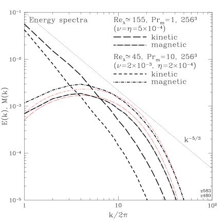
Figure 1: Energy spectra in simulations with $\text{Pr}_{\text{m}}=1$, $\text{Re}_{\lambda}\simeq 155$ and with $\text{Pr}_{\text{m}}=10$, $\text{Re}_{\lambda}\simeq 45$ (bold lines). The thin lines are our model-predicted spectra of the folded field component (normalized to have the same energy as the numerical spectra).

Let us consider the genesis of the magnetic field in isotropic MHD turbulence. As there is no mean field, all magnetic fields are fluctuations generated by the small-scale dynamo. This type of dynamo is a fundamental mechanism that amplifies magnetic energy in chaotic 3D flows with sufficiently large magnetic Reynolds numbers and $\text{Pr}_{\text{m}}\gtrsim 1$. The amplification is due to random stretching of the magnetic-field lines by the velocity field. During the kinematic (weak-field) stage of the dynamo, the magnetic energy grows exponentially in time, its spectrum is peaked at the resistive scale, $k_{\eta}\sim\text{Pr}_{\text{m}}^{1/2}k_{\nu}$, and grows self-similarly Kazantsev (1967); Kulsrud and Anderson (1992); Schekochihin et al. (2003). The growth rate is of the order of the turnover rate of the fastest eddies, which, in Kolmogorov turbulence, are the viscous-scale ones.

Although the bulk of the magnetic energy is at the resistive scale, the dynamo-generated fields are not at all randomly tangled, but rather organized in folds within which the field remains straight up to the scale of the flow and reverses direction at the resistive scale Ott (1998); Chertkov et al. (1999); Schekochihin et al. (2002a, 2003). One immediate implication of the folded field structure is the criterion for the onset of nonlinearity. For incompressible MHD, back reaction is controlled by the Lorentz tension force ${\bf B}\cdot\nabla{\bf B}\sim k_{\parallel}B^{2}$. This quantity depends on the parallel gradient of the field and does not know about direction reversals ($k_{\parallel}\sim k_{\nu}$ Schekochihin et al. (2002a)). Balancing ${\bf B}\cdot\nabla{\bf B}\sim{\bf u}\cdot\nabla{\bf u}$, we find that the back reaction is important when the magnetic energy becomes comparable to the energy of the viscous-scale eddies. Clearly, some form of nonlinear suppression of stretching motions at the viscous scale must then occur. However, the eddies at larger scales are still more energetic than the magnetic field and continue to stretch it at their (slower) turnover rate. When the field energy reaches the energy of these eddies, they are also suppressed and it is the turn of yet larger and slower eddies to exert dominant stretching. The folded structure is preserved with folds elongating to the size $\ell_{\text{s}}$ of the dominant stretching eddy. The key question is whether $\ell_{\text{s}}$ can increase all the way to the outer scale or stabilizes just above the viscous scale Schekochihin et al. (2002b).

The nonlinear suppression of stretching motions does not mean complete elimination of all turbulence: only the ${{\hat{\bf b\mkern-4.0mu}\mkern 4.0mu}{}}{{\hat{\bf b\mkern-4.0mu}\mkern 4.0mu}{}}:\nabla{\bf u}$ component of the velocity-gradient tensor leads to work being done against the Lorentz force and, therefore, must be suppressed. It is then natural to expect a local anisotropization of the velocity field. In this Letter, we demonstrate how a simple model accounting for this nonlinearly induced local anisotropy can produce solutions that are in remarkably good agreement with numerically observed magnetic-energy spectra.

The idea is to use the standard Kazantsev Kazantsev (1967) model velocity, Gaussian and white in time, $\langle u^{i}(t,{\bf x})u^{j}(t^{\prime},{\bf x}^{\prime})\rangle=\delta(t-t^{\prime})\kappa^{ij}({\bf x}-{\bf x}^{\prime})$, but let $\kappa^{ij}$ depend on the local direction of the magnetic field, ${{\hat{\bf b\mkern-4.0mu}\mkern 4.0mu}{}}={\bf B}/B$. In the Lagrangian frame (with local rotation transformed out), ${{\hat{\bf b\mkern-4.0mu}\mkern 4.0mu}{}}$ orients itself along the stretching Lyapunov direction of the flow, which stabilizes exponentially in time Goldhirsch et al. (1987). Therefore, in this frame, ${{\hat{\bf b\mkern-4.0mu}\mkern 4.0mu}{}}$ can be assumed to vary slowly with time. In the presence of one preferred direction defined by ${\hat{b}}^{i}{\hat{b}}^{j}$, the velocity correlator in ${\bf k}$ space has the following form

$$\kappa^{ij}({\bf k}) = \kappa^{\text{(i)}}(k,|\mu|)\bigl{(}\delta^{ij}-{\hat{k}}_{i}{\hat{k}}_{j}\bigr{)}+\kappa^{\text{(a)}}(k,|\mu|)\bigl{(}{\hat{b}}^{i}{\hat{b}}^{j}\bigr{.}$$ (3)

$$\bigl{.}+\,\,\mu^{2}{\hat{k}}_{i}{\hat{k}}_{j}-\mu{\hat{b}}^{i}{\hat{k}}_{j}-\mu{\hat{k}}_{i}{\hat{b}}^{j}\bigr{)},$$

where ${\hat{\bf k}}={\bf k}/k$, $\mu={\hat{\bf k}}\cdot{{\hat{\bf b\mkern-4.0mu}\mkern 4.0mu}{}}$. Let us ignore the spatial dependence of all quantities that vary at the flow scale and slower. The velocity will only enter via its gradient $u^{i}_{j}\equiv\partial_{j}u^{i}$, which is now a function of time only with statistics $\langle u^{i}_{m}(t)u^{j}_{n}(t^{\prime})\rangle=\delta(t-t^{\prime})\int d^{3}k\,k_{n}k_{m}\kappa^{ij}({\bf k})$. We can assume that ${{\hat{\bf b\mkern-4.0mu}\mkern 4.0mu}{}}$ also depends on time only, because it will always enter via the tensor ${\hat{b}}^{i}{\hat{b}}^{j}$, which varies at the scale of the flow (because of the folded structure of the magnetic field, the field’s curvature is very small Schekochihin et al. (2002a, 2003), so the fast spatial variation of ${{\hat{\bf b\mkern-4.0mu}\mkern 4.0mu}{}}$ is limited to sign reversals and cancels in ${\hat{b}}^{i}{\hat{b}}^{j}$). With these assumptions, the solution to Eq. (2) can be written as (cf. Zeldovich et al. (1984); Chertkov et al. (1999))

$${\bf B}(t,{\bf x})={{\hat{\bf b\mkern-4.0mu}\mkern 4.0mu}{}}(t)\int d^{3}k_{0}\,{\tilde{B}}(t,{\bf k}_{0})e^{i{\bf x}\cdot{\tilde{\bf k}}(t,{\bf k}_{0})},$$ (4)

where ${\tilde{\bf k}}(0,{\bf k}_{0})={\bf k}_{0}$ and

$$\partial_{t}{\tilde{B}} = {\hat{b}}^{i}{\hat{b}}^{m}u^{i}_{m}{\tilde{B}}-\eta{\tilde{k}}^{2}{\tilde{B}},$$ (5)

$$\partial_{t}{\tilde{k}}_{m} = -u^{i}_{m}{\tilde{k}}_{i},$$ (6)

$$\partial_{t}{\hat{b}}^{i} = {\hat{b}}^{m}u^{i}_{m}-{\hat{b}}^{l}{\hat{b}}^{m}u^{l}_{m}{\hat{b}}^{i}.$$ (7)

Equations (5–7) are a modification of the so-called zero-dimensional model of the dynamo Gruzinov et al. (1996). A closed equation can be obtained for the joint PDF of ${\tilde{B}}$, ${\tilde{\bf k}}$, and ${{\hat{\bf b\mkern-4.0mu}\mkern 4.0mu}{}}$, ${\cal P}({\tilde{B}},{\tilde{\bf k}},{{\hat{\bf b\mkern-4.0mu}\mkern 4.0mu}{}})=\delta(|{{\hat{\bf b\mkern-4.0mu}\mkern 4.0mu}{}}|^{2}-1)\delta({{\hat{\bf b\mkern-4.0mu}\mkern 4.0mu}{}}\cdot{\tilde{\bf k}})(4\pi^{2}{\tilde{k}})^{-1}P({\tilde{B}},{\tilde{k}})$, via an averaging procedure analogous to, e.g., the one in Ref. Schekochihin et al. (2002a). The magnetic-energy spectrum $M(k)=(1/2)\int_{0}^{\infty}dB\,B^{2}P(B,k)$ is then found to satisfy

$$\partial_{t}M = {1\over 8}\,\gamma_{\perp}{\partial\over\partial k}\biggl{[}(1+2\sigma_{\parallel})k^{2}{\partial M\over\partial k}\biggr{.}$$ (8)

$$\biggl{.}-\,\,(1+4\sigma_{\perp}+10\sigma_{\parallel})kM\biggr{]}$$

$$+\,\,2(\sigma_{\perp}+\sigma_{\parallel})\gamma_{\perp}M-2\eta k^{2}M,$$

where $\gamma_{\perp}=\int d^{3}k\,k_{\perp}^{2}\kappa_{\perp}$, $\sigma_{\perp}=(1/\gamma_{\perp})\int d^{3}k\,k_{\parallel}^{2}\kappa_{\perp}$, $\sigma_{\parallel}=(1/\gamma_{\perp})\int d^{3}k\,k_{\parallel}^{2}\kappa_{\parallel}$, $k_{\perp}=k(1-\mu^{2})^{1/2}$, $k_{\parallel}=k\mu$, $\kappa_{\perp}=(1/2)\bigl{(}\delta^{ij}-{\hat{b}}^{i}{\hat{b}}^{j}\bigr{)}\kappa^{ij}$, $\kappa_{\parallel}=(1/2){\hat{b}}^{i}{\hat{b}}^{j}\kappa^{ij}$, and $\kappa^{ij}$ is defined in Eq. (3). In the isotropic case, $\kappa^{\text{(i)}}=\kappa^{\text{(i)}}(k)$, $\kappa^{\text{(a)}}=0$, which gives $\sigma_{\perp}=2/3$, $\sigma_{\parallel}=1/6$. Equation (8) then reduces to the standard equation for the magnetic-energy spectrum in the kinematic dynamo Kazantsev (1967); Kulsrud and Anderson (1992). With a zero-flux boundary condition imposed at low $k$ Schekochihin et al. (2002b), Eq. (8) has an eigenfunction (in the limit $\eta\to+0$)

$$M(k)\simeq k^{s}e^{\gamma t}K_{0}(k/k_{\eta}),$$ (9)

where $K_{0}$ is the Macdonald function, $k_{\eta}=\bigl{[}(1+2\sigma_{\parallel})\gamma_{\perp}/16\eta\bigr{]}^{1/2}$, $s=2(\sigma_{\perp}+2\sigma_{\parallel})/(1+2\sigma_{\parallel})$, and $\gamma=(\gamma_{\perp}/8)\bigl{[}16(\sigma_{\perp}+\sigma_{\parallel})-(1+2\sigma_{\perp}+6\sigma_{\parallel})^{2}/(1+2\sigma_{\parallel})\bigr{]}$. As magnetic back-reaction makes velocity more anisotropic, the values of $\sigma_{\perp}$, $\sigma_{\parallel}$ drop compared to the isotropic case, and so does the growth rate $\gamma$ — until the dynamo is shut down (for a purely two-dimensional velocity, $\sigma_{\perp}=\sigma_{\parallel}=0$ and $\gamma=-\gamma_{\perp}/8$). Thus, saturation can be achieved purely by anisotropizing the statistics of the velocity field.

How do we make connection from a theory based on the $\delta$-correlated model velocity to the real turbulence, which has a finite correlation time? The simplest prescription is to get finite expressions for equal-time velocity correlators by replacing the $\delta$ function by $1/\tau_{\text{c}}$: $\langle u^{i}({\bf k})u^{j*}({\bf k})\rangle\equiv I^{ij}({\bf k})=\tau_{\text{c}}^{-1}\kappa^{ij}({\bf k})$. We take the correlation time $\tau_{\text{c}}$ of a given type of motions to be their “turnover time”: defining $I_{\perp}$ and $I_{\parallel}$ analogously to $\kappa_{\perp}$ and $\kappa_{\parallel}$, we write $k_{\perp}^{2}\kappa_{\perp}=C_{\perp\perp}\gamma_{\perp}^{-1}k_{\perp}^{2}I_{\perp}$, $k_{\parallel}^{2}\kappa_{\perp}=C_{\parallel\perp}(\sigma_{\perp}\gamma_{\perp})^{-1}I_{\perp}$, and $k_{\parallel}^{2}\kappa_{\parallel}=C_{\parallel\parallel}(\sigma_{\parallel}\gamma_{\perp})^{-1}I_{\parallel}$, where $C_{\perp\perp}$, $C_{\parallel\perp}$, $C_{\parallel\parallel}$ are adjustable constants. Then $\gamma_{\perp}=\bigl{[}C_{\perp\perp}\int d^{3}k\,k_{\perp}^{2}I_{\perp}\bigr{]}^{1/2}$, $\sigma_{\perp}=\bigl{[}(2/3)\int d^{3}k\,k_{\parallel}^{2}I_{\perp}\bigl{/}\int d^{3}k\,k_{\perp}^{2}I_{\perp}\bigr{.}\bigr{]}^{1/2}$, and $\sigma_{\parallel}=\bigl{[}(1/6)\int d^{3}k\,k_{\parallel}^{2}I_{\parallel}\bigl{/}\int d^{3}k\,k_{\perp}^{2}I_{\perp}\bigr{.}\bigr{]}^{1/2}$, where we have set $C_{\parallel\perp}=(2/3)C_{\perp\perp}$, $C_{\parallel\parallel}=(1/6)C_{\perp\perp}$ to ensure that $\sigma_{\perp}=2/3$ and $\sigma_{\parallel}=1/6$ in the isotropic case.

In order to model gradual anisotropization of the velocity statistics by the back reaction, we define the stretching wave number $k_{\text{s}}(t)$ such that the total magnetic energy $W(t)$ at time $t$ is equal to the energy of the hydrodynamic eddies at $k>k_{\text{s}}$ (before they feel the nonlinearity). We assume that the eddies at $k<k_{\text{s}}$ remain isotropic (unaffected by back reaction), while those at $k>k_{\text{s}}$ are two-dimensionalized. Specifically, for $k_{0}<k<k_{\text{s}}(t)$, let

$$4\pi k^{2}I^{\text{(i)}}(k,|\mu|)=E(k),\quad I^{\text{(a)}}(k,|\mu|)=0,$$ (10)

while for $k_{\text{s}}(t)<k<k_{\nu}$,

$$4\pi k^{2}I^{\text{(i)}}(k,|\mu|) = 2r_{\text{2D}}E(k)\,\delta(\mu),$$ (11)

$$4\pi k^{2}I^{\text{(a)}}(k,|\mu|) = 2\tilde{E}(k)\,\delta(\mu).$$ (12)

Here $k_{\text{s}}(t)$ is defined by $c_{2}\int_{k_{\text{s}}(t)}^{k_{\nu}}E(k)=W(t)$, $I^{\text{(i)}}$ and $I^{\text{(a)}}$ are coefficients of $I^{ij}$ analogous to $\kappa^{\text{(i)}}$ and $\kappa^{\text{(a)}}$ [Eq. (3)], $k_{0}$ and $k_{\nu}$ are the forcing and viscous wave numbers, $c_{2}$ and $r_{\text{2D}}$ are adjustable parameters. We take $E(k)=C_{\text{K}}\epsilon^{2/3}k^{-5/3}$ (with $C_{\text{K}}=1.5$) for $k\in[k_{0},k_{\nu}]$. The specific form of $E(k)$ will only affect details of the transient time evolution, not the saturated state. $\tilde{E}(k)$ will not figure in what follows, because it multiplies $\mu\delta(\mu)$ in all relevant expressions. Coefficients in Eq. (8) now depend on $W(t)$: a straightforward calculation gives

$$\gamma_{\perp}(t) = {6\over 5}\,{\bar{\gamma}}\biggl{[}1-{1\over(1+W_{0}/W_{\nu})^{2}}\biggr{]}^{-1/2}\bigl{[}\Gamma(t)\bigr{]}^{1/2},$$ (13)

$$\sigma_{\perp}(t) = 4\sigma_{\parallel}(t)={2\over 3}\,\biggl{[}{1\over(1+W(t)/W_{\nu})^{2}}\biggr{.}$$ (14)

$$\biggl{.}-\,\,{1\over(1+W_{0}/W_{\nu})^{2}}\biggr{]}^{1/2}\bigl{[}\Gamma(t)\bigr{]}^{-1/2},$$

$$\Gamma(t) = {1\over(1+W(t)/W_{\nu})^{2}}-{1\over(1+W_{0}/W_{\nu})^{2}}$$

$$+\,\,{5\over 4}\,r_{\text{2D}}\,\biggl{[}1-{1\over(1+W(t)/W_{\nu})^{2}}\biggr{]},$$

where ${\bar{\gamma}}=c_{1}\bigl{[}\int_{k_{0}}^{k_{\nu}}dk\,k^{2}E(k)\bigr{]}^{1/2}$, $c_{1}=\bigl{[}(5/18)C_{\perp\perp}\bigr{]}^{1/2}$, the viscous-eddy energy is $W_{\nu}/c_{2}=(3/2)C_{\text{K}}\epsilon^{2/3}k_{\nu}^{-2/3}$, and the total energy of the velocity field (before suppression) is $W_{0}/c_{2}=\int_{k_{0}}^{k_{\nu}}dk\,E(k)$. Equations (13–14) represent a generalization of the model first introduced in Ref. Schekochihin et al. (2002b) and reduce to it when $r_{\text{2D}}=0$. They include the effect of quasi-2D mixing of the folded magnetic fields by eddies whose stretching component has been suppressed. The spectrum of these mixing motions is modelled by Eq. (11), where $r_{\text{2D}}$ parametrizes the strength of the mixing relative to the original unsuppressed 3D turbulence.

The behavior of our model is easy to predict. The kinematic growth stage [$\gamma_{\perp}=(6/5){\bar{\gamma}}$, $\sigma_{\perp}=2/3$, $\sigma_{\parallel}=1/6$, and $s=3/2$, $\gamma=(3/4){\bar{\gamma}}$ in Eq. (9)] lasts until the total magnetic energy reaches the energy of the viscous-scale eddies, $W\sim W_{\nu}$. After that, the velocity is gradually anisotropized, stretching is weakened, but mixing continues at $k>k_{\text{s}}(t)$. A steady solution is reached as soon as $\sigma_{\perp}$ and $\sigma_{\parallel}$ have decreased enough to render $\gamma=0$ in Eq. (9). This gives $\sigma_{\perp}=4\sigma_{\parallel}\simeq 0.078$. The corresponding spectral exponent in the interval $k_{\nu}\ll k\ll k_{\eta}$ is $s\simeq 0.23$. This solution is valid in the limit $k_{\eta}\gg k_{\nu}$ ($\text{Pr}_{\text{m}}\gg 1$), but convergence in $\text{Pr}_{\text{m}}$ is only logarithmic. In practice, numerical solution of Eq. (8) shows that a scale separation of many decades is required for the scaling to be discernible. This is not achievable in direct numerical simulations. We have, therefore, solved Eq. (8) with the same parameters as those used in our simulations Schekochihin et al. (2003). There are three adjustable constants: $c_{1}$, $c_{2}$, and $r_{\text{2D}}$. The solution does not, however, depend very strongly on them: $c_{2}$ is irrelevant as it amounts to overall rescaling of energy, $r_{\text{2D}}$ has to vary by an order of magnitude to cause significant change, and even $c_{1}$ (which affects the value of $k_{\eta}$) does not require very fine tuning. We have compared the model solutions for the same fixed values $c_{1}=1/3$ and $r_{\text{2D}}=4/5$ with the (normalized) spectra obtained in numerical simulations. A sequence of runs with large $\text{Pr}_{\text{m}}$ and low Re (the so-called viscosity-dominated limit: a necessary compromise at current resolutions Schekochihin et al. (2003)) is well fitted by our model in both kinematic (not shown) and nonlinear (Fig. 2) regimes (except at $k/2\pi=1,~{}2$, where finite-box effects are important). Note that the velocity field in these runs is random [because of random forcing, Eq. (1)], but, unlike in real turbulence, spatially smooth and one-scale.

It is extraordinary that our minimal model has reproduced non-asymptotic numerical spectra so well. We do not claim that it constitutes a quantitative theory of nonlinear dynamo. It does, however, provide a simple demonstration that the available numerical data is consistent with magnetic-energy spectra exhibiting a very flat positive spectral exponent in the interval $k_{\nu}\ll k\ll k_{\eta}$ if sufficiently large scale separations were resolved.

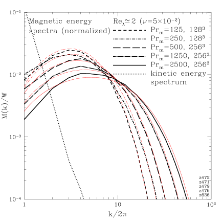
Figure 2: The bold lines are the normalized saturated energy spectra for simulations in the viscosity-dominated regime Schekochihin et al. (2003). The thin lines are the spectra predicted by our model.

It is clear that the viscosity-dominated simulations (low Re) are described very well by our model. The case $\text{Re}\gg 1$, $\text{Pr}_{\text{m}}\gg 1$ is much harder to tackle. If mixing by velocities at $k\in[k_{\text{s}},k_{\nu}]$ remains efficient [as implied by our 2D approximation (11–12)], then $k_{\text{s}}$ stabilizes at a value $\sim k_{\nu}$ and saturated magnetic energy scales with Re as the energy of the viscous eddies, $\langle B^{2}\rangle\sim\text{Re}^{-1/2}\langle u^{2}\rangle$. This outcome does not appear to be borne out by the available numerical evidence, which rather suggests $\langle B^{2}\rangle\lesssim\langle u^{2}\rangle$ Haugen et al. (2003) (though limited resolutions preclude a definitive statement). In our runs with $\text{Pr}_{\text{m}}=10$ and Taylor-microscale Reynolds number $\text{Re}_{\lambda}\simeq 45$ ($\text{Re}\sim 100$) and with $\text{Pr}_{\text{m}}=1$, $\text{Re}_{\lambda}\simeq 155$ ($\text{Re}\sim 400$), our model in its present form overestimates the magnetic energy at large $k$, but underestimates it at low $k$ (Fig. 1): an indication of too much mixing in the model . Indeed, when $\text{Re}\gg 1$, the nature of the anisotropized velocities in the interval $[k_{\text{s}},k_{\nu}]$ can be very different from the interchange-like motions that give the 2D mixing in the viscosity-dominated case. In Ref. Schekochihin et al. (2002b), we argued that the interval $[k_{\text{s}},k_{\nu}]$ is populated by Alfvén waves that propagate along the folds. The saturated spectrum is then the result of a superposition of waves and folds (which accounts for the large amount of small-scale magnetic energy). Since the Alfvén waves are dissipated by viscosity, they can only exist if the stretching scale becomes much larger than the viscous scale: possibly as large as the outer scale ($k_{\text{s}}\sim k_{0}$, cf. Schekochihin et al. (2003)). This is only allowed if the waves do not mix magnetic field as efficiently as the interchange motions do. For our model, the required modification would be that the mixing rate $\gamma_{\perp}$ should decrease with $k_{\text{s}}$. The dynamo saturation would then be due to a balance between stretching and mixing by partially anisotropized motions at the stretching scale.

Detecting Alfvén waves along folds is a challenge for future numerical work. The main conclusion of the present study is that the nonlinear dynamo in a random one-scale flow can be described by a simple model where saturation is achieved via partial anisotropization of the ambient velocity, a result quantitatively supported by agreement with direct numerical simulations.

References

Batchelor (1950)
G. K. Batchelor,
Proc. R. Soc. London A 201,
405 (1950).
Widrow (2002)
L. M. Widrow,
Rev. Mod. Phys. 74,
775 (2002).
Schekochihin et al. (2003)
A. A. Schekochihin et al.
(2003), astro-ph/0312046.
Iroshnikov (1964)
P. S. Iroshnikov,
Sov. Astron. 7,
566 (1964).
Kraichnan (1965)
R. H. Kraichnan,
Phys. Fluids 8,
1385 (1965).
Goldreich and Sridhar (1995)
P. Goldreich and
S. Sridhar,
Astrophys. J. 438,
763 (1995).
Maron and Goldreich (2001)
J. Maron and
P. Goldreich,
Astrophys. J. 554,
1175 (2001).
Haugen et al. (2003)
N. E. L. Haugen et al.,
Astrophys. J. 597,
L141 (2003).
Kazantsev (1967)
A. P. Kazantsev,
Zh. Eksp. Teor. Fiz. 53,
1806 (1967), [Sov. Phys.–JETP 26, 1031 (1968)].
Kulsrud and Anderson (1992)
R. M. Kulsrud and
S. W. Anderson,
Astrophys. J. 396,
606 (1992).
Ott (1998)
E. Ott, Phys. Plasmas 5, 1636
(1998).
Chertkov et al. (1999)
M. Chertkov et al.,
Phys. Rev. Lett. 83,
4065 (1999).
Schekochihin et al. (2002a)
A. Schekochihin et al.,
Phys. Rev. E 65,
016305 (2002a).
Schekochihin et al. (2002b)
A. A. Schekochihin et al.,
New J. Phys. 4,
84 (2002b).
Goldhirsch et al. (1987)
I. Goldhirsch et al.,
Physica D 27,
311 (1987).
Zeldovich et al. (1984)
Y. B. Zeldovich et al.,
J. Fluid Mech. 144,
1 (1984).
Gruzinov et al. (1996)
A. Gruzinov et al.,
Phys. Rev. Lett. 77,
4342 (1996).