To appear in The Astrophysical Journal
Scattering by Interstellar Dust Grains. II. X-Rays

Abstract

Scattering and absorption of X-rays by interstellar dust is calculated for a model consisting of carbonaceous grains and amorphous silicate grains. The calculations employ realistic dielectric functions with structure near X-ray absorption edges, with resulting features in absorption, scattering, and extinction.

Differential scattering cross sections are calculated for energies between 0.3 and 10 keV. The median scattering angle is given as a function of energy, and simple but accurate approximations are found for the X-ray scattering properties of the dust mixture, as well as for the angular distribution of the scattered X-ray halo for dust with simple spatial distributions. Observational estimates of the X-ray scattering optical depth are compared to model predictions. Observations of X-ray halos to test interstellar dust grain models are best carried out using extragalactic point sources.

1 Introduction

Interstellar grains can absorb and scatter X-rays. The scattering, typically through small angles, results in a “halo” of scattered X-rays within $\sim 1^{\circ}$ of an X-ray source (Overbeck 1965; Hayakawa 1970; Martin 1970). The observed properties of these X-ray halos provide a test of interstellar grain models.

The nature of interstellar grains remains uncertain (see Draine 2003a, and references therein). This paper will examine X-ray scattering and absorption for a grain model consisting of two separate grain populations – carbonaceous grains and silicate grains. With the grains approximated by homogeneous spheres with the size distribution found by Weingartner & Draine (2001; hereafter WD01), this grain model is consistent with the observed interstellar extinction law, the observed infrared emission from interstellar dust (Li & Draine 2001, 2002), and the X-ray scattering halo observed around Nova Cygni 1992 (Draine & Tan 2003). The carbonaceous grains are assumed to be graphitic when the grains are large, extending down to very small sizes with the smallest grains being individual polycyclic aromatic hydrocarbon molecules. The scattering is dominated by grains with radii $a\gtrsim 100\,{\rm\AA}$, containing $\gtrsim 10^{6}$ atoms; carbonaceous grains in this size range are modelled using the optical properties of graphite.

The primary objective of this paper is to calculate the X-ray scattering and absorption properties of this dust model, and to make these results available for comparison with observations. The paper has three relatively independent parts, and readers may wish to proceed directly to the material of interest to them.

The first part of this paper – §2 – is concerned with the dielectric functions of graphite and MgFeSiO₄ from infrared to X-ray energies. The resulting dielectric functions satisfy the Kramers-Kronig relations as well as the oscillator strength sum rule.

The second part of the paper – §§3–4 – examines the X-ray scattering properties of interstellar dust, including structure near X-ray absorption edges. The angular distribution of the scattered X-rays is discussed: the median scattering angle $\theta_{s,50}$ is found as a function of energy, and a simple analytic approximation to the differential scattering cross section is presented. In §4 we provide analytic approximations for the intensity distribution in X-ray scattering halos for simple dust density distributions.

The final part of the paper, §5, discusses observations of X-ray scattering halos, and values of total scattering cross section derived from these observations. We conclude that the observational situation is unclear at this time, due to the combined effects of instrumental limitations and uncertainties in the spatial distribution of the dust, but the silicate/carbonaceous grain model appears to be consistent with the overall body of observational data. Future observations using extragalactic point sources could transcend the uncertainties concerning the dust spatial distribution.

The principal results are summarized in §6

2 Dielectric Function

Our objective here is to obtain continuous complex dielectric functions $\epsilon(\omega)=\epsilon_{1}+i\epsilon_{2}$ which can be used to calculate scattering and absorption by these grains from the submm to hard X-rays. For material at LTE (i.e., no population inversions), the dielectric function must have $\epsilon_{2}\geq 0$. Causality requires that the dielectric function must satisfy the Kramers-Kronig relations (Landau & Lifshitz 1960), in particular

$$\epsilon_{1}(\omega)=1+\frac{2}{\pi}P\int_{0}^{\infty}\frac{\epsilon_{2}(x)xdx}{x^{2}-\omega^{2}}~{}~{}~{},$$ (1)

where $P$ indicates that the principal value is to be taken. We will proceed by first specifying $\epsilon_{2}(\omega)$ at all frequencies, and then obtaining $\epsilon_{1}(\omega)$ using eq. (1).

In addition to satisfying the Kramers-Kronig relations, the dielectric function must obey the sum rule (Altarelli et al. 1972)

$$\int_{0}^{\infty}\omega\epsilon_{2}(\omega)d\omega=\frac{2\pi^{2}e^{2}}{m_{e}}\sum_{j}n_{j}Z_{j}~{}~{}~{},$$ (2)

where $n_{j}$ is the number density and $Z_{j}$ is the number of electrons in element $j$. Thus we may define the effective number of electrons per molecule

$$n_{\rm eff}(\omega)\equiv\frac{m_{e}V_{0}}{2\pi^{2}e^{2}}\int_{0}^{\omega}x\epsilon_{2}(x)dx~{}~{}~{},$$ (3)

where $V_{0}$ is the volume per molecule, and $n_{\rm eff}(\infty)=$ the total number of electrons per molecule.

Ideally, $\epsilon_{2}(\omega)$ would be measured in the laboratory for the materials of interest. At energies below $\sim$20-30 eV the optical constants can be characterized using transmission and ellipsometric studies, but calibrated experimental measurements are usually unavailable at X-ray energies. At high energies $\hbar\omega\gtrsim 100\,{\rm eV}$, $\epsilon_{2}(\omega)$ for a material can be approximated by summing the atomic absorption cross sections of the constituent atoms:

$$\epsilon_{2}(\omega)\approx\frac{c}{\omega}\sum_{j}n_{j}\sum_{s}\sigma_{j,s}(\omega)~{}~{}~{},$$ (4)

where $\sigma_{j,s}$ is the atomic absorption cross section contributed by electronic shell $s$ of element $j$. Eq. (4) assumes that $|\epsilon-1|\ll 1$, which is valid at X-ray energies.

At energies well above the photoionization threshold for shell $s$, atomic photoionization is to high momentum free electron states which will have counterparts in the solid, and we can approximate $\sigma_{j,s}$ by the atomic photoionization cross section fitting functions $\sigma_{j,s}^{pi}(\omega)$ estimated for inner shell electrons by Verner & Yakovlev (1995), and for outer-shell electrons by Verner et al. (1996), as implemented in the Fortran routine phfit2.f (Verner 1996). Near threshold, however, the photoabsorption cross section $\sigma_{j,s}(\omega)$ depends on the band structure of the solid, leading to “Near Edge X-ray Absorption Fine Structure” (NEXAFS), which could in principle permit identification of interstellar grain materials through observations of X-ray absorption and scattering near absorption edges (Martin 1970; Woo 1995).

2.1 Graphite

We will assume that interstellar grains are constructed primarily from two distinct substances: carbonaceous material and amorphous silicate material. In ultrasmall grains, containing less than $\sim 10^{5}$ atoms, the carbonaceous material has the properties of polycyclic aromatic hydrocarbon molecules. Because of their small size, scattering by these grains is negligible, and the IR-optical-UV absorption can be calculated using absorption cross sections estimated for PAH molecules or ions (Draine & Li 2001; Li & Draine 2001).

In the larger carbonaceous grains, the nature of the carbon material is less certain. The carbon atoms could be arranged in a graphitic structure (pure $sp^{2}$ bonding) or there might be a mixture of $sp^{2}$ (graphitic) and $sp^{3}$ (diamond-like) bonding, perhaps also with some aliphatic (chainlike) hydrocarbon material as well. We will assume that the optical response of the carbonaceous material in the grains containing $\gtrsim 10^{5}$ atoms can be approximated by graphite, with density $\rho=2.2\,{\rm g}\,{\rm cm}^{-3}$.

Graphite is anisotropic, with the crystal “c axis” normal to the basal plane. In a cartesian coordinate system with $\hat{\bf z}\parallel c$, the dielectric tensor is diagonal with eigenvalues $(\epsilon_{\perp},\epsilon_{\perp},\epsilon_{\parallel})$.

The dielectric functions $\epsilon_{\perp}$ and $\epsilon_{\parallel}$ were estimated by Draine & Lee (1984, hereafter DL84) and Laor & Draine (1993). For $E<22\,{\rm eV}$ we continue to use $\epsilon_{\parallel,2}$ from DL84, while for $E>22\,{\rm eV}$ we use eq. (4) to estimate $\epsilon_{\parallel,2}$. For $E<35\,{\rm eV}$ we use $\epsilon_{\perp,2}$ estimated by DL84, while for $E>35\,{\rm eV}$ we use eq. (4) to estimate $\epsilon_{\perp,2}$. Our final $\epsilon_{\perp,2}$ and $\epsilon_{\parallel,2}$ are shown in Figures 1 and 3.

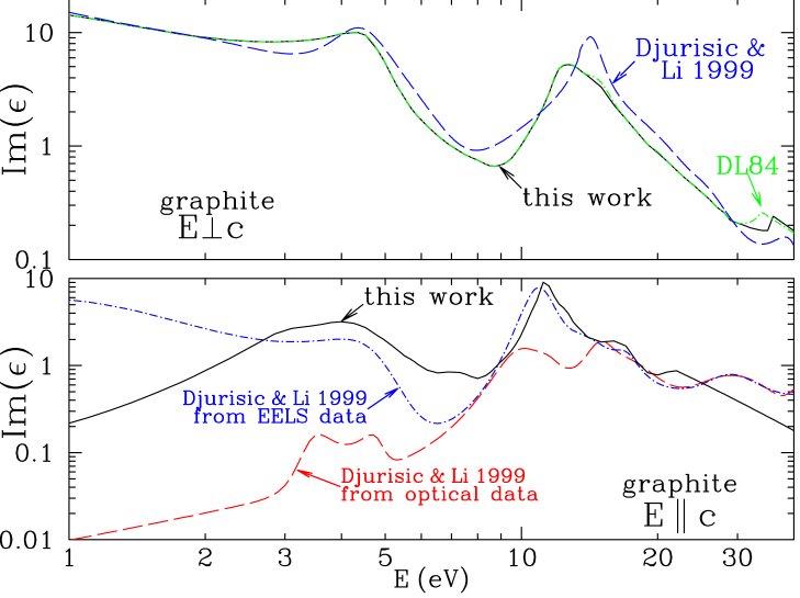
Figure 1: ${\rm Im}(\epsilon)$ for graphite at $E<40\,{\rm eV}$ (see text). The $\epsilon_{\perp}$ adopted here is equal to $\epsilon_{\perp}$ adopted by DL84 below 30 eV. Also shown, for comparison, are estimates for $\epsilon_{\perp}$ and $\epsilon_{\parallel}$ by Djurisic & Li (1999).

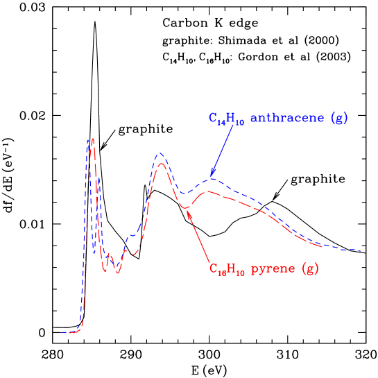
Figure 2: Oscillator strength for absorption near the carbon K edge in gaseous anthracene and pyrene (Gordon et al. 2003), and for graphite (Shimada et al. 2000, with normalization discussed in text).

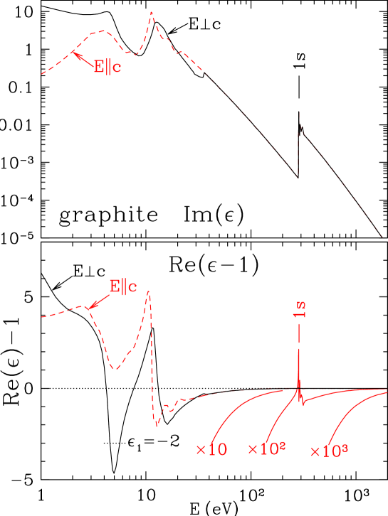
Figure 3: ${\rm Im}(\epsilon)$ and ${\rm Re}(\epsilon-1)$ for graphite from 1 eV to 2 keV.

Djurisic & Li (1999) recently reestimated $\epsilon_{\perp}$ and $\epsilon_{\parallel}$ for $\hbar\omega<40\,{\rm eV}$ by fitting a model to the available experimental evidence. Their estimate for ${\rm Im}(\epsilon_{\perp})$ is shown in Figure 1. We see that it is generally similar to the DL84 dielectric function, although with a pronounced peak at $\sim 14\,{\rm eV}$ in place of the broader feature peaking at $\sim 12\,{\rm eV}$ in the DL84 estimate of $\epsilon_{\perp}$.

For $E\parallel c$, however, Djurisic & Li concluded that optical ellipsometric measurements are inconsistent with the dielectric function estimated from electron energy loss spectroscopy (EELS). Djurisic & Li obtained $\epsilon_{\parallel}(\omega)$ from the optical measurements and then independently from the EELS data. These two estimates for $\epsilon_{\parallel}$ – which differ substantially – are shown in Figure 1. The Djurisic & Li estimate based on EELS data is fairly similar to the DL84 estimate for $\epsilon_{\parallel}$ (which was based in part on experimental papers using EELS). Given the inconsistencies among the different experimental investigations, $\epsilon_{\parallel}$ in the optical and UV should be regarded as uncertain.

For carbon, the only X-ray feature is the carbon K edge. We use the measured K edge X-ray absorption profile for graphite from Shimada et al. (2000) for 282 - 310 eV. Shimada et al. did not determine the absolute absorption strength. We fix the amplitude such that the oscillator strength between 282 and 320 eV is 0.38, and we smoothly connect to join the Verner & Yakovlev (1995) photoionization cross section at 320 eV. In Figure 2 we show the oscillator strength density

$$\frac{df}{dE}=\frac{m_{e}V_{0}}{\pi e^{2}h}\omega\epsilon_{2}(\omega)$$ (5)

near the carbon K edge for graphite, and, for comparison, for gas phase anthracene and pyrene (Gordon et al. 2003).

In Figure 3 we show $\epsilon_{\parallel,2}$ and $\epsilon_{\perp,2}$ from the optical to the X-ray region. Figure 3 shows $\epsilon_{\parallel,1}$ and $\epsilon_{\perp,1}$ obtained using eq. (1).

A useful check on the validity of the dielectric function is provided by eq. (3). Figure 4 shows that $n_{\rm eff}(\omega)\approx 4$ just below the onset of K shell absorption, and $n_{\rm eff}(\omega\rightarrow\infty)\rightarrow 6$, as expected for carbon.

2.2 Silicate

We will assume that the silicate material has an olivine composition, Mg_2xFe_2(1-x)SiO₄. Mg and Fe are approximately equally abundant in the ISM, and both reside primarily in interstellar grains. It is therefore reasonable to take the silicate grain composition to be MgFeSiO₄, although it is possible that, for example, some of the Fe may be another chemical form. MgFeSiO₄ olivine has a density 3.8$\,{\rm g}\,{\rm cm}^{-3}$, intermediate between the densities of forsterite (Mg₂SiO₄, 3.27$\,{\rm g}\,{\rm cm}^{-3}$) and fayalite (Fe₂SiO₄, 4.39$\,{\rm g}\,{\rm cm}^{-3}$), with a molecular volume $V_{0}=7.5\times 10^{-23}\,{\rm cm}^{3}$.

For $h\nu<18\,{\rm eV}$ we will adopt $\epsilon_{2}$ previously obtained by Draine & Lee (1984) for “astronomical silicate”, but with the following modifications to $\epsilon_{2}$:

1. the crystalline olivine feature at $\lambda^{-1}=6.5\micron^{-1}$ – not seen in interstellar extinction or polarization (Kim & Martin 1995) – has been excised with the oscillator strength redistributed over frequencies between 8 and 10$\micron^{-1}$ (Weingartner & Draine 2001)

2. at $\lambda>250\micron$, $\epsilon_{2}(\omega)$ has been modified slightly, as described by Li & Draine (2001). For $250<\lambda<1100\micron$ the revised $\epsilon_{2}$ is within $\pm 12\%$ of $\epsilon_{2}$ adopted by DL84.

Above 30 eV, we use eq. (4) to estimate $\epsilon_{2}$ from atomic photoabsorption cross sections, except near absorption edges (see below). Between 18 and 30 eV, $\epsilon_{2}$ is chosen to provide a smooth join between $\epsilon_{2}$ from DL84 and $\epsilon_{2}$ estimated from the atomic photoabsorption cross sections.

The threshold energy for photoionization from the K shell of atomic oxygen is 544.0 eV for ionization to O II $1s2s^{2}2p^{4}(^{4}{\rm P})$, and 548.9 eV for ionization to O II $1s2s^{2}2p^{4}(^{2}{\rm P})$; the strong $1s-2p$ absorption line, with FWHM $\approx 0.14\,{\rm eV}$, lies at 527.0 eV (Stolte et al. 1997). From the theoretical line profile of McLaughlin & Kirby (1998), the $1s-2p$ transition has an oscillator strength $f\approx 0.10$.

X-ray spectroscopy of several galactic X-ray sources using the Chandra X-Ray Observatory has detected a strong and narrow absorption line at 527.5 eV which must be the O I $1s-2p$ transition, and a nearby absorption feature at 530.8 eV, with FWHM $\sim$1.0eV (Paerels et al. 2001; Schulz et al. 2002; Takei et al. 2002). Paerels et al. and Schulz et al. suggest that the 530.8 eV feature is due to iron oxides, possibly Fe₂O₃. However, O II is expected to have $1s-2p$ absorption at approximately this energy, and the interstellar O II abundance is probably large enough that the resulting absorption feature should be conspicuous. It therefore seems likely that the observed narrow feature at 530.8 eV is (at least primarily) O II $1s-2p$.

In the absence of published X-ray absorption spectra for amorphous silicates, we estimate the oxygen K edge absorption using measurements on crystalline olivines. Li et al. (1995) have measured Mg K edge and Si K edge absorption for forsterite Mg₂SiO₄, and Henderson et al. (1995) have measured Fe K edge absorption in fayalite Fe₂SiO₄. We adopt these profiles for the corresponding K edges in amorphous olivine MgFeSiO₄, with the absorption profile strengths adjusted to match the Verner et al. photoionization cross sections for the corresponding atoms well above threshold.

Fe L_2,3 edge spectra for a number of minerals have been studied recently by van Aken & Liebscher (2002). The L₂ edge corresponds to the remaining $2p^{5}$ electrons in a ²P_3/2 term, and the L₃ edge when they are in a ²P_1/2 term. The Fe in olivine is 100% Fe²⁺. The spin-orbit splitting for Fe²⁺ produces a 12.8 eV separation between the L₂ and L₃ maxima (van Aken & Liebscher 2002), with the L₂ peak at 721.3 eV and the L₃ peak at 708.1 eV. Following van Aken & Liebscher, we model the near-edge absorption in olivine by

$$\sigma_{L_{2,3}} = \sigma_{0}\left\{\frac{2}{3\pi}\left[\arctan\left(\frac{\pi}{w_{a}}(E-E_{a})\right)+\frac{\pi}{2}\right]+\frac{1}{3\pi}\left[\arctan\left(\frac{\pi}{w_{b}}(E-E_{b})\right)+\frac{\pi}{2}\right]\right.$$ (6)

$$\left.+\sum_{i=1}^{4}A_{i}\exp\left[-\left(\frac{E-E_{j}}{w_{j}}\right)^{2}\right]\right\}~{}~{}~{},$$

with $E_{a}=708.65\,{\rm eV}$, $E_{b}=721.65\,{\rm eV}$, and $w_{a}=w_{b}=1\,{\rm eV}$. The gaussian components are located at $E_{1}=707.8\,{\rm eV}$, $E_{2}=710.5\,{\rm eV}$, $E_{3}=720.6\,{\rm eV}$, and $E_{4}=723.3\,{\rm eV}$. van Aken & Liebscher do not give values for the widths of the gaussians, but inspection of their Fig. 1 suggests $w_{1}=w_{2}=w_{3}=w_{4}=1.25\,{\rm eV}$. Minerals with 100% Fe²⁺ have $A_{1}/A_{2}\approx A_{3}/A_{4}\approx 5$, and $A_{3}/A_{1}\approx 0.28$. For 100% ferrous Fe we estimate $A_{1}\approx 6$ from the spectrum of ilmenite FeTiO₃ in van Aken, Liebscher & Styrsa (1998). To determine the normalization $\sigma_{0}$, we require that eq. (6) match the Verner et al. cross section at 800 eV.

For some absorption edges no measurements are available for appropriate minerals. Since the near-edge absorption is proportional to the density of electronic states above the Fermi surface, the near edge spectra for different elements in a compound show considerable similarity in the dependence on energy, but with displacements in energy due to the different binding energies of the electron being excited. We use the Si K edge in forsterite Mg₂SiO₄ (Li et al. 1995), shifted in energy by $\Delta E=-1308\,{\rm eV}$ [the difference in K edge ionization thresholds for Si I (1846 eV) and O I (538 eV)] to determine the O K edge absorption profile up to 575 eV. This results in onset of O 1s absorption at $\sim$527.8 eV, and an O 1s absorption peak at 537.6 eV. The absolute absorption coefficient is fixed by requiring that the absorption at 575 eV match that calculated from the atomic photoionization cross sections.

A similar approach is taken for the other absorption edges, using measured profiles for Mg K edge and Si K edge absorption in forsterite Mg₂SiO₄ (Li et al. 1995), and Fe K edge absorption in fayalite Fe₂SiO₄ (Henderson et al. 1995) (see Table 1).

Although this procedure is not expected to provide accurate estimates of the near-edge absorption spectra for amorphous silicates, the provisional near-edge absorption profiles so obtained will provide a realistic example of the kind of near-edge absorption and scattering expected from interstellar grains.

Table 1: X-ray Edge Absorption Parameters

material	shell	$E_{min}$	$E_{peak}$	$\sigma_{peak}$	adopted	$\Delta E$
		(eV)	(eV)	Mb	profile	(eV)	ref
graphite	C $1s~{}(K)$	282	285.4	3.84	graphite	0
olivine	O$1s~{}(K)$	527.8	537.6	1.78	Mg2SiO4 Mg K	-1308.0
olivine	Mg$1s~{}(K)$	1300.8	1310.6	0.80	Mg2SiO4 Mg K	0
olivine	Mg $2s~{}(L_{1})$	83.8	93.6	2.07	Mg2SiO4 Mg K	-1752.0
olivine	Mg $2p~{}(L_{2,3})$	44.7	54.5	15.7	Mg2SiO4 Mg K	-1791.1
olivine	Si $1s~{}(K)$	1835.8	1845.6	0.50	Mg2SiO4 Si K	0
olivine	Si $2s~{}(L_{1})$	145.8	155.6	1.67	Mg2SiO4 Si K	-1690.0
olivine	Si $2p~{}(L_{2,3})$	95.8	105.6	18.0	Mg2SiO4 Si K	-1740.0
olivine	Fe $1s~{}(K)$	7105	7123	.0544	Fe2SiO4 Fe K	0
olivine	Fe $2s~{}(L_{1})$	838	856	0.186	Fe2SiO4 Fe K	-6267.
olivine	Fe $2p(L_{2})$	705	720.6	2.46	Fe2+ minerals Fe L2	0
olivine	Fe $2p(L_{3})$	705	707.8	6.30	Fe2+ minerals Fe L3	0
olivine	Fe $3s~{}(M_{1})$	85	103	0.338	Fe2SiO4 Fe K	-7020
olivine	Fe $3p~{}(M_{2,3})$	47	65	1.41	Fe2SiO4 Fe K	-7058

Figure 5 shows ${\rm Re}(\epsilon)$ obtained from ${\rm Im}(\epsilon)$ using eq. (1). Figure 4 provides a check on the adopted dielectric function: $\lim_{\omega\rightarrow\infty}n_{\rm eff}=84.01$, in agreement with the value of 84 expected theoretically for MgFeSiO₄.

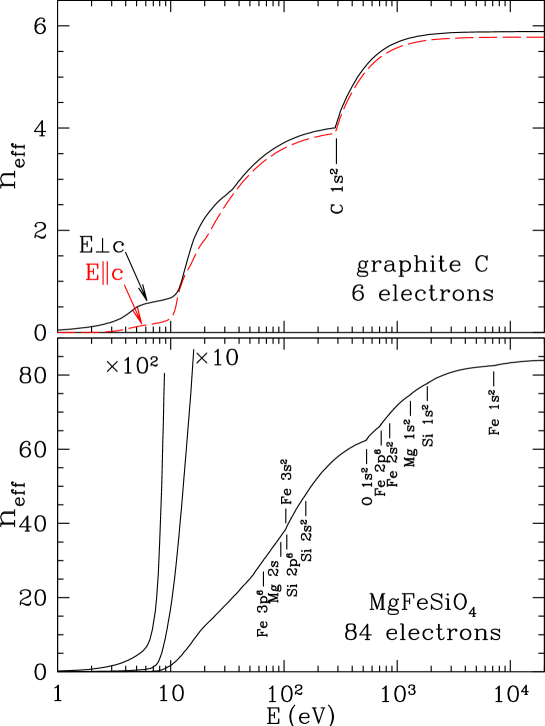
Figure 4: Effective number of electrons $n_{\rm eff}$ as a function of photon energy for graphite and MgFeSiO₄.

Figure 5: ${\rm Im}(\epsilon)$ and ${\rm Re}(\epsilon-1)$ for silicate MgFeSiO₄.

3 Cross Sections for X-Ray Absorption and Scattering

Adopting the dielectric functions discussed in §2, we calculate the scattering and absorption for the WD01 dust grain mixture. We use the Mie scattering theory program of Wiscombe (1980, 1996) for $x=2\pi a/\lambda<2\times 10^{4}$, and anomalous diffraction theory (van de Hulst 1957) for $x>2\times 10^{4}$. Anomalous diffraction theory provides an excellent approximation at the X-ray energies where $x=5067(a/\micron)(E/\,{\rm keV})>2\times 10^{4}$ (see Figure 7 of Draine & Tan 2003).

The scattering and extinction cross section calculated for the dust mixture is shown in Fig. 6 for 0.1–10 keV X-rays, with the six strongest absorption edges shown in Fig. 7. Also shown is the absorption per H atom due to gas-phase absorption calculated using phfit2.f (Verner 1996), with interstellar gas-phase abundances. At energies $13.6<E\lesssim 250\,{\rm eV}$, absorption by neutral H and He is very strong, making it difficult to observe the dust absorption and scattering. Above 250 eV, however, observations of extinction and scattering by dust become feasible for suitably bright sources on sightlines with sufficient dust columns. At $E\gtrsim 800\,{\rm eV}$ the extinction is primarily due to dust grains.

As seen in Figure 7, the calculated scattering cross sections show conspicuous structure in the vicinity of the major absorption edges. This occurs because at X-ray energies ${\rm Re}(\epsilon-1)$ tends to be negative, and an absorption feature increases ${\rm Re}(\epsilon)$ (reducing $|\epsilon-1|$) just below the absorption feature, and decreases ${\rm Re}(\epsilon)$ (increasing $|\epsilon-1|$) just above the feature. Since the scattering is approximately proportional to $|\epsilon-1|^{2}$, this results in a reduction in scattering below an absorption feature, and an increase in scattering above. This argument applies to 5 of the 6 absorption edges in Fig. 7; the exception is the C K edge, for which $\epsilon-1$ actually becomes positive below the absorption edge, with a local peak in scattering just below the K edge.

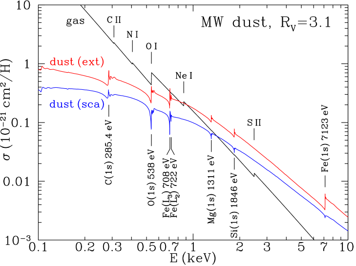
Figure 6: X-ray extinction and scattering cross section per H nucleon due to dust, and absorption due to gas. Data available at http://www.astro.princeton.edu/$\sim$draine/dust.html

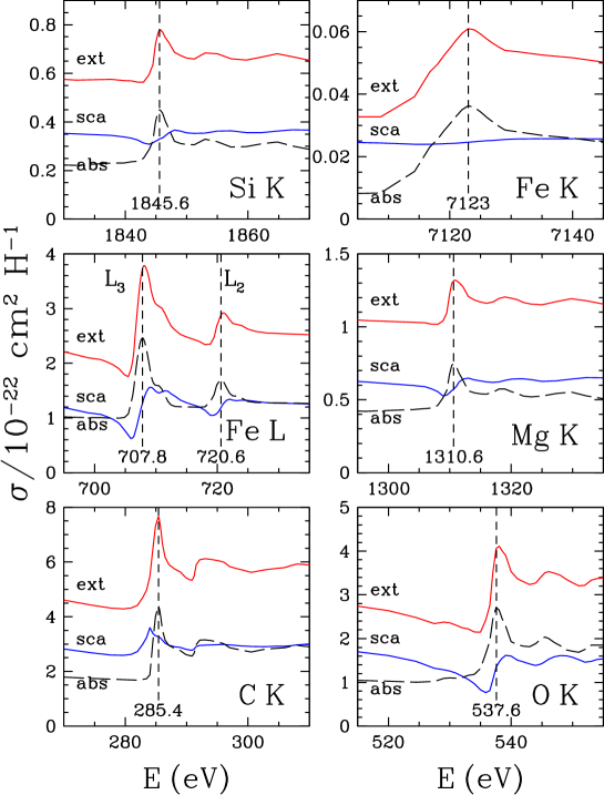
Figure 7: X-ray extinction and scattering cross section per H nucleon near major absorption edges.

For the lower-energy absorption edges (C K, O K, Fe L_2,3) there is significant variation in the scattering cross section near the absorption edge. As a result, the extinction profile is not the same as the absorption profile. In the case of the O K edge, the extinction peak is at 538.0 eV, whereas the absorption peak is at 537.6 eV. The energy-dependence of the scattering optical depth can be determined by dividing the spectrum of the scattered X-rays by the spectrum of the point source component. If this can be done with a signal-to-noise ratio $\gtrsim 10$ for $\sim 2\,{\rm eV}$ bins, one should observe the structure in $\sigma_{\rm sca}$ seen near 285, 538, and 708 eV in Figure 7.

At X-ray energies, the dielectric functions of grain materials become close to unity (see Figures 3 and 5), the wavelength is small compared to the typical grain radius, and the grains are very strongly forward-scattering. The quantity

$$\frac{d\sigma_{\rm sca}}{d\ln\Omega}=\Omega\frac{d\sigma}{d\Omega}=2\pi(1-\cos\theta)\frac{d\sigma}{d\Omega}\approx\pi\theta^{2}\frac{d\sigma}{d\Omega}~{}~{}~{}$$ (7)

is proportional to the number of scattered photons per logarithmic interval of scattering angle; the location of the peak shows the “typical” scattering angle. Figure 8 shows $\pi\theta^{2}d\sigma/d\Omega$ for the WD01 dust mixture for selected energies from 0.3 keV to 10 keV.

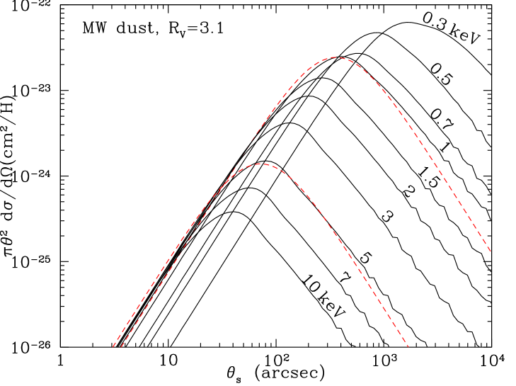
Figure 8: $2\pi\theta^{2}d\sigma/d\Omega$ versus scattering angle $\theta_{s}$ at selected energies. This function peaks at approximately the median scattering angle. The broken curves show eq. (11) for $E=1.0$ and $5.0\,{\rm keV}$.

Let $\theta_{s,50}(E)$ be the median scattering angle for photons of energy $E$. Figure 9 shows $\theta_{s,50}(E)$ for the WD01 dust mixture; comparison with Fig. 8 shows that, as expected, the median scattering angle $\theta_{s,50}$ is very nearly the same as the angle where $\pi\theta^{2}d\sigma/d\Omega$ peaks. Also shown in Fig. 9 are the 10th and 90th percentile scattering angles, $\theta_{s,10}$ and $\theta_{s,90}$, corresponding to 10% and 90% enclosed power. Note that to a very good approximation,

$$\theta_{s,10}\approx\frac{\theta_{s,50}}{3}~{}~{}~{},~{}~{}~{}\theta_{s,90}\approx 3\theta_{s,50}~{}~{}~{}.$$ (8)

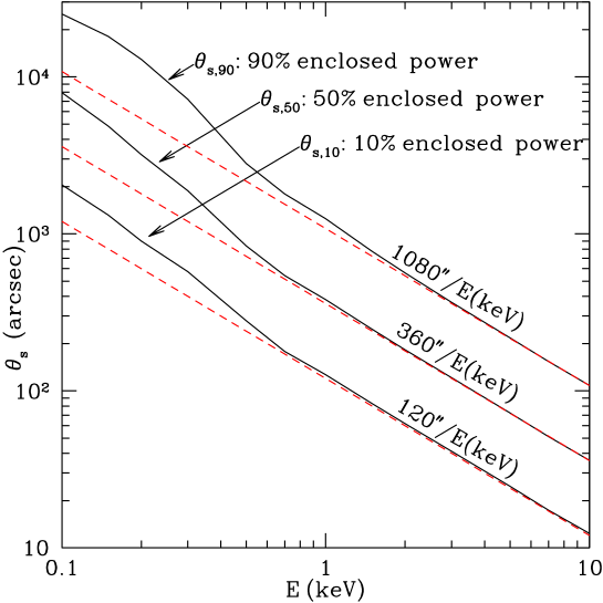
Figure 9: Median scattering angle $\theta_{s,50}$ as a function of energy for the WD01 grain model. Also shown are scattering angles $\theta_{s,10}$ and $\theta_{s,90}$ for 10% and 90% enclosed power. Broken lines show asymptotic behavior for $E\gtrsim 1\,{\rm keV}$.

For $E\gtrsim 0.5\,{\rm keV}$, the median scattering angle for the WD01 dust mixture can be approximated by

$$\theta_{s,50}\approx 360\arcsec\left(\frac{\,{\rm keV}}{E}\right)~{}~{}~{}.$$ (9)

The median scattering angle for a circular aperture of diameter $d$ is $0.53\lambda/d$ (Born & Wolf 1999), so equation (9) corresponds to the median scattering angle for an aperture of radius $0.19\micron$, consistent with the size of the grains which dominate the visual extinction and polarization of starlight, account for most of the interstellar grain mass, and are expected to dominate the X-ray scattering. The smaller grains, while more numerous, make only a minor contribution to scattering at $E\gtrsim 0.5\,{\rm keV}$. Note that at lower energies, the median scattering angle rises above the approximation (9), due in part to the increasing importance of smaller grains (which contribute most of the geometric cross section of the grain population) at these energies.

For this dust model, the differential scattering cross section can be approximated by the simple analytic form

$$\frac{d\sigma}{d\Omega}\approx\frac{\sigma_{\rm sca}}{\pi\theta_{s,50}^{2}}\frac{1}{\left[1+(\theta/\theta_{s,50})^{2}\right]^{2}}~{}~{}~{},$$ (10)

with the total cross section for scattering angles $<\theta$

$$\sigma_{\rm sca}(<\theta)=\sigma_{\rm sca}\frac{(\theta/\theta_{s,50})^{2}}{1+(\theta/\theta_{s,50})^{2}}~{}~{}~{}.$$ (11)

Eq. (11) reproduces the empirical result that $\theta_{s,10}=\theta_{s,50}/3$, and $\theta_{s,90}=3\theta_{s,50}$. The approximation (10) is plotted in Fig. 8 for $E=1.0$ and 5.0  keV, showing that it does indeed provide a good fit.

4 X-Ray Scattering Halos: Models

4.1 Models

For a point source at distance $D$, scattering by dust on the sightline a distance $r=xD$ from the observer produces a scattered halo around the point source (see, e.g., Draine & Tan 2003) with the halo angle $\theta_{h}$ related to the scattering angle $\theta_{s}$ through

$$\theta_{h}\approx(1-x)\theta_{s}~{}~{}~{}.$$ (12)

Let $N_{\rm halo}$ be the total flux of singly-scattered photons, and $N_{\rm halo}(<\theta_{h})$ be the flux of photons at halo angles $<\theta_{h}$. Define the fraction of halo photons interior to $\theta_{h}$:

$$g(\theta_{h})\equiv\frac{N_{\rm halo}(<\theta_{h})}{N_{\rm halo}}~{}~{}~{}.$$ (13)

If the dust density is assumed to be plane-parallel perpendicular to the sightline, then for the small-angle scattering appropriate to X-ray energies, the scattering halo is given by

$$g(\theta_{h})\equiv\int_{0}^{1}dx~{}\tilde{\rho}(x)\frac{\sigma_{\rm sca}(<\theta_{h}/(1-x))}{\sigma_{\rm sca}}~{}~{}~{},$$ (14)

where the dimensionless dust density

$$\tilde{\rho}(x)\equiv\frac{\rho(xD)}{\int_{0}^{1}\rho(xD)dx}~{}~{}~{},$$ (15)

where $\rho(r)$ is the dust density along the sightline at distance $r$ from the observer.

Because the differential scattering cross section for the WD01 dust mixture can be approximated by eq. (10,11), we have

$$g(\theta_{h})\approx\int_{0}^{1}\tilde{\rho}(x)\left[1+(1-x)^{2}(\theta_{s,50}/\theta_{h})^{2}\right]^{-1}~{}~{}~{}.$$ (16)

If the scattering is by a single sheet of dust at distance $x_{d}D$, then $\tilde{\rho}(x)=\delta(x-x_{d})$ and

$$g(\theta_{h})\approx\frac{(\theta_{h}/\theta_{h,50})^{2}}{1+(\theta_{h}/\theta_{h,50})^{2}}~{}~{}~{},~{}~{}~{}\theta_{h,50}=(1-x_{d})\theta_{s,50}~{}~{}~{}.$$ (17)

For a uniform dust density gradient (with $\beta=0$ corresponding to uniformly-distributed dust)

$$\tilde{\rho}(x)=(1-\beta)+2\beta x~{}~{}~{}~{}~{}(-1\leq\beta\leq 1)~{}~{}~{},$$ (18)

eq. (14) can be integrated to obtain

$$g(\theta_{h})=(1+\beta)\frac{\theta_{h}}{\theta_{s,50}}\arctan(\theta_{s,50}/\theta_{h})-\beta\left(\frac{\theta_{h}}{\theta_{s,50}}\right)^{2}\ln\left[1+(\theta_{s,50}/\theta_{h})^{2}\right]~{}~{}~{};$$ (19)

$g(\theta_{h})$ is plotted in Fig. 10 for 5 cases: $\beta=-1$ (1/4 of the dust between $x=0.5$ and 1); $\beta=-.5$ (3/8 of the dust between $x=0.5$ and 1); $\beta=0$ (uniform dust); $\beta=0.5$ (5/8 of the dust between $x=0.5$ and 1); $\beta=1$ (3/4 of the dust between $x=0.5$ and 1). Also plotted is the case where the dust is all at $x\ll 1$, with $\theta_{h}=\theta_{s}$. For the above dust distributions, Table 2 gives the halo angles $\theta_{h,10}$, $\theta_{h,50}$, $\theta_{h,90}$ enclosing 10%, 50%, and 90% of the halo power for single-scattering.

Table 2: Halo Structure Parameters for WD01 Dust

	dust density distribution
	$\beta=-1$	$\beta=-0.5$	uniform	$\beta=0.5$	$\beta=1$
$\theta_{h,10}/\theta_{s,50}$	0.1663	0.1032	.0664	.0467	.0353
$\theta_{h,50}/\theta_{s,50}$	0.631	0.530	0.429	0.337	0.262
$\theta_{h,90}/\theta_{s,50}$	2.084	1.882	1.660	1.413	1.139
$\theta_{h,10}\times(E/\,{\rm keV})$	$59.9\arcsec$	$37.2\arcsec$	$23.9\arcsec$	$16.8\arcsec$	$12.7\arcsec$
$\theta_{h,50}\times(E/\,{\rm keV})$	$227\arcsec$	$191\arcsec$	$154\arcsec$	$121\arcsec$	$94.3\arcsec$
$\theta_{h,90}\times(E/\,{\rm keV})$	$750\arcsec$	$678\arcsec$	$598\arcsec$	$509\arcsec$	$410\arcsec$

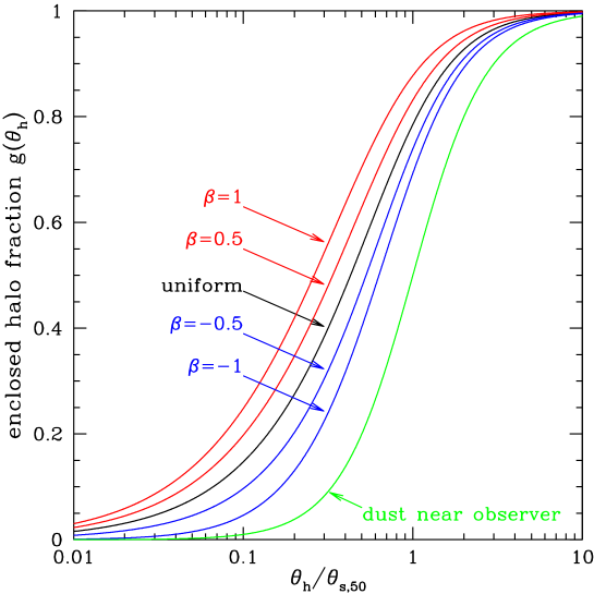
Figure 10: Fraction of the single-scattering halo falling within halo angle $\theta_{h}$, as a function of $\theta_{h}/\theta_{s,50}$, where $\theta_{s,50}$ is the median scattering angle.

5 X-Ray Scattering Halos: Observations

The total cross section for X-ray scattering can be measured by imaging the scattered X-ray halo. The flux of scattered photons, $N_{\rm halo}$, is related to the flux in the point-source component, $N_{\rm ptsrc}$, by $N_{\rm ptsrc}=(N_{\rm ptsrc}+N_{\rm halo})\exp(-\tau_{\rm sca})$, so

$$\tau_{\rm sca}=\ln(1+N_{\rm halo}/N_{\rm ptsrc})=-\ln\left(1-f_{\rm halo}\right)~{}~{}~{},$$ (20)

$$f_{\rm halo}\equiv\frac{N_{\rm halo}}{N_{\rm halo}+N_{\rm ptsrc}}~{}~{}~{};$$ (21)

eq. (20) is valid even when multiple scattering takes place. Absorption (by dust or gas) has a negligible effect on $N_{\rm halo}/N_{\rm ptsrc}$, because unscattered and scattered photons are affected essentially equally. Estimation of $\tau_{\rm sca}$ from (20) requires determination of the flux of scattered photons $N_{\rm halo}$ integrated over all halo angles. If the halo flux is measured only for halo angles $\theta_{1}<\theta_{h}<\theta_{2}$, the total halo flux can be estimated from

$$N_{\rm halo}=\frac{N_{\rm halo}(\theta_{1}<\theta_{h}<\theta_{2})}{g(\theta_{2})-g(\theta_{1})}~{}~{}~{};$$ (22)

the function $g(\theta_{h})$ depends, of course, on assumptions concerning both the grain model and the distribution of dust along the sightline.

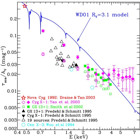
Figure 11: Scattering optical depth $\tau_{\rm sca}$ per unit visual extinction $A_{V}$ as calculated for the WD01 model (solid line) and as estimated from various observations (see text). Chandra imaging of GX 13+1 at $50\arcsec<\theta_{s}<600\arcsec$ (Smith, Edgar, & Shafer 2002) has been corrected for photons interior to $50\arcsec$ assuming uniformly distributed dust (open squares) or dust with density proportional to distance (filled squares). Chandra observations of Cyg X-1 at $\theta_{s}<120\arcsec$ (Yao et al. 2003) are uncorrected for photons beyond $120\arcsec$ (open diamonds) or corrected assuming uniform dust (filled diamonds). See text.

5.1 Cen X-3

Woo et al. (1994) used the ASCA X-ray observatory to measure the X-ray halo toward the massive X-ray binary Cen X-3 ($A_{V}\approx 4.3$) as a function of orbital phase, at 1.5 and $2.5\,{\rm keV}$. Their results for $\tau_{\rm sca}/A_{V}$ are shown in Figure 11. Also shown is the ratio $\tau_{\rm sca}/A_{V}$ estimated for the WD01 grain model. Woo et al.’s values of $\tau_{\rm sca}/A_{V}$ at 1.5 and 2.5 keV are a factor $\sim$3.5 below the prediction of the WD01 grain model. Can we understand this?

At 1.5 keV, the ASCA point spread function was such that even when the point source component was at a minimum, the halo intensity exceeded the point source intensity only for $\theta_{h}>200\arcsec$; when the point source was at maximum the halo intensity exceeded the point source intensity only for $\theta_{h}\gtrsim 450\arcsec$. For uniformly-distributed dust and $E=1.5\,{\rm keV}$, we expect a median halo angle $\theta_{h,m}\approx 100\arcsec$ (see Table 2); it is therefore clear that the ASCA observations were insensitive to most of the scattered photons. It therefore seems plausible that the scattered flux may have been underestimated by factors of 2-4 due to the dominance of the point source profile at halo angles $\theta\lesssim 200-400\arcsec$. The determination of $\tau_{\rm sca}/A_{V}$ by Woo et al. should be treated as a lower bound rather than a measurement.

5.2 ROSAT Observations

ROSAT observed both unscattered and scattered X-rays from Nova Cygni 1992 at a number of epochs (Krautter et al. 1996). The most recent reanalysis of the ROSAT data found $\tau_{\rm sca}=0.211\pm 0.006$ at the median photon energy $\sim$480 eV (Draine & Tan 2003). Adopting $E(B-V)=0.19$ estimated from observations of H$\alpha$/H$\beta$ (Barger et al. 1993; Mathis et al. 1995), we obtain $\tau_{\rm sca}/A_{V}=0.36$. As seen in Figure 11, this value is in excellent agreement with the WD01 grain model. Draine & Tan have also carried out detailed modelling, and conclude that the observed X-ray halo profiles at 9 different epochs are in good agreement with the WD01 dust model.

Predehl & Schmitt (1995, hereafter PS95) used ROSAT to estimate $f_{\rm halo}$ for Cyg X-1, GX 13+1, and 19 other galactic sources for which $A_{V}$ was also available. In each case, PS95 have fitted the observations with the ROSAT psf plus a theoretical dust model, and used this to estimate the total number of scattered photons. Figure 11 shows the resulting $\tau_{\rm sca}/A_{V}$ versus the average photon energy for each source. The estimates of $\tau_{\rm sca}/A_{V}$ inferred from the PS95 observations are generally a factor $\sim 2-4$ below the WD01 grain model. If the PS95 values of $f_{\rm halo}$ are accurate, this would indicate a serious problem with the WD01 grain model.

However, for the 21 sources, the halo angle at which the intensities of the fitted halo and psf were equal was $70\arcsec$ or larger; for 50% of the sources this angle was $130\arcsec$ or larger. At a typical energy of $\sim$1.2 keV, the median scattering angle is $\theta_{h,50}\approx 130\arcsec$ for uniformly-distributed dust (see Table 2). Estimates of $f_{\rm halo}$ therefore rely heavily on the dust model to separate the halo from the point source at small halo angles. The modelling by PS95 employed power-law grain size distributions $dn/da\propto a^{-q}$ for $a<a_{\rm max}$. For the 21 sources, the median $q$ value was 4.0 and the median value of $a_{\rm max}$ was $0.18\micron$. Power-law grain size distributions with $q\approx 3.5$ and $a_{\rm max}\approx 0.25\micron$ (Mathis, Rumpl, & Nordsieck 1977; Draine & Lee 1984) provide a good fit to the interstellar extinction, but the size distributions adopted by PS95 – with generally steeper power laws and smaller values of $a_{\rm max}$ – had insufficient mass in large grains and do not provide a good fit to the extinction law. The scattering at small halo angles is dominated by the larger grains, so the PS95 model-fitting may have systematically underestimated the actual halo intensity at small halo angles.

Given likely uncertainties in the psf and the model-fitting, it seems likely that the PS95 values of $\tau_{\rm sca}/A_{V}$ are systematically low, perhaps by factors as large as 2-4. We now examine two particular sightlines.

5.3 GX 13+1

GX 13+1 is a low-mass X-ray binary system at $l=13.5^{\circ}$, $b=0.10^{\circ}$, and an estimated distance $D\approx 7\,{\rm kpc}$, corresponding to a distance above the plane $D\sin b\approx 12\,{\rm pc}$. Garcia et al. (1992) estimated $A_{V}\lesssim 14.4$. X-ray spectroscopy gives $N_{\rm H}=2.9\pm 0.1\times 10^{22}\,{\rm cm}^{-2}$ (Ueda et al. 2001), corresponding to $A_{V}=15.5$ for the standard conversion $N_{\rm H}/A_{V}=1.87\times 10^{21}\,{\rm cm}^{-2}$ (Bohlin, Savage, & Drake 1978). We adopt $A_{V}=14$. The mean photon energy for the ROSAT observations is $E=1.69\,{\rm keV}$ (PS95).

PS95 find a halo fraction $f_{\rm halo}=0.335$ for GX 13+1, but (as discussed above) this may be an underestimate:

• For GX 13+1, PS95 estimate that the halo and psf have equal intensities at $\sim$75″ (see their Fig. 10). For uniformly-distributed dust and $E=1.69\,{\rm keV}$, the median halo angle $\theta_{h,50}\approx 91\arcsec$, but on this sightline the dust density may be enhanced closer to the source, leading to a reduction in $\theta_{h,50}$; for a linear gradient with $\beta=1$, $\theta_{h,50}\approx 58\arcsec$. Thus it appears possible that $\gtrsim 50\%$ of the scattered photons may have been misattributed to the psf.

• For GX 13+1, PS95 used a dust model with $dn/da\propto a^{-3.8}$ and $a_{\rm max}=0.18\micron$; as discussed above, this underestimates the abundances of $a\gtrsim 0.1\micron$ grains, and therefore underestimates the contribution of scattering at small halo angles.

It therefore appears that PS95 could have underestimated $N_{\rm halo}$. While difficult to quantify, it seems possible that the true value of $f_{\rm halo}$ might be as large as 0.65 (the value predicted by the WD01 grain model for $E=1.69\,{\rm keV}$ and $A_{V}=14$).

The X-ray halo around GX 13+1 has recently been observed by the Chandra X-ray telescope (Smith, Edgar, & Schafer 2002) at energies between 2.1 and $3.9\,{\rm keV}$, with energy resolution $\sim 0.2\,{\rm keV}$. Phenomena referred to as “pileup” and “grade migration” in the detection system affect the Chandra ACIS images as far as $50\arcsec$ from the source. Smith et al. also discuss the current uncertainties concerning the Chandra psf at angles $>50\arcsec$. Using a preliminary psf based on observations of Her X-1, they estimate what they refer to as “total observed halo fraction” $I(E)$ by integrating the psf-subtracted and background-subtracted count rates from $50\arcsec$ to $600\arcsec$, and dividing by the estimated psf count rate in the absence of saturation effects. Thus

$$I(E)=\frac{(1-e^{-\tau_{\rm sca}})[g(600\arcsec)-g(50\arcsec)]}{e^{-\tau_{\rm sca}}}~{}~{}~{}.$$ (23)

If we assume a model for the dust distribution, we can use $g(\theta_{h})$ to obtain

$$\tau_{\rm sca}=\ln\left[1+\frac{I}{[g(600\arcsec)-g(50\arcsec)]}\right]~{}~{}~{},$$ (24)

where for a uniform gradient $g(\theta_{h})$ is given by eq. (19). In Figure 11 we show the values of $\tau_{\rm sca}/A_{V}$ obtained from the observed $I$, with $g(\theta_{h})$ calculated for the WD01 grain model assuming (a) uniformly-distributed dust ($\beta=0$) and (b) dust with a density gradient $\beta=1$. Given the location of this source, we expect the dust density to be increasing toward the source, so the $\beta=1$ model is reasonable. For $\beta=1$, the inferred $\tau_{\rm sca}/A_{V}$ is a factor $\sim$1.5 below the WD01 model for 2.4–3.4 keV, and a factor 1.1–1.3 below the WD01 model at 3.4–4.0 keV. These observations suggest that the WD01 model may overestimate $\tau_{\rm sca}/A_{V}$, although it should be kept in mind that these results required substantial corrections for unobserved halo interior to $50\arcsec$.

The best way to use the information in the oberved scattered halo is to try to reproduce the observed radial profile of the scattered halo using a dust model, and Smith et al. tested various grain models in this way. For dust distributed uniformly between source and observer, for the WD01 grain model they find a best-fit gas column $N_{\rm H}=1.65\times 10^{22}\,{\rm cm}^{-2}$, significantly smaller than the value $2.9\pm 0.1\times 10^{22}\,{\rm cm}^{-2}$ estimated from ASCA observations (Ueda et al. 2001). Note, of course, that additional dust could be located at $x>0.75$ without appreciably affecting the observed $I(\theta_{h}>50\arcsec)$, since the additional halo contribution would be mainly below the $50\arcsec$ lower cutoff.

5.4 Cygnus X-1

Cygnus X-1 consists of an O star primary with a black hole companion (see Tanaka & Lewin 1995), located at $l=71.33^{\circ}$, $b=3.07^{\circ}$, and an estimated distance $D=2.5\pm 0.4\,{\rm kpc}$ (Bregman et al. 1973; Ninkov et al. 1986), placing it at a height $D\sin b\approx 130\pm 20\,{\rm pc}$ above the plane. The O9.7 Iab primary is reddened by $E(B-V)=1.12$ (Bregman et al. 1973), corresponding to $A_{V}=3.5$; this is consistent with $N_{\rm H}=6.2\times 10^{21}\,{\rm cm}^{-2}$ from X-ray absorption spectroscopy (Schulz et al. 2002). Based on studies of reddening vs. distance for stars within $50\arcmin$ of Cyg X-1 (Bregman et al. 1973; Margon et al. 1973) it appears that the dust is distributed approximately uniformly along the sightline.

PS95 observed Cygnus X-1 with ROSAT, and found $f_{\rm halo}=0.116$ at 1.2 keV. The psf and scattered halo intensity were estimated to be equal at $\theta\approx 110\arcsec$. The PS95 result $\tau_{\rm sca}/A_{V}=.037\,{\rm mag}^{-1}$ at $1.2\,{\rm keV}$ is a factor 3 below the WD01 model (see Fig. 11).

Yao et al. have recently used Chandra observations of Cygnus X-1 to infer the scattered halo, using a technique designed to minimize the effects of “pileup”, allowing the excellent angular resolution of Chandra to be used to observe at small halo angles. Yao et al. neglected halo angles $\theta>120\arcsec$, but were able to measure the halo as close as $1\arcsec$ from the point source. Their fractional halo intensity ${\rm FHI}$ is the ratio of the halo counts interior to 120$\arcsec$ divided by the counts from the psf plus the halo interior to 120$\arcsec$, and is related to $\tau_{\rm sca}$ by

$${\rm FHI}=\frac{(1-e^{-\tau_{\rm sca}})g(120\arcsec)}{e^{-\tau_{\rm sca}}+(1-e^{-\tau_{\rm sca}})g(120\arcsec)}~{}~{}~{}.$$ (25)

Yao et al. also report the radius $\theta_{*}$ containing 50% of the halo counts within $120\arcsec$ of the source, i.e., $g(\theta_{*})=0.5g(120\arcsec)$. In Figure 12 we show the variation of $\theta_{*}$ with $E$ calculated for: (1) uniform dust; (2) thin sheet at $x_{d}=0.7$; (3) thin sheet at $x_{d}=0.8$; (4) thin sheet at $x_{d}=0.9$. The single sheet models clearly do not reproduce the observations. The uniform dust model is in approximate overall agreement with the distribution of halo counts within 120$\arcsec$, although it does not reproduce the concentration of the halo at $E<3\,{\rm keV}$ found by Yao et al.

Figure 12: Radius $\theta_{*}$ enclosing 50% of the halo counts within $120\arcsec$ of the point source. Data points are observations of Cyg X-1 by Yao et al. (2003).

Adopting the uniform dust model, we can now use the WD01 model to correct for halo counts at $\theta_{h}>120\arcsec$: $\tau_{\rm sca}=\ln\{1+{\rm FHI}/[(1-{\rm FHI})g(120\arcsec)]\}$, with the results plotted in Fig. 11. At $E<2.5\,{\rm keV}$, where the estimated fractional uncertainties are smallest, the values of $\tau_{\rm sca}/A_{V}$ found from the Yao et al. results fall a factor $\sim 1.5-2$ below the predictions of the WD01 model. The reason for this is not apparent. Perhaps the WD01 model has overestimated $\tau_{\rm sca}/A_{V}$; alternatively, perhaps the background has been overestimated – background oversubtraction would be consistent with the surprising concentration of the halo seen at $E<2.5\,{\rm keV}$ in Fig. 12.

For 3–4$\,{\rm keV}$, the inferred values of $\tau_{\rm sca}/A_{V}$, and the measured halo half-light radii in Fig. 12, are consistent with the WD01 dust model. However, at $5-7\,{\rm keV}$ the values of $\tau_{\rm sca}/A_{V}$ measured by Yao et al. exceed the predictions of the WD01 model, although the error bars are now large. It is difficult to envision a dust model which could have such a large value of $\tau_{\rm sca}/A_{V}$ at these energies, so we suspect that the observations are affected by some systematic error – perhaps the wings of the Chandra psf at these energies may have been underestimated, or the novel method employed by Woo et al to reconstruct the radial profile may be prone to systematic errors which are not fully understood.

5.5 Discussion

We have reviewed a number of measurements of dust scattering halos, and compared the predictions of the WD01 grain model to the values of $\tau_{\rm sca}/A_{V}$ estimated from these observations. The results, shown in Fig. 11, are somewhat equivocal. Two studies (Woo et al. 1994; Predehl & Schmitt 1995) find values of $\tau_{\rm sca}/A_{V}$ much lower than expected for the WD01 dust model, but we give arguments why these observations might have underestimated $\tau_{\rm sca}$.

Draine & Tan (2003) have quantitatively modelled the X-ray halo around Nova Cygni 1992 (typical photon energy $\sim$0.48 keV) using the WD01 grain model. The halo intensity observed by ROSAT can be reproduced using a dust column density which agrees with the reddening inferred from the observed H$\alpha$/H$\beta$ intensity ratio.

Chandra observations of GX 13+1 by Smith et al. (2002), after correcting for missed halo counts using the constant dust gradient model with $\beta=1$, give $\tau_{\rm sca}/A_{V}$ within a factor $\sim$1.5 of the WD01 model at 2 keV, and in agreement at 3.5–4 keV. The corrections are somewhat sensitive to the (uncertain) dust density distribution for this case, since the halo intensity was not measured at $\theta_{h}<50\arcsec$.

The recent Chandra measurement of the halo around Cyg X-1 (Yao et al. 2003) implies values of $\tau_{\rm sca}/A_{V}$ which are a factor $\sim$1.5–2 smaller than expected for the WD01 model at $E<2.5\,{\rm keV}$. At 3–4 keV the Yao et al. results are in excellent agreement with the WD01 model in terms of both $\tau_{\rm sca}/A_{V}$ and the half-light radius of the halo. For 5–7 keV the values of $\tau_{\rm sca}/A_{V}$ found by Yao et al. exceed the WD01 model by factors of 2–3, although the estimated errors are also large.

Taken together, the Chandra observations of GX 13+1 (Smith et al. 2002) and of Cyg X-1 (Yao et al. 2003) suggest that the WD01 model may have overestimated $\tau_{\rm sca}/A_{V}$ by a factor $\sim$1.5 between 1 and 2.5 keV. However, the Yao et al observations of Cyg X-1 at 3–4 keV give both a halo concentration and $\tau_{\rm sca}/A_{V}$ in good agreement with the WD01 model, and the WD01 model is also consistent with the Nova Cygni observations at $\sim$0.5 keV (Draine & Tan 2003). At this time we can conclude only that the WD01 model appears to give $\tau_{\rm sca}/A_{V}$ in agreement with observations to within a factor $\sim$1.5, but the existing observations do not permit a more precise statement.

It is hoped that future observations by Chandra or XMM will be able to carry out high-signal-to-noise observations of X-ray scattering halos on sightlines where the dust distribution and reddening are well-determined. An optimal situation would be to use a source which is known to be distant compared to the dust doing the scattering, so that we can assume that $x\lesssim 0.2$ in eq. (12). An extragalactic X-ray point source (AGN or quasar) would be ideal for this purpose.

6 Summary

The following are the principal results of this work:

1. Dielectric functions for graphite and MgFeSiO₄ have been constructed which are continuous from submm to hard X-rays, obey the Kramers-Kronig relations, and satisfy the oscillator strength sum rule.

2. Absorption, scattering, and extinction have been calculated for the WD01 grain model at X-ray energies. The calculated absorption edge structure appears to be consistent with recent spectroscopy by the Chandra X-Ray Observatory, and can be further tested by future observations.

3. Differential scattering cross sections are presented for the Milky Way dust model at X-ray energies. These can be used for modelling X-ray scattering halos, and are available at http://www.astro.princeton.edu/$\sim$draine .

4. The median scattering angle $\theta_{s,50}(E)$ is given, as well as the scattering angles $\theta_{s,10}$ and $\theta_{s,90}$ for 10% and 90% enclosed power. These can be used to assess the sensitivity of imaging observations for determination of the flux of halo photons.

5. Simple analytic functions provide a good approximation to the differential scattering cross section for dust (eq. 10,11).

6. We provide analytic approximations to $g(\theta_{h})$, the fraction of the halo counts interior to $\theta_{h}$, for dust in a single sheet (eq. 17) and uniformly-distributed dust or dust with a density gradient (eq. 19).

7. The total scattering cross section calculated for the WD01 grain model is compared with observations of X-ray halos by ASCA, ROSAT, and Chandra (see Fig. 11). The results are somewhat equivocal, and in some cases depend on corrections which are sensitive to the spatial distribution of the dust. ROSAT observations of Nova Cygni 1992 at $\sim$0.5 keV (Draine & Tan 2003), and Chandra observations at 3–4 keV of Cyg X-1 (Yao et al. 2003) are in good agreement with the WD01 dust model, although the 2–3.4 keV observations of GX 13+1, and 1–3 keV observations of Cyg X-1, give $\tau_{\rm sca}/A_{V}$ about a factor $\sim$1.5 below the WD01 model. At this time it is possible to conclude from the observations that $\tau_{\rm sca}/A_{V}$ given by the WD01 model is accurate to within a factor $\sim$1.5, but a more precise statement is not possible.

8. Analysis of the angular structure of X-ray halos around Galactic sources will generally be compromised by uncertainties concerning the location of the dust responsible for the scattering. The ideal observation is to observe an extragalactic point source, in which case the scattering dust is all at $x\approx 0$. It is hoped that such observations will be carried out by Chandra or XMM for bright extragalactic sources located behind sufficient Galactic dust, thereby providing a definitive test of this and other dust models.

References

- Altarelli et al (1972) Altarelli, M., Dexter, D.L., Nussenzveig, H.M., & Smith, D.Y. 1972, Phys. Rev. B, 6, 4502
- Barger et al (1993) Barger, A.J., Gallagher, J.S. III, Bjorkman, K.S., Johansen, K.A., & Nordsieck, K.H. 1993, ApJ, 419, L85
- Bohlin et al (1978) Bohlin, R.C., Savage, B.D., & Drake, J.F. 1978, ApJ, 224, 132
- Boese (2000) Boese, F.G. 2000, A&AS, 141, 507
- Born & Wolf (1999) Born, M., & Wolf, E. 1999, Principles of Optics, 7th ed. (Cambridge: Cambridge Univ. Press) §8.5.2
- Bregman et al (1973) Bregman, J., Butler, D., Kemper, E, Koski, A., Kraft, R.P., & Stone, R.P.S. 1973, ApJ, 185, L117
- Djurisic & Li (1999) Djurisic, A., & Li, E.H. 1999, J. Appl. Phys., 85, 7404
- (8) Draine, B.T. 2003a, ARAA, 41, 241
- (9) Draine, B.T. 2003b, ApJ, submitted (Paper I).
- Draine & Lee (1984) Draine, B.T., & Lee, H.-M. 1984, ApJ, 468, 269 (DL84)
- Draine & Li (2001) Draine, B.T., & Li, A. 2001, ApJ, 551, 807
- Draine & Tan (2003) Draine, B.T., & Tan, J.C. 2003, ApJ, 594, 000 (Sept 1) [http://arxiv.org/abs/astroph/0208302]
- Garcia et al (1992) Garcia, M.R., Grindlay, J.E., Bailyn, C.D., Pipher, J.L., Shure, M.A., & Woodward, C.E. 1992, AJ, 103, 1325
- Garvie et al (2000) Garvie, L.A.J., Rez, P., Alvarez, J.R., Buseck, P.R., Craven, A.J., & Brydson, R. 2000, American Mineralogist, 85, 732
- Gordon et al (2003) Gordon, M.L., Tulumello, D., Cooper, G., Hitchcock, A.P., Glatzel, P., Mullins, O.C., Cramer, S.P., & Bergmann, U. 2003, submitted to J. Phys Chem B
- Hayakawa (1970) Hayakawa, S. 1970, Prog. Theor. Phys., 43, 1224
- Henderson et al (1995) Henderson, C.M.B, Cressey, G., & Redfern, S.A.T. 1995, Radiat. Phys. Chem. 45, 459
- Kim & Martin (1995) Kim, S.-H., & Martin, P.G. 1995, ApJ, 442, 172
- Krautter et al (1996) Krautter, J., Ögelman, H., Starrfield, S., Wichmann, R., & Pfeffermann, E. 1996, ApJ, 456, 788
- Landau & Lifshitz (1960) Landau, L.D., & Lifshitz, E.M. 1960, Electrodynamics of Continuous Media (New York: Pergamon) §62.
- Laor & Draine (1993) Laor, A., & Draine, B.T. 1993, ApJ, 402, 441
- Li et al (1995) Li, D., Bancroft, G.M., Fleet, M.E., & Feng, X.H. 1995, Phys. Chem. Minerals, 22, 115
- Li & Draine (2001) Li, A., & Draine, B.T. 2001, ApJ, 554, 778
- Li & Draine (2002) Li, A., & Draine, B.T. 2002, ApJ, 572, 232
- Marcelli et al (1985) Marcelli, A, Davoli, I, Bianconi, A, Garcia, J., Gargano, A, et al. 1985, J. de Physique, 46, 107
- Margon et al (1973) Margon, B., Bowyer, S., & Stone, R.P.S. 1973, ApJ, 185, L113
- Martin (1970) Martin, P.G. 1970, MNRAS, 149, 221
- Mathis et al (1995) Mathis, J.S., Cohen, D., Finley, J.P., & Krautter, J. 1995, ApJ, 449, 320
- Mathis et al (1977) Mathis, J.S., Rumpl, W., & Nordsieck, K.H. 1977, ApJ, 217, 425
- McLaughlin & Kirby (1998) McLaughlin, B.M., & Kirby, K,P. 1998, J. Phys. B, 31, 4991
- Ninkov et al (1986) Ninkov, Z, Walker, G.A.H, & Yang, S. 1986, ApJ, 321, 425
- Overbeck (1965) Overbeck, J.W. 1965, ApJ, 141, 864
- Paerels et al (2001) Paerels, F., Brinkman, A.C., van der Meer, R.L.J., Kaastra, J.S., Kuulers, E., Boggende, A.J.F. den, Predehl, P., et al. 2001, ApJ, 546, 338
- Predehl & Schmitt (1995) Predehl, P., & Schmitt, J.H.M.M. 1995, A&A, 293, 889 (PS95)
- Schulz et al (2002) Schulz, N.S., Cui, W., Canizares, C.R., Marshall, H.L., Lee, J.C., Miller, J.M., & Lewin, W.H.G. 2002, ApJ, 565, 1141
- Sharp et al (1996) Sharp, T., Wu, Z., Seifert, F., Poe, B., Doerr, M., & Paris, E. 1996, Phys. Chem. Minerals, 23, 17
- Shimada et al (2000) Shimada, H., Imamura, M., Matsubayashi, N., Saito, T., Tanaka, T., Hayakawa, T., & Kure, S. 2000, Topics in Catalysis, 10, 265
- Smith et al. (2002) Smith, R.K., Edgar, R.J., & Shafer, R.A. 2002, ApJ, 581, 562
- Stolte et al (1997) Stolte, W.C., Samson, J.A.R., Hemmers, O., Hansen, D, Whitfield, S.B., & Lindle, D.W. 1997, J. Phys. B, 30, 4489
- Takei et al. (2002) Takei, Y., Fujimoto, R., Mitsuda, K., & Onaka, T. 2002, ApJ, 581, 307
- Tanaka & Lewin (1995) Tanaka, Y., & Lewin, W.H.G. 1995, in X-Ray Binaries, ed. W.H.G. Lewin, J. van Paradijs, & E.P.J. van den Heuvel (Cambridge: Cambridge Univ. Press), 126
- Ueda et al (2002) Ueda, Y., Asai, K., Yamaoka, K., Dotani, T., & Inoue, H. 2001, ApJ, 556, L87
- van Aken & Liebscher (2002) van Aken, P.A., & Liebscher, B. 2002, Phys. Chem. Minerals, 29, 188
- van Aken et al. (1998) van Aken, P.A., Liebscher, B., & Styrsa, V.J. 1998, Phys. Chem. Minerals, 25, 323
- van de Hulst (1957) van de Hulst, H.C. 1957, Light Scattering by Small Particles (New York: Wiley)
- Verner (1996) Verner, D.A. 1996, http://www.pa.uky.edu/verner/photo.html
- Verner et al (1996) Verner, D.A., Ferland, G.J., Korista, K.T., & Yakovlev, D.G. 1996, ApJ, 464, 487
- Verner & Yakovlev (1995) Verner, D.A., & Yakovlev, D.G. 1995, A&A Suppl., 109, 125
- Weingartner & Draine (2001) Weingartner, J.C., & Draine, B.T. 2001, ApJ, 548, 296 (WD01)
- Wiscombe (1980) Wiscombe, W.J. 1980, Appl. Opt., 19, 1505
-
Wiscombe (1996)
Wiscombe, W.J. 1996,
NCAR Technical Note NCAR/TN-140+STR,
ftp://climate.gsfc/nasa.gov/pub/wiscombe/SingleScatt/Homogen_Sphere/Exact_Mie/ NCARMieReport.pdf - Woo (1995) Woo, J.W. 1995, ApJ, 447, L129
- Woo et al (1994) Woo, J.W., Clark, G.C., Day, C.S.R., Nagase, F., & Takeshima, T. 1994, ApJ, 436, L5
- Wu et al (1996) Wu, Z., Seifert, F., Poe, B., & Sharp, T. 1996, J. Phys: Condensed Matter, 8, 3323.
- Yao et al (2003) Yao, Y., Zhang, S.N., Zhang, X.L., & Feng, Y.X. 2003, ApJ, accepted; astro-ph/0303149v2