Resonant Trapping of Planetesimals by Planet Migration: Debris Disk Clumps and Vega’s Similarity to the Solar System

Abstract

This paper describes a model which can explain the observed clumpy structures of debris disks. Clumps arise because after a planetary system forms its planets migrate due to angular momentum exchange with the remaining planetesimals. Outward migration of the outermost planet traps planetesimals outside its orbit into its resonances and resonant forces cause azimuthal structure in their distribution. The model is based on numerical simulations of planets of different masses, $M_{pl}$, migrating at different rates, $\dot{a}_{pl}$, through a dynamically cold ($e<0.01$) planetesimal disk initially at a semimajor axis $a$. Trapping probabilities and the resulting azimuthal structures are presented for a planet’s 2:1, 5:3, 3:2, and 4:3 resonances. Seven possible dynamical structures are identified from migrations defined by $\mu=M_{pl}/M_{\star}$ and $\theta=\dot{a}_{pl}\sqrt{a/M_{\star}}$. Application of this model to the 850$\mu$m image of Vega’s disk shows its two clumps of unequal brightness can be explained by the migration of a Neptune-mass planet from 40 to 65AU over 56Myr; tight constraints are set on possible ranges of these parameters. The clumps are caused by planetesimals in the 3:2 and 2:1 resonances; the asymmetry arises because of the overabundance of planetesimals in the 2:1(u) over the 2:1(l) resonance. The similarity of this migration to that proposed for our own Neptune hints that Vega’s planetary system may be much more akin to the solar system than previously thought. Predictions are made which would substantiate this model, such as the orbital motion of the clumpy pattern, the location of the planet, and the presence of lower level clumps.

1 Introduction

The discovery of disks of dust around main sequence stars showed that some grain growth must have occurred in these systems, since this dust is short-lived and so must be continually replenished (e.g., Backman & Paresce 1993); the dust is thought to originate in a collisional cascade that starts with planetesimals a few km in size (Wyatt & Dent 2002). Thus the lack of warm dust in the inner $\sim 30$ AU of these systems implies a relative paucity of planetesimals in these regions (Laureijs et al. 2002). This would naturally be explained if the planetesimals here grew large enough for their gravitational perturbations to clear these regions of any remaining debris, i.e., if they grew to $\gg 1000$ km sized planets (Kenyon & Bromley 2002). While the presence of such planets is still questionable, it is widely believed that these debris disk systems are solar system analogs, and that the dust that is observed is produced by the destruction of analog Kuiper belts (Wyatt et al. 2003).

The most positive indication that debris disk systems harbor planets comes from the morphology of the dust disks. All of the disks which have been imaged exhibit clumps and asymmetries which have been interpreted as perturbations from a planetary system: e.g., a brightness asymmetry in the HR4796 disk (Telesco et al. 2000) can be explained by the secular gravitational perturbations of a planet on an eccentric orbit (Wyatt et al. 1999); clumps observed in the $\epsilon$ Eridani, Vega and Fomalhaut disks (Holland et al. 1998; Greaves et al. 1998; Wilner et al. 2002; Holland et al. 2003) may be indicative of dust trapped in mean motion resonance with a planet in these systems (Ozernoy et al. 2000; Wyatt & Dent 2002; Quillen & Thorndike 2002; Kuchner & Holman 2003); and a warp in the $\beta$ Pictoris disk (Heap et al. 2000) may be caused by the perturbations of a planet on an inclined orbit (Augereau et al. 2001).

This paper focuses on the possibility that clumps in debris disks are caused by dust trapped in planetary resonances. Simple geometrical arguments show how material that is in such resonances is not evenly distributed in azimuth about the star it is orbiting (e.g., Murray & Dermott 1999; see §4), and this observation has been exploited by several authors to use debris disk clumps to infer the presence of planets. In the studies currently in the literature, dust is trapped into planetary resonances when it encounters these resonances while spiraling in towards the star due to P-R drag, much in the same way that dust originating in the asteroid belt becomes trapped in resonance with the Earth (Dermott et al. 1994), and dust originating in the Kuiper belt might become trapped in resonance with Neptune (Moro-Martín & Malhotra 2002). However, Wyatt et al. (1999) showed that P-R drag is not important for dust in the bright debris disks that are currently known, since these are much denser than the zodiacal cloud or the putative Kuiper belt dust cloud. This means that debris disk dust is destroyed in mutual collisions much faster than the P-R drag timescale until it is small enough to be blown out of the system by radiation pressure.

Another reason why dust may be trapped in planetary resonances is evident by comparison with the solar system. About one third of known Kuiper belt objects (hereafter KBOs), including Pluto, are trapped in 3:2 resonance with Neptune (Jewitt 1999). More recently KBOs have also been found in Neptune’s other resonances, including the 1:1, 4:3, 7:4, 2:1, and 5:2 resonances Chiang et al. (2003). These planetesimals are thought to have become trapped in these resonances when Neptune’s orbit expanded in the early history of the solar system (Malhotra 1995). In this scenario, the orbital expansion arises from angular momentum exchange resulting from the scattering by Neptune of the residual planetesimal disk left over at the end of planet formation; the current orbital distribution seen in the Kuiper belt can be explained by the migration of Neptune from 23-30 AU over a period of 50 Myr (Hahn & Malhotra 1999). While this model does not completely describe the KBO distribution, it turns out that some of its puzzling features, such as the high inclination population of the classical KBOs (i.e., those not trapped in resonance with Neptune), can now be accounted for with more detailed models of the migration (Gomes 2003). Besides, the success with which it explains the orbital distribution of the resonant KBOs means that the migration of Neptune is almost certain to have played a role in the formation of the Kuiper belt. Furthermore, models of the formation of such massive planets in the absence of the substantial accretion of gaseous material predicts such migration (Fernández & Ip 1984). Thus if planets did form in the inner regions of debris disk systems, some fraction of the parent planetesimals from which the dust originates is expected to be trapped in resonance with the outermost planet of that system.

Current studies of planet migration and the consequent resonant trapping deal with the migration of Neptune and its effect on the Kuiper belt (Malhotra 1995; Hahn & Malhotra 1999; Zhou et al. 2002; Chiang & Jordan 2002). This study is the first in a series which aims to determine the effect of planet migration in extrasolar systems. In such systems, planets of different mass may have formed at different distances from different mass stars; they also may have migrated at different speeds. This paper explores the effect of planet migration on a planetesimal disk, while the details of how the planet achieves that migration and of the dust distribution resulting from the destruction of these planetesimals are left for future studies in the series.

The layout of the paper is as follows. The numerical model of planet migration is described in §2 and in §3 this is used to calculate the probability of capture of planetesimals into different resonances for given migration scenarios. §4 shows how the geometry of resonant planetesimal orbits causes their distribution to be clumpy and parameters defining this clumpiness are derived from the numerical simulations. In §5 I show how these results can be applied to the structure of debris disks using the specific example of the structure observed around Vega to set constraints on the mass and migration history of planets in this system. The conclusions are given in §6.

2 Numerical Model

The dynamical evolution of a system comprised of 200 planetesimals and 1 planet was followed using the RADAU fifteenth order integrator program (Everhart 1985). This integration scheme is self-starting in that the time steps of each sequence are variable and are chosen by the integrator based on the results of the previous sequence; substeps within each sequence are taken at Gauss-Radau spacings.

In these integrations all bodies are assumed to orbit a star of mass $M_{\star}$. The planet has a mass of $M_{pl}$ while the planetesimals are assumed to be massless, i.e., they do not affect the evolution of the planet’s orbit though they are affected by it. At the start of the integration, the planetesimals are assumed to have eccentricities, $e$, chosen randomly from the range 0 to 0.01. Their inclinations, $I$, were chosen randomly from the range 0 to $0.57^{\circ}=0.01$ rad, and their arguments of periastron, $\tilde{\omega}$, longitudes of ascending node, $\Omega$, and longitudes, $\lambda$, were each chosen randomly from the range 0 to $360^{\circ}$. The planet was assumed to have all of these orbital parameters set to zero at the start of the integration; i.e., the planet starts on a circular orbit in the mid-plane of the planetesimal disk. The initial semimajor axes of the planetesimals, $a$, and that of the planet, $a_{pl}$, were set according to the integration being performed.

Planet migration was simulated by the addition of a force acting in the direction of orbital motion of the planet. The prescription for the force used in this paper has as its input the variable $\dot{a}_{var}$ and results in an acceleration of:

$$\dot{v}=0.5\dot{a}_{var}\sqrt{GM_{\star}/a^{3}}.$$ (1)

Since the work done by this force results in a change in orbital energy (see e.g., section 2.9 of Murray & Dermott 1999), this causes a change in the planet’s semimajor axis of $\dot{a}=2\dot{v}\sqrt{a^{3}/GM_{\star}}=\dot{a}_{var}$; i.e., the force defined by $\dot{v}$ results in a constant rate of change in the planet’s semimajor axis. The planet maintains its circular orbit ($e_{pl}=0$) in the midplane of the disk ($I_{pl}=0$).

The integrator itself has been extensively tested, and the addition of planet migration was tested by repeating simulation Ia of Chiang & Jordan (2002). The resulting final distribution of eccentricities, inclinations and semimajor axes of planetesimals was qualitatively the same as that depicted in their figure 3.

3 Resonant Capture Probabilities

Planetary resonances are locations at which planetesimals orbit an integer $p$ number of times for every integer $p+q$ times that the planet orbits the star. Kepler’s third law shows that resonances occur at semimajor axes of:

$$a_{p+q:p}=a_{pl}\left(\frac{p+q}{p}\right)^{2/3}.$$ (2)

If the planet is migrating at a rate $\dot{a}_{pl}$, these resonances only remain in the vicinity of planetesimals at a given semimajor axis for a short time. However, while close to a planetary resonance, a planetesimal receives periodic kicks to its orbit from the gravitational perturbations of the planet. These can impart angular momentum to the planetesimal so that its semimajor axis increases in such a way that the planetesimal is always orbiting at the location of the resonance; such a planetesimal is said to be trapped in the planet’s resonance. The resonant forces causing this trapping are discussed in greater detail in §4.

The first set of integrations was performed with the aim of determining how many planetesimals initially at a semimajor axis $a$ (in the range 30-150 AU) get trapped in a given resonance of a planet of mass $M_{pl}$ (in the range 1-300 $M_{\oplus}$) that is migrating at a constant rate of $\dot{a}_{pl}$ (in the range 0.01-1000 AU Myr^-1), where all bodies are orbiting a star of mass $M_{\star}$ (in the range 0.5-5 $M_{\odot}$). Studies of the migration of the solar system’s planets showed that the most important resonances are the 3:2 and 2:1 resonances, and to a lesser extent the 4:3 and 5:3 resonances. These are studied in individual sections below, where a model is derived to estimate capture probabilities using equations (6)-(8) and Table 1. Readers not interested in how this model is derived could skip to §3.4 without much loss in continuity.

The way the integrations were performed was to study specific values of $a$, $M_{pl}$ and $M_{\star}$, then determine the trapping probability, $P$, for different migration rates chosen with the aim of obtaining $P$ in the range 0.1-0.9. Trapping probabilities were determined by starting the planet at a semimajor axis d$a_{1}$ below the location of the resonance and allowing the integration to continue until the planet had migrated d$a_{2}$ beyond the resonance. The parameters d$a_{1}$ and d$a_{2}$ were chosen by monitoring the orbital elements of the planetesimals at 10 intervals throughout the integrations. Since resonances have a finite libration width, d$a_{1}$ was chosen so that the planetesimals were started well outside the resonance region. At the end of all runs, d$a_{2}$ was chosen so that two distinct populations of trapped and non trapped planetesimals were easy to distinguish by the semimajor axes and eccentricities of their members. Typically both d$a_{1}$ and d$a_{2}$ were set between 0.5-4 AU.

3.1 3:2 Resonance

3.1.1 Dependence on planet mass, $M_{pl}$

The first runs were undertaken with $M_{\star}=2.5M_{\odot}$ and $a=60$ AU. The nominal location of the planet for planetesimals at 60 AU to be in its 3:2 resonance is $a_{pl}=45.8$ AU. Trapping probabilities were determined for planet masses of 1, 3, 10, 30, 100, and 300$M_{\oplus}$, and the results are plotted in Figure 1a. For a given planet mass, capture is assured as long as the migration rate is low enough. The capture probability is a strong function of the planet’s migration rate, and the range of migration rates for which the capture probability is 0.1-0.9 is relatively small. Such observations are consistent with analytical predictions; e.g., a sharp dependence on the migration rate is predicted by autoresonance theory (Friedland 2001), and certain capture is expected in the adiabatic limit (i.e., when the migration rate is slow, see Appendix A) provided that the planetesimals’ eccentricities are low enough (e.g., Henrard 1982; Henrard & Lemaitre 1983). The higher capture probabilities found with more massive planets for any given migration rate are also expected, since their resonant gravitational perturbations are much stronger.

A parametric fit to these trapping probabilities was performed that has the form:

$$P=\left[1+\left(\frac{\dot{a}_{pl}}{\dot{a}_{0.5}}\right)^{\gamma}\right]^{-1},$$ (3)

where $\dot{a}_{0.5}$ is the migration rate for which half of the planetesimals are captured, and the parameter $\gamma$ determines how fast the turnover is from a capture probability of 0.9 to 0.1 (e.g., $(\dot{a}_{0.1}-\dot{a}_{0.9})/\dot{a}_{0.5}=9^{1/\gamma}-9^{-1/\gamma}$). These fits are also plotted in Figure 1a.

The parameters derived from these fits, $\dot{a}_{0.5}$ and $\gamma$, are plotted in Figures 1b and 1c to show how they vary with the mass of the migrating planet. A linear regression fit to the logarithm of these parameters is also shown on these plots. Thus it is found that the capture probability for the systems described in these runs can be approximated by equation (3) with the following parameters:

$$\dot{a}_{0.5} = 0.153M_{pl}^{1.376\pm 0.004}$$ (4)

$$\gamma = 3.8M_{pl}^{0.38\pm 0.04}.$$ (5)

Equation (4) agrees well that the prediction from autoresonance theory that the critical migration rate should scale with $M_{pl}^{4/3}$ (Friedland 2001). Equation (5) shows that lower mass planets have a larger range of migration rates resulting in intermediate (0.1-0.9) capture probabilities.

3.1.2 Dependence on semimajor axis, $a$

Next the dependence of trapping probabilities on the planetesimals’ semimajor axis was tested by performing a set of runs with $M_{\star}=2.5M_{\odot}$ and $M_{pl}=10M_{\oplus}$, and placing the planetesimals at semimajor axes of 30, (60), 100, and 150 AU. The results are plotted in Figure 2, where I have also plotted fits to the capture probabilities and to the derived parameters in the same manner as in §3.1.1. In this way the trapping probability is found to depend on $a$ in the sense that $\dot{a}_{0.5}\propto a^{-0.52\pm 0.02}$. No dependence of $\gamma$ with $a$ was found ($\gamma\propto a^{0.00\pm 0.05}$).

3.1.3 Dependence on stellar mass, $M_{\star}$

Finally, the dependence of trapping probabilities on the stellar mass was tested. This was achieved with a set of runs with $M_{pl}=10M_{\oplus}$ and $a=60$ AU, and trying different stellar masses of 0.5, 1.0, 1.5, (2.5), and 5.0$M_{\odot}$. The results are plotted in Figure 3, where fits to the capture probabilities and to the derived parameters are also plotted (see e.g., §§3.1.1 and 3.1.2). In this way the trapping probability is found to depend on $M_{\star}$ in the sense that $\dot{a}_{0.5}\propto M_{\star}^{-0.86\pm 0.01}$. A weak dependence of $\gamma\propto M_{\star}^{-0.3\pm 0.15}$ was also found.

3.1.4 Summary

From the previous sections, it is evident that the trapping probability depends only on the dimensionless parameters:

$$\mu = M_{pl}/M_{\star},$$ (6)

$$\theta = \dot{a}_{pl}\sqrt{a/M_{\star}},$$ (7)

where $\mu$ determines the gravitational strength of the planet’s resonance, and $\theta$ is the ratio of the planet’s migration rate to the planetesimal’s orbital velocity, which determines the angle at which the resonance is encountered. Thus the probability that planetesimals orbiting a star of mass $M_{\star}$ (in $M_{\odot}$) at a semimajor axis $a$ (in AU) get captured into the 3:2 resonance of a planet of mass $M_{pl}$ (in $M_{\oplus}$) that is migrating at a rate $\dot{a}_{pl}$ (in AU Myr^-1) at a semimajor axis of $(2/3)^{2/3}a$ can be approximated by:

$$P=\left[1+\left(X\mu^{-u}\theta\right)^{Y\mu^{v}}\right]^{-1}.$$ (8)

Armed with this knowledge, the results of all the runs in §§3.1.1-3.1.3 were reanalysed to determine $X_{3:2}$, $Y_{3:2}$, $u_{3:2}$, and $v_{3:2}$. A least squares fit to equation (8) was used to obtain best fit values of: $X_{3:2}=0.37$, $Y_{3:2}=5.4$, $u_{3:2}=1.37$, and $v_{3:2}=0.38$. The errors in these parameters are estimated to be $\pm 0.02,2.0,0.02$ and 0.1 respectively. This model for $P$ was found to be accurate to about $\pm 0.04$ over the range of parameters tried in these runs. Translating back to the lexicon of equations (3)-(5), which can be compared with the parameters derived from Figs. (1-3):

$$\dot{a}_{0.5} = 2.7(M_{pl}/M_{\star})^{1.37}\sqrt{M_{\star}/a},$$ (9)

$$\gamma = 5.4(M_{pl}/M_{\star})^{0.38}.$$ (10)

Thus the results derived in §3.1.1 have not changed by the inclusion of the runs in §§3.1.2 and 3.1.3.

3.2 2:1 Resonance

The same process was then repeated for the 2:1 resonance, except that now that the scaling law is known, only the equivalent runs of §3.1.1 needed to be performed. The results of runs with $M_{\star}=2.5M_{\odot}$ and $a=30$ AU for different mass planets are shown in Figure 4a. Fits of the form given in equation (3) were performed for each planet mass and fits to the variation of the derived parameters with $M_{pl}$ were also performed. The resulting parameters were used to make initial estimates of the equivalent parameters $X_{2:1}$, $Y_{2:1}$, $u_{2:1}$, and $v_{2:1}$ in equation (8). A least squares fit to the capture probabilities then found these parameters to be $X_{2:1}=5.8$, $Y_{2:1}=4.3$, $u_{2:1}=1.40$, and $v_{2:1}=0.27$, with respective errors estimated to be $\pm 0.2,2.0,0.01$, and 0.1. This model for $P$ is shown on Figure 4a with dotted lines and is accurate to about $\pm 0.025$.

The results for different resonances are summarized in Table 1. It is immediately obvious that the functional form of the capture probabilities for the two resonances are very similar and differ significantly only in the parameter $X$, which determines the strength of the resonance. This numerical study finds that the 2:1 resonance is about 16 times weaker than the 3:2 resonance. This is close to the factor of 12 predicted by autoresonance theory (Friedland 2001).

3.3 4:3 and 5:3 Resonances

The same analysis as for §3.2 was then repeated for the 4:3 and 5:3 resonances using runs with planetesimals orbiting initially 30 AU from a $2.5M_{\odot}$ star. The results are plotted in Figures 4b and 4c, and the parameters derived from these results given in Table 1. Again I find that for the 4:3 resonance, the values of $Y$, $u$, and $v$ are similar to those of the other first order resonances (i.e., those with $q=1$). Also, $X_{4:3}$ is close to that anticipated from autoresonance theory (i.e., that the 4:3 resonance is $\sim 1.6$ times stronger than the 3:2 resonance). The values of $Y$, $u$ and $v$ for the second order ($q=2$) 5:3 resonance are somewhat different to those of the first order resonances; there is a steeper dependence of the strength of the resonance on the planet mass, and the range of migration rates for intermediate trapping probabilities is greater for a given planet mass. In general second order resonances are expected to be weaker than first order resonances, which is borne out by the higher value of $X$.

3.4 Trapping Probability Summary

The trapping probabilities derived in the last subsections are summarized in Figure 5. This shows, for the four resonances that were studied, the lines of 10, 50, and 90% trapping probability in terms of the migration parameters $\theta$ and $\mu$. For planetesimals at a given semimajor axis any given migration is defined by a single point on this Figure. Thus this Figure quickly summarizes which resonances these planetesimals will end up in (if any).

4 Distribution of Resonant Planetesimals

Planetesimals that are trapped in resonance are not evenly distributed around star, rather they congregate at specific longitudes relative to the perturbing planet. This can be understood by first considering the geometry of a generic resonant orbit (§4.1), and then considering the action of resonant forces (§4.2). I use these in §4.3 to build up a model for resonant structure caused by planet migration, the parameters of which are determined from analysis of the numerical integrations described in §3.

4.1 Resonant Geometry

Each of the panels in Figure 6 shows the path that a planetesimal orbiting at a semimajor axis corresponding to a planet’s $p+q:p$ resonance (eq. [2]) takes when plotted in the frame co-rotating with the mean motion of the planet. While these orbits are elliptical in the inertial frame, there are two obvious features in the rotating frame: (i) when the planetesimal reaches pericenter it must be at one of $p$ specific longitudes relative to the planet; (ii) the planetesimal spends more time at relative longitudes close to those at which it is at pericenter, than to those at which it is at apocenter. The former occurs because by definition, the planetesimal’s pericenter passages occur at longitudes relative to the planet incremented by $q/p\times 360^{\circ}$ from the previous passage, a pattern which repeats itself after $p$ of the planetesimal’s orbits. The latter occurs because when the planetesimal is close to its pericenter, the rate of change of its longitude is more closely matched to that of the planet.

While the pattern shown in the panels in Figure 6 is unique, its orientation relative to the planet is not, since this is determined by the starting longitudes of the planet and planetesimal and the pericenter direction. This orientation can be defined using just one variable, the planetesimal’s resonant argument:

$$\phi=(p+q)\lambda_{r}-p\lambda_{pl}-q\bar{\omega}_{r}.$$ (11)

By definition, $\phi$ remains constant while a planetesimal is in resonance, since the increase due to $\lambda_{r}$ is offset by the decrease due to $\lambda_{pl}$. The resonant argument has a specific physical meaning which will be described in §4.2, but from a geometrical point of view it can be rewritten thus:

$$\phi=p[\bar{\omega}_{r}-\lambda_{pl}(t_{peri})],$$ (12)

where $\lambda_{pl}(t_{peri})$ is the longitude of the planet when the planetesimal is at pericenter. In other words, $\phi/p$ defines the relative longitude when the planetesimal is at pericenter and so the orientation of the pattern.

4.2 Resonant Forces

The influence of a planet’s gravity is to perturb the orbits of planetesimals in the system. These perturbations can be written down as a sum of many terms described by the planetesimal’s disturbing function, $R$ (Murray & Dermott 1999). Analysis of the disturbing function shows that these perturbations are particularly strong at the geometrical resonance locations (eq. [2]), where terms in which $\lambda_{r}$ and $\lambda_{pl}$ are combined in the form $(p+q)\lambda_{r}-p\lambda_{pl}$ are amplified.

The resonances I will be discussing all involve terms including the angle $\phi$ defined in equation (11). The relevant terms in the disturbing function, assuming the orbits of the planet and planetesimal are coplanar and that the planet has a circular orbit (i.e., the circular restricted three body problem), are:

$$R=\left(\frac{GM_{pl}}{a}\right)\left[f_{s,1}e^{2}+e^{q}\left(f_{d}(\alpha)+\frac{f_{i}(\alpha)}{\alpha}\right)\cos{\phi}\right],$$ (13)

where $\alpha=a_{pl}/a$, and $f_{s,1}$, $f_{d}$, and $f_{i}$ are coefficients corresponding to the secular, resonant direct, and resonant indirect parts of the disturbing function respectively. The effect of these perturbations on the orbital elements of the planetesimal can be determined using Lagrange’s planetary equations (e.g., Murray & Dermott 1999). In particular, the variation in the planetesimal’s semimajor axis and eccentricity are:

$$\dot{a} = -2(p+q)\left(\frac{M_{pl}}{M_{\star}}\right)\sqrt{\frac{GM_{\star}}{a}}e^{q}$$ (14)

$$\times\left(f_{d}(\alpha)+\frac{f_{i}(\alpha)}{\alpha}\right)\sin{\phi},$$

$$\dot{e} = -q\left(\frac{M_{pl}}{M_{\star}}\right)\sqrt{\frac{GM_{\star}}{a^{3}}}e^{q-1}$$ (15)

$$\times\left(f_{d}(\alpha)+\frac{f_{i}(\alpha)}{\alpha}\right)\sin{\phi}.$$

A simple analysis of the consequence of resonant forces using the circular restricted three body problem shows that they make the resonant argument of a planetesimal librate about a fixed value (i.e., a sinusoidal oscillation; Murray & Dermott 1999):

$$\phi=\phi_{m}+\Delta\phi\sin{2\pi t/t_{\phi}}.$$ (16)

Indeed, a planetesimal is defined to be in resonance if its resonant argument is librating rather than circulating (i.e., a monotonic increase or decrease). It is the fact that the resonant arguments of all planetesimals in the same resonance librate about the same value that causes their azimuthal distribution to be asymmetric.

4.2.1 Libration Center without Migration

The angle about which $\phi$ librates, $\phi_{m}$, can be understood by considering the geometry of resonance (Peale 1976; Murray & Dermott 1999). Most of the perturbations to a planetesimal’s orbit occur at conjunction (i.e., when the planet and the planetesimal are at the same longitude). Conjunctions which occur either at pericenter or apocenter confer no angular momentum to the planetesimal. However, conjunctions that occur before/after the planetesimal’s apocenter (and after/before the pericenter) lead to a net decrease/increase in the planetesimal’s angular momentum. This means that resonant forces push the conjunction towards apocenter. Since the resonant angle can also be written thus:

$$\phi=q(\lambda_{c}-\bar{\omega}_{r}),$$ (17)

where $\lambda_{c}$ is the longitude at which the planet and the planetesimal have a conjunction, apocentric libration is one at which $\phi_{m}/q=180^{\circ}$.

The argument outlined above is not valid however for all resonances, just those with $q=1$ and $p\neq 1$. For a start, while conjunctions always occur at the same location in the orbit of the planetesimal for a $q=1$ resonance, conjunctions for $q=2$ resonances occur at two locations $180^{\circ}$ apart around the planetesimal’s orbit. Apocentric conjunctions would thus have to be followed by pericentric conjunctions. Since the forces of the pericentric conjunction would be stronger than those at apocenter, such libration is not stable. Rather conjunctions for stable libration occur midway between pericenter and apocenter whence the forces from alternate conjunctions cancel, i.e., $\phi_{m}/2=90^{\circ}$.

Also, while the resonant argument for the 2:1 resonance librates about $180^{\circ}$ for low eccentricity ($e<0.04$) orbits, the libration center can take one of two values for higher eccentricity orbits, one with $\phi_{m}>180^{\circ}$ the other with $\phi_{m}<180^{\circ}$ (so-called asymmetric libration; Beaugé 1994; Malhotra 1996; Chiang & Jordan 2002). The physical explanation for this behavior is that perturbations to the orbits also occur when the planetesimal is at its pericenter, as well as when it is at conjunction. Consider a 2:1 planetesimal which has a conjunction with the planet just before/after its apocenter. As already mentioned, the forces from the conjunction act to decrease/increase the planetesimal’s angular momentum. Now consider the forces acting on the planetesimal as it continues along the rest of its orbit. At first these forces act to increase its angular momentum, since the planet is in front of the planetesimal, but when the planet’s longitude is $180-360^{\circ}$ in front of the planetesimal these forces decrease the planetesimal’s angular momentum. Since the planetesimal spends more time at longitudes relative to the planet close to its pericenter (see Figure 6), these forces do not exactly cancel around the orbit and there is a net increase/decrease in the planetesimal’s angular momentum (for conjunctions before/after apocenter). These forces are important for the $p=1$ resonances for which every pericenter passage occurs at the same longitude relative to the planet.

Stable libration for the 2:1 resonance occurs at a value of $\phi$ which is $<180^{\circ}/>180^{\circ}$ for which the angular momentum loss/gain at conjunction is balanced by its gain/loss at pericenter. Including terms up to $O(e^{2})$ in the expansion of the disturbing function for the circular restricted three body problem, the appropriate semimajor axis evolution at $\alpha\approx 2^{-2/3}$ is given by:

$$\dot{a} = -2\left(\frac{M_{pl}}{M_{\star}}\right)\sqrt{\frac{GM_{\star}}{a}}[3.38e\sin{\phi}$$ (18)

$$+14.38e^{2}\sin{2\phi}-2.52e\sin{\phi}].$$

In this expression, the first two terms are the direct terms of the $p=q=1$ and $p=q=2$ resonances respectively, and the third term is the indirect term of the $p=q=1$ resonance. The physical interpretation of these terms is that the first two are from perturbations caused at conjunction, while the third term is from perturbations at pericenter. Setting $\dot{a}=0$ gives the result that

$$\cos{\phi_{m}}=-0.0298/e.$$ (19)

A similar result was found by Beaugé (1994) by considering the phase space of the 2:1 resonance with a Hamiltonian model including harmonics up to second order.

4.2.2 Libration Center with Migration

The discussion of the stable libration center in §4.2.1 was based on the assumption that the resonant forces confer no angular momentum to the planetesimal. This is not the case when the planet is migrating, since the planetesimal must be migrating out with the planet to maintain the resonance:

$$\dot{a}_{mig}=\dot{a}_{pl}\left(\frac{p+q}{p}\right)^{2/3},$$ (20)

and so its angular momentum must be increasing. Given the discussion in §4.2.1, stable libration should thus be offset to slightly higher values of $\phi$ in the presence of migration. Setting equation (20) equal to the average rate of change of $a$ due to resonant forces in the circular restricted three body problem (i.e., eq. [14] with $\phi$ replaced with $\phi_{m}$) implies that

$$\sin{\phi_{m}}\propto-(\theta/\mu)e^{-q}.$$ (21)

4.2.3 Eccentricity Evolution

Another consequence of the planet’s perturbing forces is to link the evolution of a planetesimal’s eccentricity to that of its semimajor axis. This means that the same resonant forces which cause a planetesimal’s semimajor axis to increase while the planet’s orbit is migrating out, also cause the planetesimal’s eccentricity to increase. The eccentricity of a planetesimal which has migrated from an orbit with an eccentricity $e_{0}$ at a semimajor axis $a_{0}$ to one at a semimajor axis $a$ due trapping in a $p+q:p$ resonance can be estimated from the circular restricted three body problem. Using equations (14) and (15), it can be shown that the change in $a$ and $e$ due to resonant forces are correlated by the relationship $da/de=2(1+p/q)ae$. Thus the planetesimal’s eccentricity can be estimated to be:

$$e=\sqrt{e_{0}^{2}+\frac{q}{p+q}\ln{a/a_{0}}}.$$ (22)

4.3 Numerical Results

Based on the discussion of §§4.1 and 4.2, it is easy to see that the spatial distribution of a population of planetesimals that have been trapped in resonance by a migrating planet can be defined by the distribution of their orbital parameters (see also §5.1). Orbital distributions sufficient to do this are derived in this section for the planetesimals in the migration simulations presented in §3.

First the output of these simulations were used to determine the distributions of the longitudes of the resonant planetesimals as well as the evolution of their eccentricities while in resonance. Then additional runs were performed to determine the libration parameters of the resonant planetesimals. These used the output of the original simulations (i.e., the instantaneous orbital parameters of the planetesimals and planet) as their starting point and continued the evolution for just a few libration periods (see Appendix A) sampled at 500 timesteps. The libration parameters $\phi_{m}$ and $\Delta\phi$ for each planetesimal in the run that was trapped in resonance were then measured by a fit to the evolution of its appropriate resonant argument using equation (16).

In order to determine the mean parameters for the ensemble of planetesimals that were trapped in resonance, a histogram of these parameters was displayed. The mean libration center of these planetesimals, $\langle\phi_{m}\rangle$, was determined, and a gaussian fit performed to the distribution of libration amplitudes. This resulted in the best fit mean libration amplitude, $\langle\Delta\phi\rangle$ and standard deviation of the distribution of libration amplitudes, $\sigma_{\Delta\phi}$; a gaussian distribution always provided a decent approximation for the distribution of libration amplitudes.

4.3.1 Distribution of Longitudes

It had originally been anticipated that the distribution of the longitudes of resonant planetesimals in the runs would be random, since they were started with random longitudes. This was not the case; a typical (but not unique) feature of the longitude distributions obtained was a double-peak superimposed on a random distribution. This was found to be an artifact of the initial conditions, caused by all planetesimals being started at exactly the same semimajor axis. When an additional population of planetesimals at a different semimajor axis were introduced into a run, these were also captured into resonance and their longitude distribution was also double-peaked. However, at any one time, the peaks for the populations which originated at different semimajor axes occurred at different longitudes. Further runs with planetesimals started with semimajor axes randomly chosen within a range, and their longitude distribution was indeed found to be random. Since the planetesimals that end up in resonance originate from a range of semimajor axes, their longitudes can be assumed to be random after resonant trapping. This means that the instantaneous distribution of a population of trapped planetesimals which all have the same resonant argument and eccentricity would look like that shown in Figure 6, since this figure shows paths of such planetesimals at regular increments in their longitudes.

4.3.2 Eccentricity Increase

The eccentricity increase for planetesimals that are trapped in resonance was found to be well approximated by equation (22) for all of the runs.

4.3.3 Libration Centers

3:2, 4:3 and 5:3 Resonances As expected on physical grounds (§4.2.1), for the three resonances 3:2, 4:3, and 5:3, the libration centers were found to tend towards $180^{\circ}$ for low planet migration rates. The way $\langle\phi_{m}\rangle$ responded to increasing the planet’s migration rate (§4.2.2) and varying the other parameters was tested using the sets of runs for the 3:2 resonance which varied the planet mass, planetesimal semimajor axis and stellar mass. These runs showed that $\langle\phi_{m}\rangle$ only depends on $\theta/\mu$.

Figure 7 shows the deviation of $\langle\phi_{m}\rangle$ from $180^{\circ}$ for each of the resonances as a function of $\theta/\mu$. These show an approximately linear correlation, as expected from the circular restricted three body problem (eq. [21]), but with a turnover for high $\theta/\mu$. However, only a very small variation of $\langle\phi_{m}\rangle$ was found in the course of migration as $e$ increases, serving as a caution against using simple analytical solutions of the circular restricted three body problem. Fits for each of the resonances were performed having the form $\langle\phi_{m}\rangle-180^{\circ}=A(\theta/\mu)+B(\theta/\mu)^{2}$. The results are:

$$\langle{\phi_{m}}_{5:3}\rangle-180^{\circ} = 5.8(\theta/\mu),$$ (23)

$$\langle{\phi_{m}}_{3:2}\rangle-180^{\circ} = 7.5(\theta/\mu)-0.23(\theta/\mu)^{2},$$ (24)

$$\langle{\phi_{m}}_{4:3}\rangle-180^{\circ} = 5.3(\theta/\mu)-0.12(\theta/\mu)^{2},$$ (25)

and these fits are also shown on Figure 7.

2:1(u) and 2:1(l) Resonances Again as expected on physical grounds (§4.2.1), the libration center of a planetesimal in the 2:1 resonance was found to change during the course of the migration as its eccentricity increased. Also, the evolution of its libration center was found to take one of two courses: one in which $\phi_{m}$ increased during the migration such that it was always $>180^{\circ}$, and the other in which $\phi_{m}$ decreased and so was always $<180^{\circ}$. From now on I will refer to these as two separate resonances, the 2:1(u) and 2:1(l) resonances, respectively.

The mean libration centers of the resonant planetesimals in the runs shown in Figure 4a are plotted in Figure 8; planetesimals were separated into the 2:1(u) and 2:1(l) resonances and their libration centers measured at four epochs throughout the migration. The libration centers in these runs were found to depend almost entirely on the planetesimal’s eccentricity, with any variation due to $\mu$ or $\theta$ barely discernible. Neither was any significant difference found between the 2:1(u) and 2:1(l) resonances, and a simple parameterised fit was performed of the form $\cos{\langle\phi_{m}\rangle}=A+B/e$. The result is:

$$\cos{\langle\phi_{m_{2:1}}\rangle} = 0.39-0.061/e,$$ (26)

and these lines are shown on Figure 8 with the additional constraint that $\cos{\langle\phi_{m_{2:1}}\rangle}\geq-1$. The line derived from the circular restricted three body problem (eq. [19]) is also shown on this figure.

4.3.4 Trapping Probability for 2:1(l) Resonance

The trapping probabilities derived in §3.2 do not take into account whether the planetesimal ends up in the 2:1(u) or 2:1(l) resonance, since the semimajor axis and eccentricity evolution is the same for both resonances. However, it was recently reported that trapping probabilities are not the same for the two resonances (Chiang & Jordan 2002). Thus I reanalysed the trapping probability runs for the 2:1 resonance to determine which of the resonances was being populated; the results are shown in Figure 9, where I have plotted $P_{2:1(l)}$, the trapping probability for the 2:1(l) resonance. It was found that there are always less planetesimals trapped in the 2:1(l) resonance than in the 2:1(u), except in the limit where the planet’s migration rate tends to zero at which point the two resonances are equally populated. As the migration rate is increased, while trapping into the 2:1 resonance is still 100%, $P_{2:1(l)}$ decreases $\propto\theta^{0.5}\mu^{-0.25}$ until it reaches zero. This behavior can be approximated by:

$$P_{2:1(l)}=0.5-0.85\theta^{0.5}\mu^{-0.25}.$$ (27)

Unusually, as the migration rate is increased further to the point where trapping into the 2:1 resonance begins to decrease, trapping probabilities for the 2:1(l) resonance increase again such that a few per cent can become trapped. For modeling purposes this behavior was approximated using the following functions: If $\theta\mu^{-1.5}>0.09$ then the capture probabilities given in equation (27) should be increased by an amount

$$dP_{2:1(l)}=0.11-0.48\theta\mu^{-1.35},$$ (28)

assuming that $dP_{2:1(l)}>0$. The complete fits are shown in Figure 9, and the line delineating migrations for which $P_{2:1(l)}\approx 1/3$ (i.e., for which the 2:1(u) resonance is twice as populated as the 2:1(l) resonance) is shown in Figure 5 (i.e., $\theta\approx 0.038\sqrt{\mu}$ from eq. [27]).

The reason for this asymmetry remains unclear, however a clue to its origin comes from the physical interpretation of the origin of the resonance. As the planetesimal’s eccentricity increases, its resonant argument initially librates about $180^{\circ}$. Once its eccentricity reaches $\sim 0.03$ the libration center must either increase or decrease to balance the angular momentum imparted to it at conjunction and pericenter (§4.2.1). Nothing in the argument presented so far has hinted at either of the resonances being stronger than the other. However, because of the migration, the stable libration is not exactly at $\phi_{m}=180^{\circ}$, but at a slightly higher value (§4.2.2), even if this offset is too small to detect in these runs (§4.3.3). The fact that $\phi$ is more often (if not always) $>180^{\circ}$, may make the 2:1(u) resonance the more likely path. This would tie in with a higher asymmetry expected for higher migration rates for which the offset of the libration center from $180^{\circ}$ is higher (§4.2.2).

4.3.5 Libration Amplitude Distributions

The distribution of libration amplitudes was always found to be fairly broad with $\sigma_{\Delta\phi}$ in the range $5-20^{\circ}$. No significant correlation could be found of $\sigma_{\Delta\phi}$ with either $\mu$ or $\theta$ for any of the resonances. Thus for modelling purposes these distributions were assumed to have values of

$$\sigma_{\Delta\phi_{2:1}} = 10^{\circ},$$ (29)

$$\sigma_{\Delta\phi_{5:3}} = 11^{\circ},$$ (30)

$$\sigma_{\Delta\phi_{3:2}} = 15^{\circ},$$ (31)

$$\sigma_{\Delta\phi_{4:3}} = 15^{\circ},$$ (32)

which are the means of all the runs performed for each resonance.

However, the mean libration amplitudes, $\langle\Delta\phi\rangle$, which are plotted in Figure 10, were found to vary in a systematic manner determined by the dimensionless parameters $\mu$ and $\theta$. In particular the mean libration amplitudes depend only on the combination $\theta/\mu^{A}$, so that libration amplitudes are higher for faster migrations and more massive planets. For the 2:1 resonance the libration amplitude was also found to decrease during the migration as the planetesimals’ eccentricities are increased. No significant variation of $\langle\Delta\phi\rangle$ during the migration was found for the 5:3, 3:2, and 4:3 resonances, and only $\langle\Delta\phi\rangle$ at the end of their runs were considered. Also, no significant difference was found between the 2:1(u) and 2:1(l) resonances, and so their results were considered together as showing the variation for the 2:1 resonance.

Least squares fits were performed to these results of the form $\langle\Delta\phi\rangle=A+B(\theta/\mu^{C})/e^{D}$, where $D=0$ except for the 2:1 resonance. The results of these fits are:

$$\langle\Delta\phi_{2:1}\rangle = 1.1+42.2(\theta/\mu^{1.24})/e^{0.42},$$ (33)

$$\langle\Delta\phi_{5:3}\rangle = 13.2+290.0(\theta/\mu^{1.33}),$$ (34)

$$\langle\Delta\phi_{3:2}\rangle = 9.2+11.2(\theta/\mu^{1.27}),$$ (35)

$$\langle\Delta\phi_{4:3}\rangle = 5.0+7.9(\theta/\mu^{1.27}),$$ (36)

and these fits are also shown in Figure 10.

4.3.6 Other Parameters

Other parameters were also derived from these runs which are interesting from a celestial mechanics point of view, but which are not directly relevant for the structure of a planetesimal disk. These are described in Appendix A.

5 Debris Disk Structure

The results given in §§3 and 4 can be used to predict the spatial distribution of planetesimals at the end of any given migration defined by $\mu$ and $\theta$ (eqs. [6] and [7]), and in §5.1 a numerical scheme is described which does just that. Perhaps more importantly, the converse is also true: an observed spatial distribution of planetesimals can be used to constrain the migration which caused that distribution. To help with such an interpretation, some generalizations about the kind of structures that result from different migrations are given in §5.2. In §5.3 this model is applied to observations of Vega’s debris disk which shows that it is possible to set quite tight constraints on the migration history of this system. §5.4 discusses the limitations of the model and future developments.

5.1 Numerical Model

The model is completely defined by the following input parameters:

• Planetesimals: their initial distribution is defined by $a_{min}$, $a_{max}$, and $\delta$, where the number of planetesimals in the semimajor axis range $a$ to $a+da$ is $\propto a^{\delta}da$; in the minimum mass solar nebula model $\delta=-0.5$.

• Planet: has a mass $M_{pl}$ and a migration defined by $a_{{pl}_{i}}$, $a_{{pl}_{f}}$, and $\dot{a}_{pl}$, which are its initial and final semimajor axes and its migration rate, respectively.

• Star: has a mass $M_{\star}$.

A number of planetesimals, $N_{pp}$, are then distributed in semimajor axis randomly according to the prescription above, with eccentricities also randomly chosen between 0 and 0.01; $N_{pp}$ has to be sufficient to define the distribution of eccentricities of resonant planetesimals in the final distribution, and is normally set at 400. For each planetesimal, the passing of each of the planet’s resonances is considered in the order they encounter the planetesimal. If a random number in the range 0-1 is less than the trapping probability defined by equation (8) and Table 1, then the planetesimal is assumed to become trapped in that resonance; for planetesimals that are trapped in the 2:1 resonance, the probability that this is the 2:1(l) resonance is also determined from equations (27) and (28). Naturally no more of the resonances are then considered, and this planetesimal’s eccentricity and semimajor axis are assumed to increase according to equations (2) and (22).

Each of the resonant planetesimals is assumed to be representative of $9600(p+q)$ more. For each planetesimal, 400 values of $\phi$ were chosen by first using equations (23) - (26) to determine the appropriate libration center. Then 20 libration amplitudes were chosen at random from the appropriate gaussian distribution defined by equations (29) - (36), and for each libration amplitude 20 values of $\phi$ were chosen from equation (16) with values of $t/t_{\phi}$ evenly distributed between 0 and 1. For each of these values of $\phi$, $24(p+q)$ planetesimals were assigned evenly spaced longitudes so that their spatial distribution matched the patterns shown in Figure 6 (with an appropriate orientation defined by $\phi$). The resulting number density distributions for each of the resonant planetesimals was then normalised to unity (by dividing by $9600(p+q)$).

The semimajor axes and eccentricities of non-resonant planetesimals remain unchanged during the migration unless they reach the planet’s resonance overlap region: the region

$$|a/a_{pl}-1|<1.3(3\times 10^{-6}\mu)^{2/7}$$ (37)

is chaotic and planetesimals entering this region would be scattered out of the system on short timescales (Wisdom 1980); such planetesimals are removed from the model. Each of the remaining non-resonant planetesimals was assumed to be representative of 400 more with even distributions of longitude and longitude of pericenter, and their resulting number density distributions normalised to unity (by dividing by 400).

5.2 Generic Structures

First consider the distribution of planetesimals ignoring both the change in libration center due to migration and the amplitude of the libration, i.e. such that $\phi(t)=\phi_{m}(\theta=0)$. The spatial distribution of such planetesimals would look like that shown in Figure 6. That is, planetesimals in the 3:2 resonance would be strongly concentrated at $\pm 90^{\circ}$ longitude relative to the planet, while those in the 4:3 and 5:3 resonances would be concentrated $\pm 60^{\circ}$ and $180^{\circ}$ from the planet, and those in the 2:1(u) resonance would be concentrated $103-79^{\circ}$ behind the planet (for eccentricities 0.1-0.3) and most of those in the 2:1(l) would be found $103-79^{\circ}$ in front of the planet. The strength and physical size of the concentrations of a population of planetesimals that are in a given resonance depend on the distribution of their eccentricities.

The fraction of planetesimals that end up in a particular resonance is determined not only by the $\mu$ and $\theta$ of the migration, but also by the initial distribution of its planetesimal population, as well as the extent of the migration. To help visualize what the outcome of any given migration would be, Figure 11 and Table 2 summarize the dynamical structures resulting from migrations that are located in the seven different zones in the $\mu-\theta$ plot of Figure 5. The boundaries between the zones are taken as the lines of 50% trapping probability for the different resonances, as well as the line for which twice as many planetesimals are in the 2:1(u) resonances compared with the 2:1(l) resonance. Clearly these boundaries are not so distinct, although the areas covered by 10-90% trapping probabilities are relatively small on this plot. The application of these zones will become clearer in §5.3.

Consider now the offset in libration center due to migration. This does not affect the spatial distribution of 2:1 planetesimals, but results in a rotation of the pattern for the other resonances shown in Figure 6 by an amount $(\phi_{m}-180^{\circ})/p$. This is plotted in Figure 12 for migrations which result in trapping probabilities of 10, 50, and 90%. Since the turnover is not well characterized for high values of $\mu$ the line is not extrapolated above the highest value of $\mu$ in the runs. The rotation is always negligible for the 5:3 resonance, and is usually small, $<30^{\circ}$, for the 3:2 and 4:3 resonances. In other words, this rotation would only be noticeable for high mass planets ($\mu\approx 100$) migrating close to the limit where trapping probabilities are $<50$%. Further, this rotation is only valid while the planet is migrating. Simulations similar to those already described were performed with the planet migration turned off. In this instance the libration was about $180^{\circ}$ (apart from the libration centers of the 2:1 resonances which were unchanged). Since the rotation is small it is included in the model for consistency, but any model which relies on this rotation must consider the probability of our witnessing a system mid-migration.

Consider now the effect of the libration of $\phi$ due to a non-zero $\Delta\phi$. Since the oscillation is sinusoidal, the distribution of $\phi$ is not peaked at $\phi_{m}$, but actually has two peaks at $\phi_{m}\pm\Delta\phi$. In principle, if $\Delta\phi$ is big enough, the planetesimal distribution will peak at $2p$ rather than $p$ longitudes relative to the planet (Chiang & Jordan 2003). The maximum rotation of the pattern from the orientation defined by $\phi_{m}$ (i.e. that shown in Figure 6) is $\pm\Delta\phi/p$, and Figure 13 shows $\Delta\phi/p$ for all resonances as a function of $\mu$ for the values of $\theta$ for which trapping probabilities are 10, 50, and 90%. For the 2:1 resonance, the libration amplitude decreases throughout the migration, and so is plotted at two reference eccentricities, $e=0.03$ and 0.3. Given the physical size of the clumps, these libration amplitudes are relatively small, even when the migration is fast enough to result in low trapping probabilities. Thus libration in this model results only in a slight azimuthal smearing of each clump.

5.3 Application to Vega

(a)
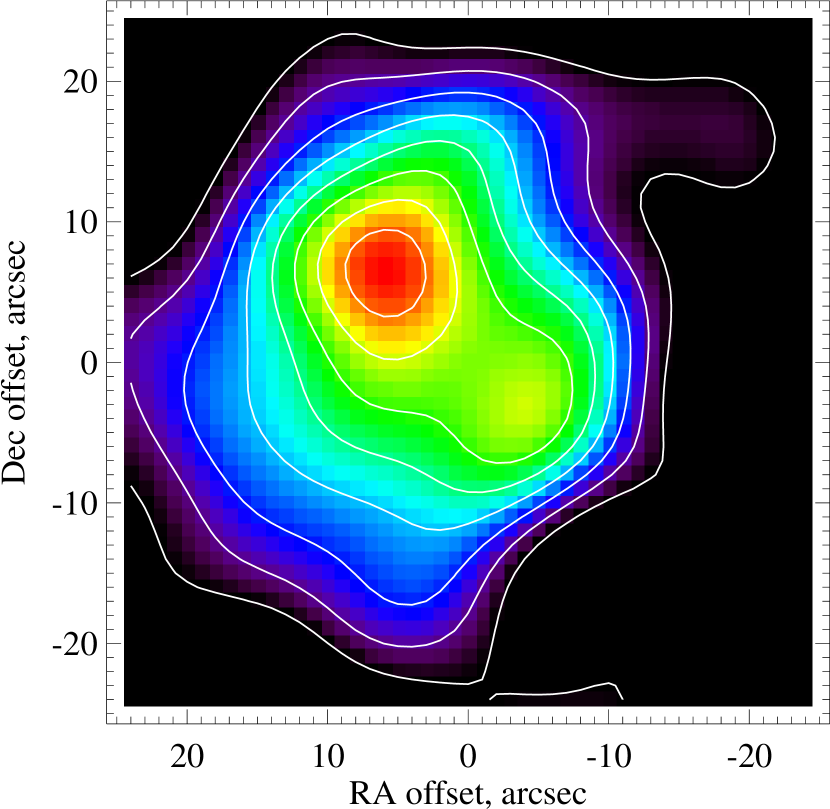
(b)

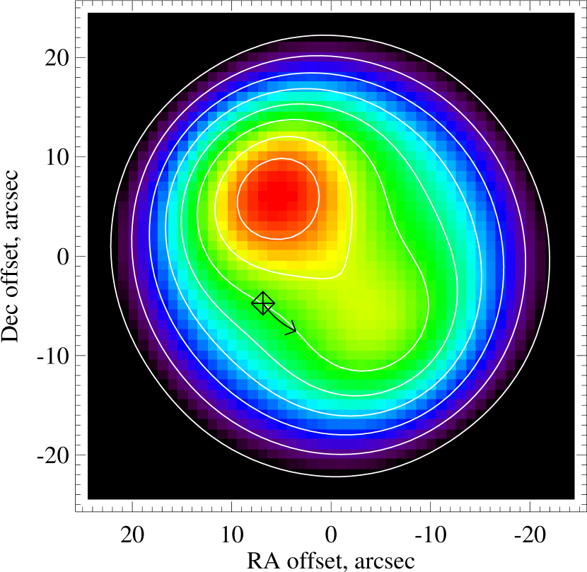
Figure 14: 850 $\mu$m images of Vega. (a) Observation taken using SCUBA at the JCMT (Holland et al. 1998). The contours start at 3.8 mJy beam^-1 and increase at 1.9 mJy beam^-1 intervals. The beam size has a $14\arcsec$ FWHM, and additional gaussian smoothing of $7\arcsec$ FWHM has been applied. Emission from the stellar photosphere of $\sim 5.9$ mJy has not been subtracted from the image. (b) Simulated model image of dust grains created in the destruction of planetesimals shown in Figure 15. The planet is shown at the location of the diamond-plus and its direction of motion is also shown. Appropriate color table, contours, smoothing and stellar photosphere have been included to allow a direct comparison with (a).

Vega is a nearby (7.8 pc) main sequence A0 star ($M_{\star}\approx 2.5M_{\odot}$) with an age of $\sim 350$ Myr (Song et al. 2001). Its emission spectrum exhibits a strong excess above the level of the photosphere at wavelengths longward of 12 $\mu$m (Aumann et al. 1984). This excess originates in dust grains orbiting the star that are continually replenished by the destruction of larger planetesimals in its debris disk. Imaging at submillimeter wavelengths shows the morphology of the excess emission (Holland et al. 1998; see Fig. 14a) down to a resolution of $14\arcsec$ (FWHM): the lowest contours are nearly circularly symmetric extending to $\sim 24\arcsec$, indicating that the disk is being observed pole-on, but the disk’s structure is dominated by an emission peak $\sim 9\arcsec$ to the northeast of the star; the highest contours are also elongated in the southwest direction.

The structure of the disk was recently mapped with even higher spatial resolution ($\sim 3\arcsec$) using millimeter interferometry (Koerner, Sargent & Ostroff 2001; Wilner et al. 2002). While these observations were not sensitive to the larger scale structure, they did show that a significant fraction of the millimeter emission could be resolved into two clumps, one $9.5\arcsec$ northeast of the star, the other $8\arcsec$ southwest of the star, and that the northeast clump is brighter than that southwest. Thus it appears that the submillimeter images are best interpreted as emission from an extended disk which is dominated by two roughly equidistant clumps of unequal brightness on opposite sides of the star.

Based on the discussion of §5.2, the migration zone (Fig. 11) causing this structure can be narrowed down to zone Di: Two clumps of equal brightness could have been explained by planetesimals trapped in the 3:2 resonance (zone C), or in equal numbers into the 2:1(u) and 2:1(l) resonances (zones Dii or Eii), but the asymmetry indicates that one of the clumps is overpopulated, pointing to migration zone Di or Ei. Further constraints are set by the lack of evidence for an additional 3 clump pattern rotated relative to the two clump pattern. While 3 clumps from the 4:3 resonance are inevitable, zone Ei is ruled out as trapping of planetesimals into the 5:3 resonance in this zone means there are less available to be trapped into the 2:1(u) resonance. In theory the outcome of migrations anywhere within zone Di will be similar and are not constrained by this model, however the fuzzy edges of the zones mean that further constraints are possible. Here I set the mass of the planet to be the same as that of Neptune, $M_{pl}=17.2M_{\oplus}$ ($\mu=6.9$), which means that the migration rate must be close to 0.5 AU Myr^-1.

The remaining parameters were then constrained by a best fit to the submillimeter disk image presented in Holland et al. (1998) and reproduced in Figure 14a: the only variables were $a_{max}$, $a_{{pl}_{i}}$, $a_{{pl}_{f}}$, and $\dot{a}_{pl}$, since $\delta$ was fixed at -0.5 and $a_{min}$ was set at $a_{{pl}_{i}}$. The observing geometry was assumed to be face-on and the spatial distribution of planetesimals was converted into an image of the dust emission resulting from the destruction of those planetesimals using the following assumptions: (i) that the spatial distribution of the dust exactly follows the distribution of the parent bodies (i.e., so that the cross-sectional area of emitting dust is proportional to the number of planetesimals); (ii) that the grains’ submillimeter emission is $\propto 1/\sqrt{r}$, which is a good approximation for the large grains which contribute to a disk’s submillimeter emission.

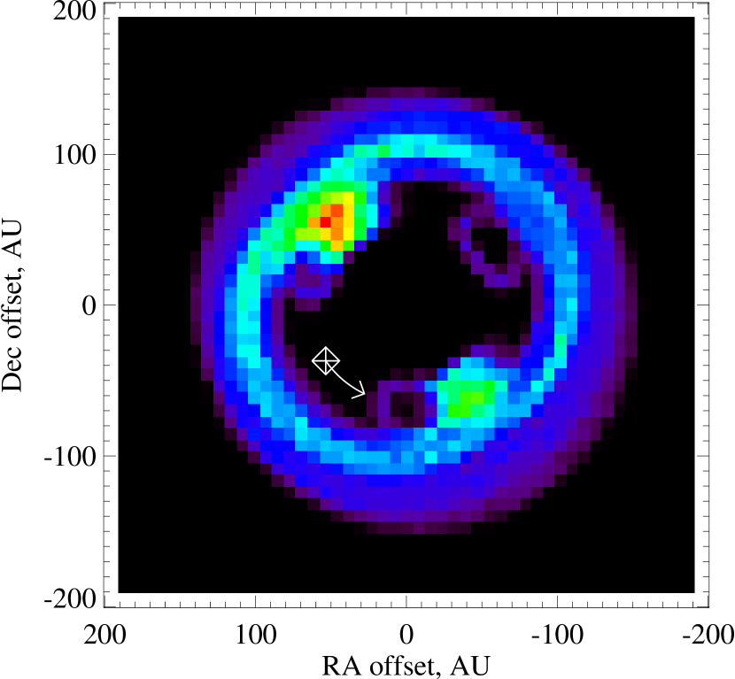
Figure 15: Model of the origin of Vega’s structure as a result of the migration of a Neptune mass planet from 40-65 AU over 56 Myr. (a) The initial and final orbital distribution (eccentricity vs semimajor axis) of planetesimals in the disk. For clarity only the parameters of 200 planetesimals (the asterisks) are shown in this plot. The planet is located at the diamond-plus, the dotted lines indicate the location of the planet’s resonances, and the dashed lines indicate the chaotic resonance overlap region. (b) Image of the number density distribution of planetesimals in the disk at the end of the migration. The planet is located at the diamond-plus.

The resulting best fit is shown in Figure 14b, and was performed by comparison of the contours of the two images; the orbital and spatial distributions of the underlying planetesimal population are shown in Figure 15. The best fit parameters were found to be $a_{max}=140\pm 15$ AU, $a_{{pl}_{i}}=40\pm 10$ AU, $a_{{pl}_{f}}=65\pm 5$ AU, and $\dot{a}_{pl}=0.45\pm 0.1$ AU Myr^-1 (corresponding to $\theta=1.8-3.4$ at 40-140 AU and a total migration time of 56 Myr). In the final distribution 5.1% of the planetesimals are trapped in the 4:3 resonance, 22.5% in the 3:2 resonance, 0.4% in the 5:3 resonance, 18.6% in the 2:1(u) resonance, 0.7% in the 2:1(l) resonance, 41.0% remain in nonresonant orbits, while 11.6% are ejected by resonance overlap. The outer edge of the disk, $a_{max}$, was constrained to within $\sim 15$ AU by a fit to the lowest contours in the images. The final planet location, $a_{{pl}_{f}}$, was constrained to within $\sim 5$ AU by the radial offset of the northeast clump. The contrast of the clumps as well as their morphology were then used to constrain the initial location of the planet, $a_{{pl}_{i}}$, and the migration rate, $\dot{a}_{pl}$. Since the best fit has a migration rate for which trapping into the 2:1 resonance is $<100$%, and into the 5:3 resonance is $>0$%, small changes in $\dot{a}_{pl}$ of the order $\pm 0.02$ AU Myr^-1 resulted in large changes in the model structure. However, $\dot{a}_{pl}$ could not be so well constrained, because the extent of the migration, and so $a_{{pl}_{i}}$, also has a large effect on the model structure, since this determines both the fraction of planetesimals in each resonance as well as their eccentricity distributions. The errors given above are not formal errors, but approximate limits for which acceptable fits are possible to the structure of Figure 14a.

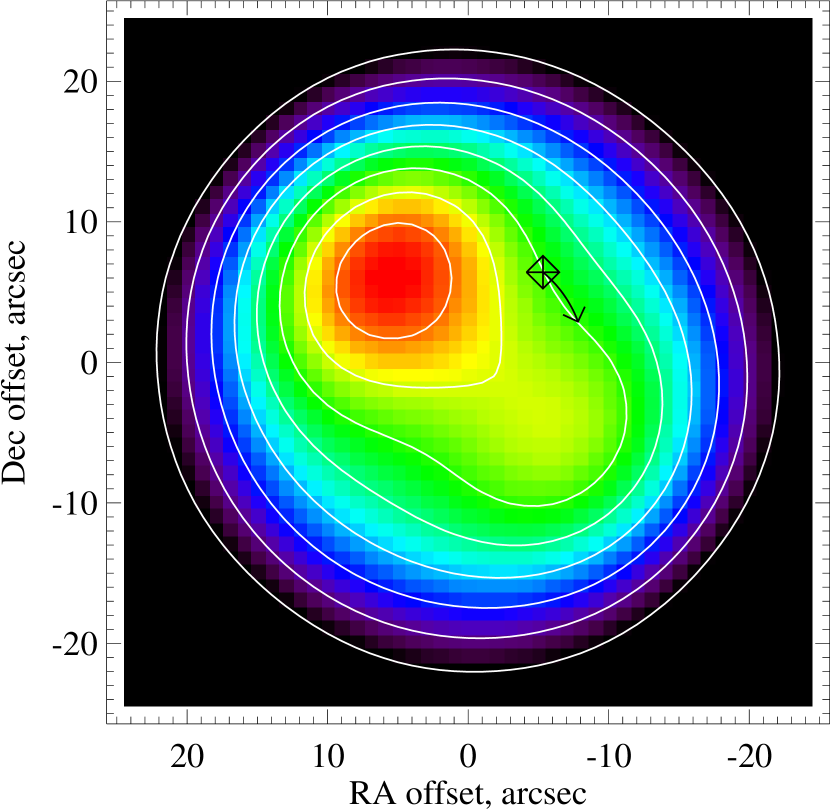
Figure 16: Alternative model explaining the 850 $\mu$m image of Vega’s disk in which the planet causing the structure orbits the star clockwise (see Fig. 14).

This demonstrates that this model can fit the observations very well and in doing so constrains important parameters regarding the evolution of this system. The implications of this model are as follows. First of all the whole pattern is expected to orbit the star with the same period as the planet. As this is predicted to be at 65 AU, the orbital period is 330 yr. Since the clumps are $\sim 9\arcsec$ from the star, their motion would be $0\farcs 17$ yr^-1. With an absolute pointing uncertainty of $\pm 2\arcsec$ from the James Clerk Maxwell Telescope, such absolute motion would not be detectable for several decades in submillimeter images with current technology. However, it would be easier to detect the relative motion of the two clumps, since the position angle of this structure should vary at $1.1^{\circ}$ yr^-1. The direction of the orbital motion presented in Figure 14 is anticlockwise. However this solution is not unique, since the model is nearly symmetrical about the line joining the two clumps, and I could also have modeled the system with clockwise orbital motion, in which case the planet would be currently north of the star. Such a model is shown in Figure 16; there are only slight differences in the disk structure compared with Figure 14b. The important point is that the brighter clump, corresponding to the 2:1(u) resonant planetesimals, trails some $75^{\circ}$ degrees in longitude behind the planet.

Another implication of the model is that the emission distribution is much more intricate than that detectable with a $14\arcsec$ beam. It is therefore interesting that in interferometric images of Vega (Koerner et al. 2001), the northeast clump splits into three, with two lower level clumps straddling a brighter clump; the brighter clump in the model presented in this paper is expected to be extended in longitude (see Figure 15b). This model also makes the prediction that a lower level three clump pattern exists from planetesimals in the 4:3 resonance. While two of the clumps almost blend with the two brighter clumps from the 3:2 and 2:1 planetesimals, a faint clump is expected on the opposite side of the star from the planet. If the presence of such a clump could be inferred from higher resolution and sensitivity observations of this disk, the location of the planet and its direction of motion could be unambiguously determined.

The mass and migration rate of the planet have been constrained to lie at the lower edge of zone Di of Figure 11, although an additional constraint is that the migration rate must be $>0.07$ AU Myr^-1 for the 25 AU migration to have been completed over the age of the system. Thus the planet mass and migration rate I chose is not unique and must be determined by a study of the origin of the migration rate. However, it is noteworthy that in Hahn & Malhotra (1999), Neptune was found to migrate from 23-30 AU over 50 Myr in their model with an initial planetesimal disk mass of $50M_{\oplus}$, a migration rate not too dissimilar to that chosen for this model. In other words, the mass and migration rate of the planet causing the structure of Vega’s disk could be similar to the mass and migration rate of Neptune in our own system. This similarity to the solar system is contrary to previous models for Vega’s disk structure, which was interpreted as dust grains migrating in toward the star due to Poynting-Robertson drag that get trapped into the 2:1 and 3:1 resonances of a 3 Jupiter mass planet on an orbit with an eccentricity of 0.6 (Wilner et al. 2002).

As for the possibility of directly detecting this planet, observational constraints have recently been set on the presence of planets around Vega, with an upper limit of $\sim 3300M_{\oplus}$ at $10\arcsec$ from the star (Metchev, Hillenbrand & White 2003). Given its proximity to the bright star Vega, it would be very difficult to detect this planet with current technology if it is indeed as small as $17M_{\oplus}$. A larger planet, with a necessarily much faster migration rate, may be detectable.

5.4 Caveats

Despite the complexity of the model, it is still just a first step toward a complete explanation of the structures which could be caused in extrasolar systems by planet migration.

For a start, the trapping probabilities were derived for migration through a dynamically cold disk ($e<0.01$). The planetesimals’ eccentricities have a significant influence on trapping probabilities, which decrease as the eccentricities are increased, and also do not reach a maximum at 100% trapping probability for low migration rates if the eccentricity is above a certain threshold (Borderies & Goldreich 1984; Melita & Brunini 2000). Most importantly, the trapping probabilities of different resonances are affected in different ways, with higher order ($q>1$) resonances becoming more populated relative to lower order resonances for higher eccentricities. Indeed Chiang et al. (2003) propose that the Kuiper belt must have been dynamically hot ($e\approx 0.2$) when the migration of Neptune occurred to explain the presence of three KBOs in the 5:2 resonance given that only seven objects have been discovered in Neptune’s 2:1 resonance. It is difficult to predict an appropriate eccentricity distribution for the residual planetesimal disk. While planetesimals are thought to form in a dynamically cold disk, the sweeping of a planet’s resonances and its secular perturbations, as well as scattering of planetesimals from closer to the star, can all contribute to increasing the average eccentricity of the planetesimal disk. Certainly future models will have to consider the possibility of high eccentricities, but in doing so will become more complicated, since trapping into higher order resonances will also have to be considered.

Another omission of the model is stochastic effects. Migration in the models of Hahn & Malhotra (1999) is not smooth, but shows large jumps. This is because the residual planetesimals used in their simulation had to be large to give reasonable integration times. If the most massive residual planetesimals causing migration are smaller than a certain limit, then stochastic effects can be ignored (Chiang et al. 2003), otherwise they must be characterized (Zhou et al. 2002). One reason for anticipating that the residual planetesimals causing the migration are much smaller than the planet would be if the planet formed much closer to the star than the planetesimals. This could be the case if the planet was flung out in a gravitational interaction with other giant planets (Thommes et al. 2002) or migrated out to a more distant location.

Possibly the most worrying aspect of the model is the translation of the distribution of planetesimals to the distribution of dust. These were assumed to be identical, but this may not be exactly true. For a start the radial location of the resonances are different for small dust, since they orbit the star slower than larger grains due to radiation pressure (Wyatt et al. 1999). Also, these particles have different orbits from their parents, not only because of radiation pressure, but also due to the velocity given to them during the collision. The effect of P-R drag and subsequent collisions should also be taken into account. These are important issues, but ones which merit a paper in themselves. However, in defense of this assumption I will point out two things. First, the dust which contributes to the submillimeter images is expected to be large, since small grains emit very inefficiently at such long wavelengths (Wyatt & Dent 2002). Second, most resonant planetesimals are on planet-crossing orbits (i.e., $a_{res}(1-e_{res})<a_{pl}$), and the only reason such orbits are stable is because resonant forces prevent a close approach (§4). Small dust originating from such planetesimals, but which is no longer in resonance, would therefore be expected to be short-lived, since without the protection of the resonance a close approach to the planet is possible resulting in scattering out of the system. Such scattering is confirmed in more recent runs following the evolution of the dust particles’ orbits (Wyatt, in prep.).

Another concern is that the dust distribution may be affected by random events in which single massive planetesimals are disrupted. Such events may have been witnessed in the structure of the zodiacal cloud (Dermott et al. 2002; Nesvorný et al. 2003). However, Wyatt & Dent (2002) concluded that inidividual collisions are unlikely to be a significant source of structure in the Fomalhaut disk (which also contains a clump, Holland et al. 2003), since this disk is so massive that only a collision between two planetesimals at least 1400 km in diameter could affect its structure at the level observed, and too few such planetesimals can coexist in the disk. Since Vega’s disk, and its clumps, have a similar mass to those of Fomalhaut (Holland et al. 1998), I conclude that random collisions are also unlikely to be the cause of Vega’s clumpy disk structure.

While I prefer to leave the discussion of the origin of the planet’s migration to a later paper, it is worth pointing out that only certain values of $\theta$ will be possible for a given planet mass $\mu$ and initial planetesimal disk mass (Hahn & Malhotra 1999). In other words, the planet’s mass and migration rate, as well as the initial mass of Vega’s planetesimal disk, could be much better constrained with a model incorporating both migration and resonant trapping. Also, in the models of the migration of the solar system’s planets, Neptune’s migration is outward only because of the existence of the massive planets interior to its orbit. This is because the planetesimals scattered inwards by Neptune (causing its outward migration) may not return for a subsequent scattering event (causing inward motion) due to their interaction with the closer in planets, whereas the converse is not true. Thus an outward migration may be said to be indicative of at least two planets. However, Ida et al. (2000) presented an analytical model for planet migration claiming that once outward migration has started, it is self-sustaining, since there are automatically less planetesimals interior to the planet’s orbit.

6 Conclusion

I have presented a model describing the consequence of the outward migration of a planet on the dynamical and spatial structure of a planetesimal disk residing outside the planet’s orbit. In §3 numerical simulations were used to show how trapping probabilities into the 4:3, 3:2, 5:3, and 2:1 resonances can be estimated to within 5% given just two parameters $\mu=M_{pl}/M_{\star}$ and $\theta=\dot{a}_{pl}\sqrt{a/M_{\star}}$. Resonant forces cause a planetesimal’s resonant argument, $\phi$, to librate and in §4 physical arguments were used to explain what azimuthal structure is expected in the distribution of planetesimals as a result of this libration: planetesimals trapped in the 4:3 and 5:3 resonances are concentrated at 60, 180, and 300^∘ longitude relative to the planet, those in the 3:2 resonance are concentrated at $\pm 90^{\circ}$ longitude, and those in the 2:1 resonance are concentrated in two clumps associated with the 2:1(u) resonance with a concentration at relative longitude of $\sim 285^{\circ}$, and the 2:1(l) resonance with a concentration at $\sim 75^{\circ}$. Also in §4, numerical simulations were used to show how the angle about which $\phi$ librates, as well as the amplitude of that libration, are affected by the migration parameters. These simulations also characterized the overpopulation of the 2:1(u) resonance relative to the 2:1(l) for different migrations. In §5 the numerical results were used to derive a numerical scheme to predict the spatial distribution of planetesimals resulting from a migration defined by $\mu$ and $\theta$. It was shown that the dynamical structure of a post-migration disk can have one of seven states depending on the $\mu$ and $\theta$ of the migration.

Application of the model to the structure of Vega’s debris disk presented in Holland et al. (1998) shows that its two clumps of unequal brightness can be explained by the migration of a Neptune mass planet from 40-65 AU over $\sim 56$ Myr through a planetesimal disk initially extending from 40-140 AU. The two clumps are caused by planetesimals trapped in the 3:2 and 2:1 resonances, and the brightness asymmetry is caused by an overabundance of planetesimals in the 2:1(u) resonance relative to the 2:1(l) resonance. While the extent of the planet’s migration is well constrained by the brightness of the clumps, its mass and migration rate are not unique, although they are constrained to lie within certain ranges defined by zone Di in Figure 11. Further constraints on the planet’s mass and migration rate, as well as on the mass of the planetesimal disk, would be possible by modeling the origin of the planet’s migration in angular momentum exchange with the planetesimal disk. Predictions of the model which may prove its validity are the orbital motion of Vega’s clumpy pattern ($1.1^{\circ}$ yr^-1), the location of the planet ($8\farcs 3$ from the star, $75^{\circ}$ in longitude in front of the orbital motion of the NE clump), and the high resolution structure of the clumps including the presence of a fainter third clump on the opposite side of the star from the planet from planetesimals in the 4:3 and 5:3 resonances.

While the mass and migration rate of Vega’s perturbing planet are not yet fully constrained, the migration parameters derived for Neptune in the solar system (Hahn & Malhotra 1999) are close to the small region of parameter space which could have caused Vega’s structure. There is also an intriguing suggestion that a planet’s outward migration requires the presence of massive planets interior to its orbit. Thus it seems possible that Vega’s planetary system is very similar to our own, not only in the presence and mass of the planets in its system, but in that system’s early evolution. It is also possible that application of this model to the other clumpy debris disks may show these to harbor solar-like planetary systems. The weight of such conclusions is damped only by the limitations of the model. These will be addressed in future studies, and include questions about the extent the dust distribution follows that of the parent planetesimals, and how the conclusions are affected if the planetesimal disk is initially dynamically hot ($e>0.01$).

Appendix A Adiabaticity

As a result of the fit to the libration of $\phi$ performed in §4.3, the libration period for each planetesimal, $t_{\phi}$ was also determined for all resonant planetesimals in each run, as was the mean libration period of the ensemble, $\langle t_{\phi}\rangle$. The results are plotted in Figure 17. Fits to these were performed of the form $(\langle t_{\phi}\rangle/t_{per})\sqrt{\mu}=A/e^{B}+C\theta/\mu$, where $t_{per}$ is the orbital period of the planetesimal and $B=0$ except for the 2:1 resonance. These showed that

$$\langle t_{{\phi}_{2:1}}\rangle/t_{per} = 78.9\mu^{-0.5}e^{-0.9},$$ (A1)

$$\langle t_{{\phi}_{5:3}}\rangle/t_{per} = 317\mu^{-0.5}-86.4\theta\mu^{-1.5},$$ (A2)

$$\langle t_{{\phi}_{3:2}}\rangle/t_{per} = 412\mu^{-0.5}-7.7\theta\mu^{-1.5},$$ (A3)

$$\langle t_{{\phi}_{4:3}}\rangle/t_{per} = 307\mu^{-0.5}-5.2\theta\mu^{-1.5},$$ (A4)

and these fits are also shown on Figure 17. So, the libration period for the 2:1 resonance is not affected by the planet’s migration rate, but it does decrease during the migration as the planetesimal’s eccentricity increases. However, for the 5:3, 3:2, and 4:3 resonances, the libration period is constant throughout the migration, but does depend on the $\mu$ and $\theta$ of the migration in that faster migrations (and larger planet masses) result in smaller libration periods.

The libration width for each planetesimal, $\Delta a=a_{max}-a_{min}$, was also measured, as was the mean libration width $\langle\Delta a\rangle$. Since the runs for the 3:2 resonance showed that $\Delta a$ is not just dependent on $\mu$ and $\theta$, but also on $M_{\star}$ which was not varied for the other resonances, I only attempted to characterize the libration width for the 3:2 resonance (see also Figure 18):

$$\langle\Delta a_{3:2}\rangle/a=0.0023\theta\mu^{-0.44}M_{\star}^{-0.9}.$$ (A5)

The mean libration widths for all resonances were used, however, to question the adiabaticity of this libration. Adiabaticity is defined as when the libration period, $t_{\phi}$, is much shorter than the time it takes for the resonance to cross the libration width, i.e., $t_{\phi}\ll\Delta a/\dot{a}_{pl}$. I found that in the runs shown here, $N_{lib}=(\Delta a/\dot{a}_{pl})/t_{\phi}$ was in the ranges: $1.5-15$ for the 3:2 resonance; $2.5-3.9$ for the 4:3 resonance; $10-400$ for the 5:3 resonance; and $3.6-25$ for the 2:1 resonance. In other words, all the migrations considered in this paper satisfy adiabatic invariance (Henrard 1982), though many are close to this limit.

(a)
(b)
(c)

Figure 1: Capture probabilities for the 3:2 resonance for planetesimals initially orbiting at 60 AU from a $2.5M_{\odot}$ star plotted for different mass planets that are migrating at different rates (a) (see §3.1.1). The solid lines show fits to these probabilities using the function given in equation (3). Parameters derived from these fits are shown in (b) and (c). (b) shows the migration rate required for a planet to capture a given fraction of the planetesimals in its 3:2 resonance, while $\gamma$ in (c) defines how fast the capture probability drops with migration rate for a given planet mass.

(a)
(b)
(c)

Figure 2: Capture probabilities for the 3:2 resonance of a $10M_{\oplus}$ planet for planetesimals initially orbiting at different distances from a $2.5M_{\odot}$ star (a) (see §3.1.2). The solid lines show fits to these probabilities using the function given in equation (3). Parameters derived from these fits are shown in (b) and (c).

(a)
(b)
(c)

Figure 3: Capture probabilities for the 3:2 resonance of a $10M_{\oplus}$ planet for planetesimals initially orbiting at 60 AU from stars of different mass (a) (see §3.1.3). The solid lines show fits to these probabilities using the function given in equation (3). Parameters derived from these fits are shown in (b) and (c).

(a)
(b)
(c)

Figure 4: Capture probabilities for planetesimals initially 30 AU from a $2.5M_{\odot}$ star for trapping into the (a) 2:1, (b) 4:3, and (c) 5:3 resonances. The solid lines show fits to these probabilities for each planet mass using equation (3). The dotted lines show the fit to the capture probabilities using equation (8).

Figure 5: Summary of capture probabilities for the 4:3, 3:2, 2:1, and 5:3 resonances for migrations defined by the parameters $\mu$ and $\theta$ (eqs. [6]-[8] with parameters from Table 1). The dotted, solid, and dashed lines indicate migrations for which trapping probabilities are 10, 50, and 90% respectively. The dash-triple dot line indicates migrations for which the 2:1(u) resonance has twice as many members as the 2:1(l) resonance (see §4.3.4).

	$e=0.1$	$e=0.2$	$e=0.3$
2:1
5:3
3:2
4:3

Figure 6: Paths of resonant orbits in the frame co-rotating with the mean motion of the planet. The planet is marked by a cross in these figures and it is stationary in this reference frame, since its orbit is circular. Crosses show the location of a planetesimal in the different resonances (2:1, 5:3, 3:2, and 4:3) at intervals of 1/24th of the planet’s orbital period (i.e., when the planet has moved by $15^{\circ}$ in the inertial frame). The planet moves anticlockwise in the inertial frame, and the planetesimals move anticlockwise in this reference frame. Sufficient crosses are marked to show how this pattern repeats itself, which is every $p+q$ orbits of the planet. The three plots for each resonance show the paths for planetesimal eccentricities of 0.1, 0.2, and 0.3. Naturally, these plots show just one value of the planetesimal’s pericenter, which always occurs at the same location in inertial space, but occurs $p$ times in the rotating frame plots (at the innermost point of the loops). Resonant orbits with different pericenters, which can be specified by the resonant angle $\phi$ (eq. [11]), would show the same pattern, but rotated on this figure by an angle $\phi/p$. The three plots for the 2:1 resonance have $\phi=257$, 275, and $281^{\circ}$ (for increasing eccentricity), while the remainder have $\phi=180^{\circ}$ (see §4.3.3).

(a)
(b)
(c)

Figure 7: Offset of the mean libration centers, $\langle\phi_{m}\rangle$, from $180^{\circ}$ for planetesimals trapped in the (a) 5:3, (b) 3:2, and (c) 4:3 resonances as a result of planet migration defined by the parameters $\mu$ and $\theta$ (eqs. [6] and [7]). The solid lines show the fits to these offsets for each resonance given in equations (23)-(25).

Figure 8: Variation of the mean libration center, $\langle\phi_{m}\rangle$, as a result of planet migration for planetesimals trapped in the 2:1(u) and 2:1(l) resonances. The solid line shows the fit to this variation given in equation (26). The analytical solution given in equation (19) is shown with the dotted line.

Figure 9: Capture probabilities for the 2:1(l) resonance, $P_{2:1(l)}$, for planetesimals initially 30 AU from a $2.5M_{\odot}$ star. The parameterised fits to these probabilities given in equations (27) and (28) for the four planet masses shown in this plot (i.e., $\mu=4$, 12, 40, and 120) are shown with dashed lines.

(a)
(b)
(c)
(d)

Figure 10: Mean libration amplitudes, $\langle\Delta\phi\rangle$, of planetesimals captured in the (a) 2:1, (b) 5:3, (c) 3:2, and (d) 4:3 resonances for migrations defined by the parameters $\mu$ and $\theta$ (eqs. [6] and [7]). The solid lines show the fits to these libration amplitudes given in equations (33)-(36).

Figure 11: Definition of the migration zones A-Eii discussed in the text and Table 2. The lines are the same as those in plotted in Figure 5.

Figure 12: Rotation (clockwise) of the resonant pattern shown in Figure 6 due to the migration of the planet characterized in Figure 7. This is shown for migrations resulting in trapping probabilities of 10, 50, and 90%.

(a)
(b)

Figure 13: Libration amplitudes for migrations resulting in trapping probabilities of 10, 50, and 90% for: (a) the 5:3, 3:2, and 4:3 resonances; (b) the 2:1 resonance when $e=0.03$ and 0.3.

(a)
(b)

(a)
(b)
(c)
(d)

Figure 17: Mean libration periods, $\langle t_{\phi}\rangle/t_{per}$, of planetesimals captured in the (a) 2:1, (b) 5:3, (c) 3:2, and (d) 4:3 resonances for migrations defined by the parameters $\mu$ and $\theta$ (eqs. [6] and [7]). The solid lines show the fits to these libration periods given in equations (A1)-(A4).

Figure 18: Mean libration width, $\langle\Delta a\rangle/a$, of planetesimals captured in the 3:2 resonance for migrations defined by the parameters $\mu$ and $\theta$ (eqs. [6] and [7]) for stellar masses $M_{\star}$. The solid line shows the fit to these libration widths given in equation (A5).

Table 1: Coefficients that determine capture probabilities from equation (8) for different resonances (§3). Also given are the semimajor axes of the resonances, $a_{r}$, with respect to that of the perturbing planet, $a_{pl}$, and the average errors in the capture probabilities using these models, $P_{err}$.

Resonance	$a_{r}/a_{pl}$	$X$	$Y$	$u$	$v$	$P_{err}$
4:3	1.21	$0.23\pm 0.02$	$5.6\pm 2.0$	$1.42\pm 0.01$	$0.29\pm 0.1$	0.05
3:2	1.31	$0.37\pm 0.02$	$5.4\pm 2.0$	$1.37\pm 0.01$	$0.38\pm 0.1$	0.04
5:3	1.41	$210\pm 20$	$1.0\pm 0.2$	$1.84\pm 0.02$	$0.20\pm 0.08$	0.04
2:1	1.59	$5.8\pm 0.2$	$4.3\pm 2.0$	$1.40\pm 0.02$	$0.27\pm 0.2$	0.025

Table 2: Which resonances planetesimals initially at semimajor axes of $a_{i}$ end up in given the initial semimajor axis of the planet $a_{{pl}_{i}}$ for the different migration scenarios A-Eii shown in Figure 11. Also given are the longitudes of the concentrations of planetesimals in the different resonances relative to the planet, $\lambda-\lambda_{pl}$.

Resonance	2:1(u)	2:1(l)	5:3	3:2	4:3
$\lambda-\lambda_{pl}$	$-(107-79^{\circ})$	$(107-79^{\circ})$	$\pm 60^{\circ},180^{\circ}$	$\pm 90^{\circ}$	$\pm 60^{\circ},180^{\circ}$
A	-	-	-	-	-
B	-	-	-	-	$a_{i}>1.21a_{{pl}_{i}}$
C	-	-	-	$a_{i}>1.31a_{{pl}_{i}}$	$a_{i}=(1.21-1.31)a_{{pl}_{i}}$
Di	$a_{i}>1.59a_{{pl}_{i}}$	-	-	$a_{i}=(1.31-1.59)a_{{pl}_{i}}$	$a_{i}=(1.21-1.31)a_{{pl}_{i}}$
Dii	50% of $a_{i}>1.59a_{{pl}_{i}}$	50% of $a_{i}>1.59a_{{pl}_{i}}$	-	$a_{i}=(1.31-1.59)a_{{pl}_{i}}$	$a_{i}=(1.21-1.31)a_{{pl}_{i}}$
Ei	$a_{i}>1.59a_{{pl}_{i}}$	-	$a_{i}=(1.41-1.59)a_{{pl}_{i}}$	$a_{i}=(1.31-1.41)a_{{pl}_{i}}$	$a_{i}=(1.21-1.31)a_{{pl}_{i}}$
Eii	50% of $a_{i}>1.59a_{{pl}_{i}}$	50% of $a_{i}>1.59a_{{pl}_{i}}$	$a_{i}=(1.41-1.59)a_{{pl}_{i}}$	$a_{i}=(1.31-1.41)a_{{pl}_{i}}$	$a_{i}=(1.21-1.31)a_{{pl}_{i}}$

References

- Augereau et al. (2001) Augereau, J. C., Nelson, R. P., Lagrange, A. M., Papaloizou, J. C. B., & Mouillet, D. 2001, A&A, 370, 447
- Aumann et al. (1984) Aumann, H. H., et al. 1984, ApJ, 278, L23
- Backman & Paresce (1993) Backman, D. E., & Paresce, F. 1993, in Protostars and Planets III, ed. E. H. Levy & J. I. Lunine (Tucson: Univ. Arizona Press), 1253
- Beaugé (1994) Beaugé, C. 1994, CeMDA, 60, 225
- Borderies & Goldreich (1984) Borderies, N., Goldreich, P. 1984, CeMDA, 32, 127
- Burns et al. (1979) Burns, J. A., Lamy, P. L., & Soter, S. 1979, Icarus, 40, 1
- Chiang & Jordan (2002) Chiang, E. I., & Jordan, A. B. 2002, AJ, 124, 3430
- Chiang et al. (2003) Chiang, E. I., et al. 2003, AJ, in press
- Dermott et al. (1994) Dermott, S. F., Jayaraman, S., Xu, Y. L., Gustafson, B. A. S., & Liou, J. C. 1994, Nature, 369, 719
- Dermott et al. (2002) Dermott, S. F., Kehoe, T. J. J., Durda, D. D., Grogan, K., Nesvorný, D. 2002, in Proceedings of Asteroids, Comets, Meteors (ACM 2002), ed. B. Warmbein (Noordwijk: ESA Publications Division), 319
- Everhart (1985) Everhart, E. 1985, in Dynamics of Comets, ed. A. Carusi & G. B. Valsecchi (Dordrecht: Reidel), 185
- Fernández & Ip (1984) Fernández, J. A., & Ip, W.-H. 1984, Icarus, 58, 109
- Friedland (2001) Friedland, L. 2001, ApJ, 547, L75
- Gomes (2003) Gomes, R. S. 2003, Icarus, 161, 404
- Greaves et al. (1998) Greaves, J. S., et al. 1998, ApJ, 506, L133
- Hahn & Malhotra (1999) Hahn, J. M., & Malhotra, R. 1999, AJ, 117, 3041
- Heap et al. (2000) Heap, S. R., Lindler, D. J., Lanz, T. M., Cornett, R. H., Hubeny, I., Maran, S. P., & Woodgate, B. 2000, ApJ, 539, 435
- Henrard (1982) Henrard, J. 1982, CeMDA, 27, 3
- Henrard & Lemaitre (1983) Henrard, J., & Lemaitre, A. 1983, CeMDA, 30, 197
- Holland et al. (1998) Holland, W. S., et al. 1998, Nature, 392, 788
- Holland et al. (2003) Holland, W. S., et al. 2003, ApJ, 582, 1141
- Ida et al. (2000) Ida, S., Bryden, G., Lin, D. N. C., & Tanaka, H. 2000, ApJ, 534, 428
- Jewitt (1999) Jewitt, D. 1999, Ann. Rev. Earth Planet. Sci., 27, 287
- Kenyon & Bromley (2002) Kenyon, S. J., & Bromley, B. C. 2002, ApJ, 577, L35
- Koerner, Sargent & Ostroff (2001) Koerner, D. W., Sargent, A. I., & Ostroff, N. A. 2001, ApJ, 560, L181
- Kuchner & Holman (2003) Kuchner, M. J., & Holman, M. J. 2003, ApJ, 588, 1110
- Laureijs et al. (2002) Laureijs, R. J., Jourdain de Muizon, M., Leech, K., Siebenmorgen, R., Dominik, C., Habing, H. J., Trams, N., & Kessler, M. F. 2002, å, 387, 285
- Malhotra (1995) Malhotra, R. 1995, AJ, 110, 420
- Malhotra (1996) Malhotra, R. 1996, AJ, 111, 504
- Melita & Brunini (2000) Melita, M. D., & Brunini, A. 2000, Icarus, 147, 205
- Metchev, Hillenbrand & White (2003) Metchev, S. A., Hillenbrand, L. A., White, R. J. 2003, ApJ, 582, 1102
- Moro-Martín & Malhotra (2002) Moro-Martín, A., & Malhotra, R. 2002, AJ, 124, 2305
- Murray & Dermott (1999) Murray, C. D., & Dermott, S. F. 1999, Solar System Dynamics (Cambridge: Cambridge University Press)
- Nesvorný et al. (2003) Nesvorný, D., Bottke, W. F., Levison, H. F., Dones, L. 2003, ApJ, 591, 486
- Ozernoy et al. (2000) Ozernoy, L. M., Gorkavyi, N. N., Mather, J. C., & Taidakova, T. A. 2000, ApJ, 537, L147
- Peale (1976) Peale, S. J. 1976, ARA&A, 14, 215
- Quillen & Thorndike (2002) Quillen, A. C., & Thorndike, S. 2002, ApJ, 578, L149
- Song et al. (2001) Song, I., Caillault, J.-P., Barrado y Navascués, D., Stauffer, J. R. 2001, ApJ, 546, 352
- Telesco et al. (2000) Telesco, C. M., et al. 2000, ApJ, 530, 329
- Thommes et al. (2002) Thommes, E. W., Duncan, M. J., & Levison, H. F. 2002, AJ, 123, 2862
- Wilner et al. (2002) Wilner, D. J., Holman, M. J., Kuchner, M. J., & Ho, P. T. P. 2002, ApJ, 569, L115
- Wisdom (1980) Wisdom, J. 1980, AJ, 85, 1122
- Wyatt & Dent (2002) Wyatt, M. C., & Dent, W. R. F. 2002, MNRAS, 334, 589
- Wyatt et al. (1999) Wyatt, M. C., Dermott, S. F., Telesco, C. M., Fisher, R. S., Grogan, K., Holmes, E. K., & Piña, R. K. 1999, ApJ, 527, 918
- Wyatt et al. (2003) Wyatt, M. C., Holland, W. S., Greaves, J. S., Dent, W. R. F. 2003, Earth Moon Planets, in press
- Zhou et al. (2002) Zhou, L.-Y., Sun, Y.-S., Zhou, J.-L., Zheng, J.-Q., & Valtonen, M. 2002, MNRAS, 336, 520