Towards a complete theory of Gamma Ray Bursts

Abstract

Gamma Ray Bursts (GRBs) are notorious for their diversity. Yet, they have a series of common features. The typical energy of their $\gamma$ rays is a fraction of an MeV. The energy distributions are well described by a “Band spectrum”, with “peak energies” spanning a surprisingly narrow range. The time structure of a GRB consists of pulses, superimposed or not, rising and decreasing fast. The number of photons in a pulse, the pulses’ widths and their total energy vary within broad but specific ranges. Within a pulse, the energy spectrum softens with increasing time. The duration of a pulse decreases at higher energies and its peak intensity shifts to earlier time. Many other correlations between pairs of GRB observables have been identified. Last (and based on one measured event!) the $\gamma$-ray polarization is very large. A satisfactory theory of GRBs should naturally and very simply explain, among others, all these facts. We show that the “cannonball” (CB) model does it. In the CB model the process leading to the ejection of highly relativistic jetted CBs in core-collapse supernova (SN) explosions is akin to the one observed in quasars and microquasars. The prompt $\gamma$-ray emission —the GRB— is explained extremely well by inverse Compton scattering of light in the near environment of the SN by the electrons in the CBs’ plasma. We have previously shown that the CB-model’s description of GRB afterglows as synchrotron radiation from ambient electrons —swept in and accelerated within the CBs— is also simple, universal and very successful. The only obstacle still separating the CB model from a complete theory of GRBs is the theoretical understanding of the CBs’ ejection mechanism in SN explosions.

1 Introduction

Once upon a time there were —literally— some five score and seven theories of gamma-ray bursts (GRBs, see e.g. Nemiroff 1994). In this Dark Era, the observations were scarce, and they were the exclusive realm of a few satellites (VELA, GRANAT, SMM, GINGA). During a good fraction of the last decade of the past century, the BATSE Era, a single detector —the Burst And Transient Satellite Experiment aboard the Compton Gamma Ray Observatory (CGRO) satellite— dominated the data-taking effort (see e.g. Fishman & Meegan 1995). The BATSE team determined that the distribution of GRB arrival directions was extremely isotropic in the sky, a very strong hint that their sources were “cosmological” (Meegan et al. 1992). This reduced the number of tenable GRB theories by a very large factor.

In parallel, or subsequently to the very successful CGRO mission, various $\gamma$- and X-ray satellites —BeppoSAX, Rossi, HETE II, Integral and the Inter-Planetary Network of spacecrafts (Wind, PVO, Ulysses, Mars Odyssey and RHESSI)— were operational and capable of performing faster and more precise directional localizations of GRBs. Following the consequent discovery that the sources of GRBs continue to shine after their transient high-energy pulses (Costa et al. 1997), a quantum leap of information took place. Indeed, a GRB “event” does not end as the $\gamma$-ray flux becomes undetectably small, for there is an “afterglow” (AG): the source continues to emit light at all smaller observable frequencies, ranging from X-rays to radio waves, and to be observable for months, or even years (van Paradijs et al. 1997; Frail et al. 1997). In the Afterglow Era (see e.g. Proc. GRBs in the Afterglow Era, 1999, A&AS, Vol. 138), the fact that these remaining emissions can be very well localized in the sky led to the discovery of the GRBs’ host galaxies (Sahu et al. 1997); to the measurement of their redshifts (Metzger et al. 1997) that verified their cosmological origin; to the identification of their birthplaces —mainly star formation regions in normal galaxies (Holland & Hjorth 1999)— and to the first evidence for a possible physical association between GRBs and supernova explosions: that of GRB 980425 and SN1998bw (Galama et al. 1998).

The possibility to observe the relatively intense early optical AGs, even with rather small telescopes, has had the beneficial effect of enlarging the “GRB community” well beyond its previous bounds. A recent, serendipitous and most-welcome newcomer to the GRB observational community was the satellite RHESSI (Reuven Ramaty High Energy Solar Spectroscopic Imager satellite). Looking with this instrument close to the Sun’s direction, Coburn and Boggs (2003) discovered GRB 021206, and measured a very large linear polarization of its prompt $\gamma$-rays: $\Pi=(80\pm 20)\,\%$. This polarization is much higher than the few per cent values observed in the optical AG of GRBs (GRB 990123: Hjorth et al. 1999; GRB 990510: Wijers et al. 1999; Covino et al. 1999; GRB 990712: Rol et al. 2000; GRB 010222: Bjornsson et al. 2002; GRB 011211: Covino et al. 2002; GRB 020405: Bersier et al. 2003a; Masetti et al. 2003; Covino et al. 2003a; GRB 020813: Covino et al. 2003b; GRB 021004: Rol et al. 2003; Wang et al. 2003; GRB 030329: Efimov et al. 2003; Magalhaes et al. 2003; Covino et al. 2003c).

The influence of the discovery of AGs on the theory of GRBs has been enormous, and not only because we now know that their sources are cosmological, and must —somehow— be related to stars. It is very very difficult to imagine a GRB theory in which there is no sequel to a GRB. In the fireball model (the FB model, in its many variants: Paczynski 1986; Goodman 1986; Shemi & Piran 1990; Narayan, Paczynski & Piran 1992; Rees & Mészáros 1992, 1994; Katz 1994a,b; Mészáros & Rees 1997; Waxman 1997a,b; Dermer & Mitman 1999; for reviews see, e.g. Piran 1999, 2000; Mészáros 2002; Hurley, Sari & Djorgovski 2002; Waxman 2003a), long a leading contender for consideration as the theory of GRBs, the existence of AGs declining in intensity as an inverse power of time had been anticipated (Katz 1994b; Mészáros & Rees 1997; Mészáros, Rees 1997 & Wijers 1998). In the AG era, the FB model rose in consideration to become generally accepted as the standard model of GRBs. Radically different models, such as our “cannonball” (CB) model (Dar & De Rújula 2000a,b; Dado, Dar & De Rújula 2002a, 2003a), were received with considerable skepticism (De Rújula 2003). Even small deviations from the prevailing credo (Dermer & Mitman 1999) met a similar fate (Dermer 2002).

In the FB models, both the prompt $\gamma$-rays and the AG are due to synchrotron radiation from shock-accelerated electrons moving in a chaotic magnetic field. Thus, their very different polarizations were not expected (see, e.g. Gruzinov 1999; Gruzinov & Waxman 1999). A large polarization requires at first sight an ad-hoc magnetic and/or jet structure (Lyutikov, Pariev & Blandford 2003; Waxman 2003b; Eichler & Levinson 2003; Nakar, Piran & Waxman 2003) and is —to say the least— quite a surprise.

The $\gamma$-rays of a GRB may not be produced by synchrotron radiation and their polarization may not necessarily imply a strong, large-scale, ordered magnetic field in their source. In fact, Shaviv and Dar (1995) suggested that highly relativistic, narrowly collimated jets ejected near the line of sight in accretion-induced collapse of stars in distant galaxies may produce cosmological GRBs by inverse Compton scattering (ICS) of stellar light. If the Lorentz factor of the jet is $\gamma\sim 10^{3}$, ICS of isotropic unpolarized stellar light by the electrons in the jet boosts the photons to $\gamma$-ray energies, beams them along the direction of motion of the jet, and results in a large polarization ($\Pi\approx 100\%$ when the jet is viewed close to the most probable viewing angle, $\theta\sim 1/\gamma$). But the density of the radiation field, even in the most dense star-burst regions, was found to be insufficient to explain the $\gamma$-ray fluence of the most powerful GRBs, such as GRB 990213. We shall see that, in the CB model, this problem —the dearth of “target” light— does not arise.

In the CB model, long-duration GRBs are made by core-collapse supernovae (SNe). As we asserted in Dar & De Rújula (2000a) “the light from the SN shell is Compton up-scattered to MeV energies, but its contribution to a GRB is sub-dominant”. That assertion is correct: the light from the SN shell is too underluminous and too radially directed to generate GRBs of the observed fluence and individual-photon energy. With our collaborator Shlomo Dado, we have developed a very complete, simple and —we contend— extremely successful analysis of GRB AGs (Dado, Dar & De Rújula 2002a,b,c, 2003a,b,c,d,e,f). This thorough analysis has taught us that there should be another, much more intense and more isotropic, source of scattered light: the SN’s “glory”. The glory is the “echo” (or ambient) light from the SN, permeating the “wind-fed” circumburst density profile, previously ionized by the early extreme UV flash accompanying a SN explosion, or by the enhanced UV emission that precedes it. In Sections 2 and 3 we summarize the observations of pre-SN winds, early SN luminosities, and the UV flashes of SNe, to obtain the reference values of the very early quantities of interest: the wind’s density $\rho(r)$, and density profile (roughly $1/r^{2}$), and the very early SN luminosity. These, and other quantities of interest here, are listed in Table 1.

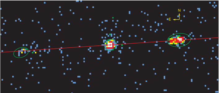
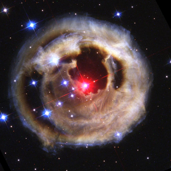
Figure 1: Upper panel: Two relativistic CBs emitted in opposite directions by the microquasar XTE J1550-564, seen in X-rays by Corbel et al. 2002. Lower panel: HST picture from 28 October 2002 of the glory, or light echo, of the stellar outburst of the red supergiant V3838 Monocerosis in early January 2002. The light echo was formed by scattering off dust shells from previous ejections (Bond et al. 2003).

The CBs of the CB model are inspired by the ones observed in quasar and microquasar emissions. One example of the latter is shown in the upper panel of Fig. (1), showing two opposite CBs emitted by the microquasar XTE J1550-564 (Kaaret et al. 2003). The winds and echoes of GRB-generating SNe are akin to those emitted and illuminated by some very massive stars. The light echo (or glory) of the stellar outburst of the red supergiant V3838 Monocerosis in early January 2002 is shown in the lower panel of Fig. (1), from Bond et al. (2003). In a sense all we are doing in this paper is to superimpose the two halves of Fig. (1), and to work out in detail what the consequences —based exclusively on Compton scattering— are.

The varied time structures of GRB $\gamma$-ray number-counts generally consist of fast rising and declining isolated or partially superimposed pulses. We show here that —in a CB model in which ICS of the wind’s ambient light is the dominant $\gamma$-ray-generating mechanism— the following observed properties of long-duration GRBs naturally follow (for the reader’s convenience, we also list here the equations and figures corresponding to the respective predictions):

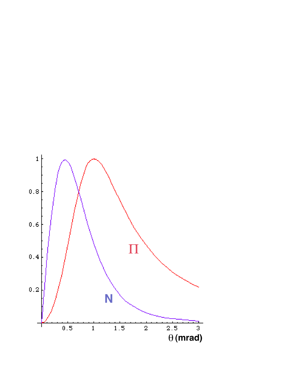
Figure 4: The predicted polarization $\Pi(\theta,\gamma)$ of Eq. (20) and the (arbitrarily normalized) rough expectation $dN_{GRB}/{d\theta\,dt}\propto\theta\,\delta^{3}$ for the rate of photons detected above a certain threshold, both as functions of $\theta$ (in mrad), at a typical $\gamma=10^{3}$. The observation of a GRB with a measured $\Pi=80\pm 20\%$ is seen to be very probable.

• The large polarization of the $\gamma$ rays (Coburn & Boggs 2003), Eq. (20) and Fig. (4).

• The characteristic energy $E={\cal{O}}(250)$ keV of the $\gamma$ rays (Preece et al. 2000; Amati et al. 2002), Eq. (21).

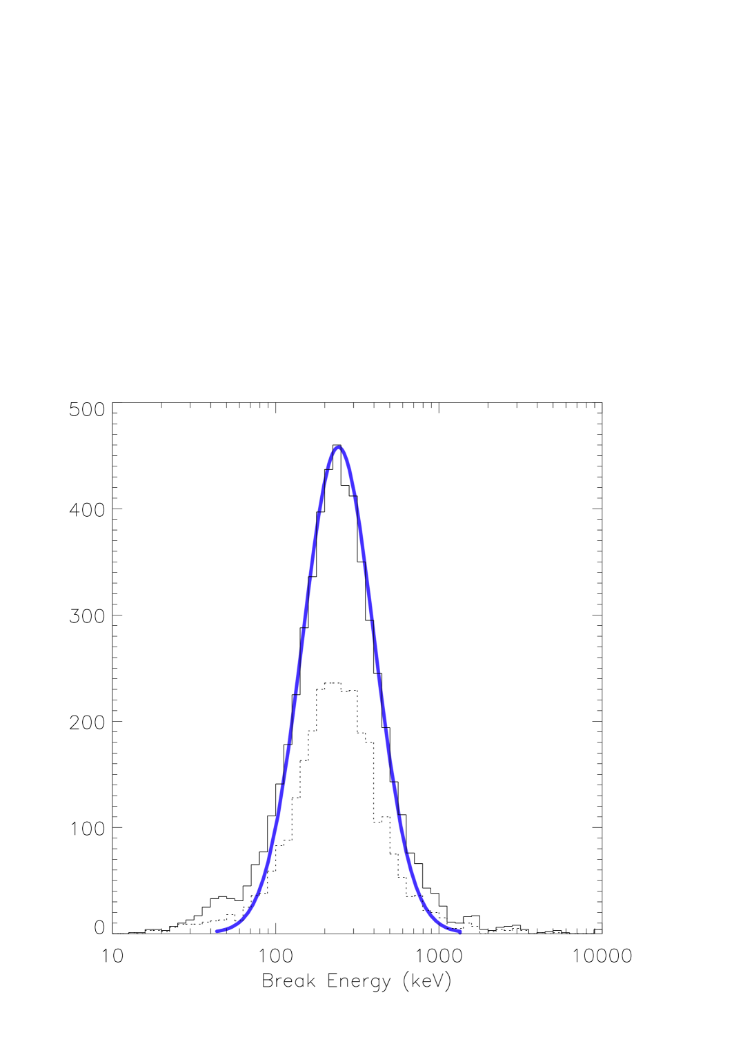
Figure 5: The break energy, or $E_{p}$ distribution of an ensemble of BATSE GRBs (Preece et al. 2000). The continuous line is borrowed from Fig. (6).

• The narrow distribution of the “peak” or “bend” energies of the GRB spectra (e.g. Preece et al. 2000), Eq. (21) and Fig. (5).

• The duration of the single pulses of GRBs: a median $\Delta t\sim 1/2$ s full width at half-maximum (McBreen et al. 2002), Eqs. (23) and (26).

• The characteristic (spherical equivalent) number of photons per pulse, $N_{\gamma}\sim 10^{59}$ on average, which, combined with the characteristic $\gamma$ energy, yields the average total (spherical equivalent) fluence of a GRB pulse: $\sim 10^{53}$ erg, Eqs. (13), (14), (33), (34).

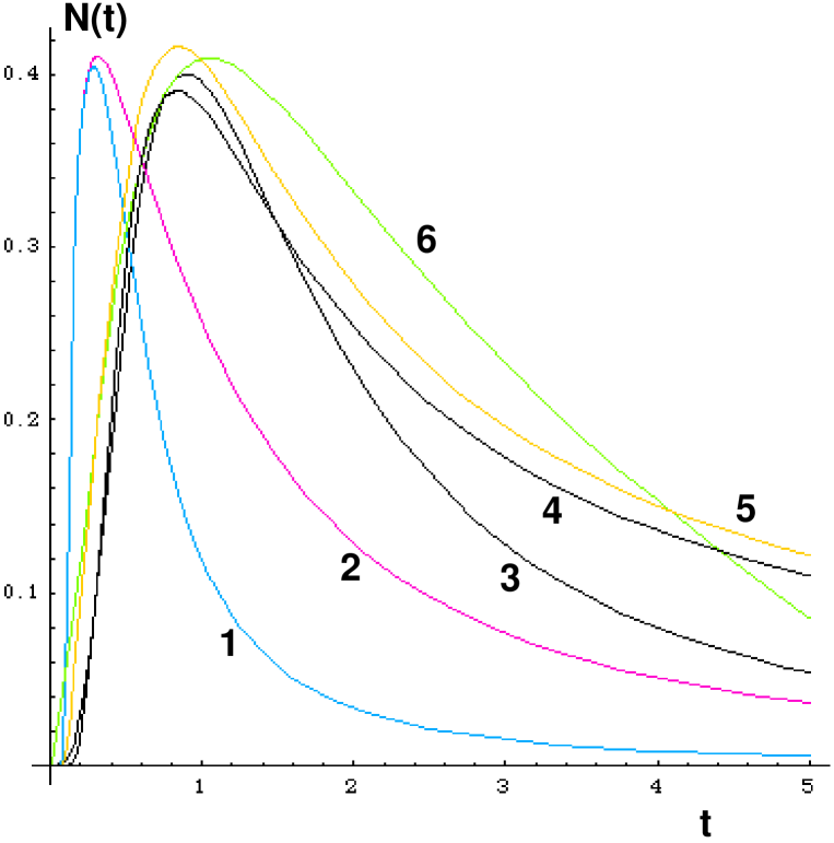
Figure 9: The shapes of GRB pulses for various CB geometries, described in the text.

• The general FRED pulse-shape: a very “fast rise” followed by a fast decay $N(t)\propto 1/t^{2}$, inaccurately called “exponential decay”, perhaps because FRPD is unpronounceable (Nemiroff et al. 1993, 1994; Link & Epstein 1996; McBreen et al. 2002), Eq. (38) and Fig. (9).

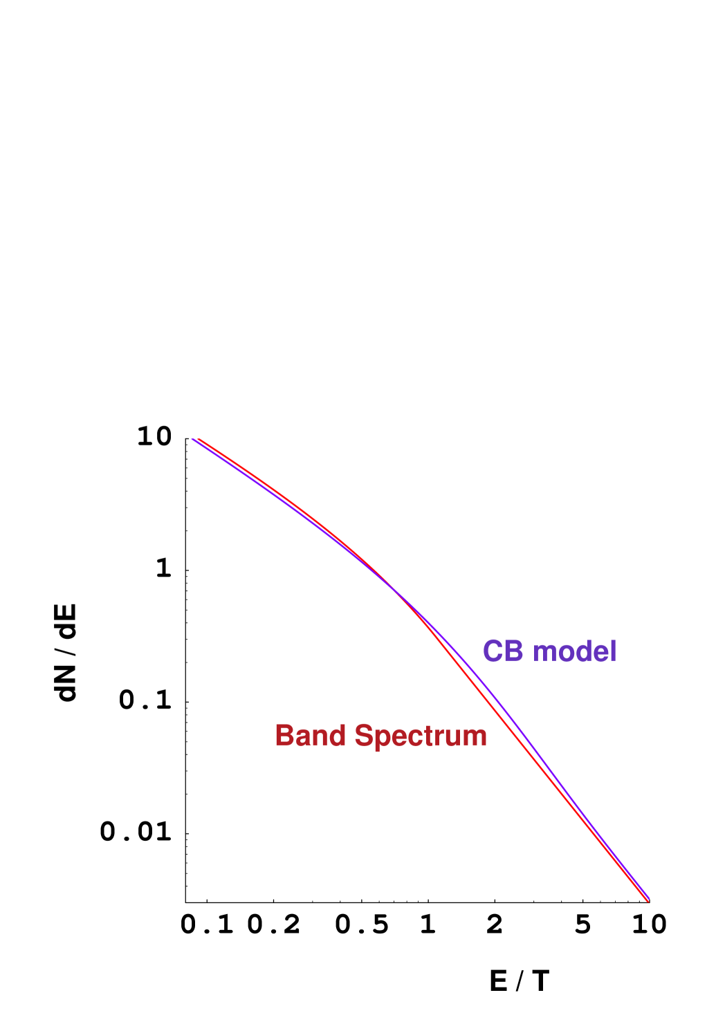
Figure 12: Two shapes of GRB spectra, the number of photons per energy interval $dN/dE$. One is the prediction of the CB model, Eq. (47). The other is the successful phenomenological Band spectrum of Eq. (48) (Band et al. 1993); $T$ stands for the bend energy in the Band’s case. Considering that the prediction is based exclusively on first principles, the agreement is rather satisfying.

• The $\gamma$-ray energy distribution, $dN/dE\sim E^{-\alpha}$, with, on average, $\alpha\sim 1$ exponentially evolving into $\alpha\sim 2.1$ and generally well fitted by the “Band function” (Band et al. 1993), our derived version of which is Eq. (47). The theoretical and Band spectra are compared in Fig. (12).

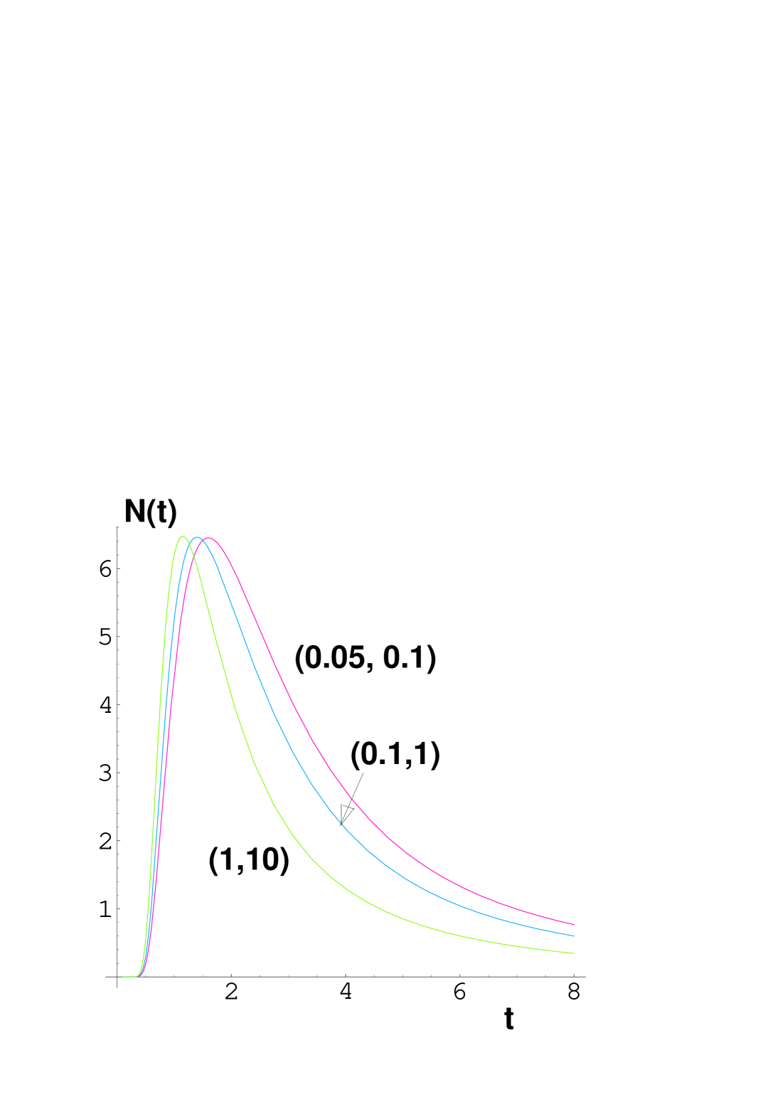
Figure 15: Pulse shapes (arbitrarily normalized for presentation) at three energy intervals, given in parenthesis in units of $T$ and corresponding to Eqs. (52, 53). The time is in units of $t_{tr}$.

• The time–energy correlation of the pulses: the pulse duration decreases like $\sim E^{-0.4}$ and peaks earlier the higher the energy interval (e.g. Fenimore et al. 1995; Norris et al. 1996; Ramirez-Ruiz & Fenimore 2000; Wu & Fenimore 2000); the spectrum gets softer as time elapses during a pulse (Golenetskii et al. 1983; Bhat et al. 1994), Eqs. (52) to (56) and Figs. (15) to (18).

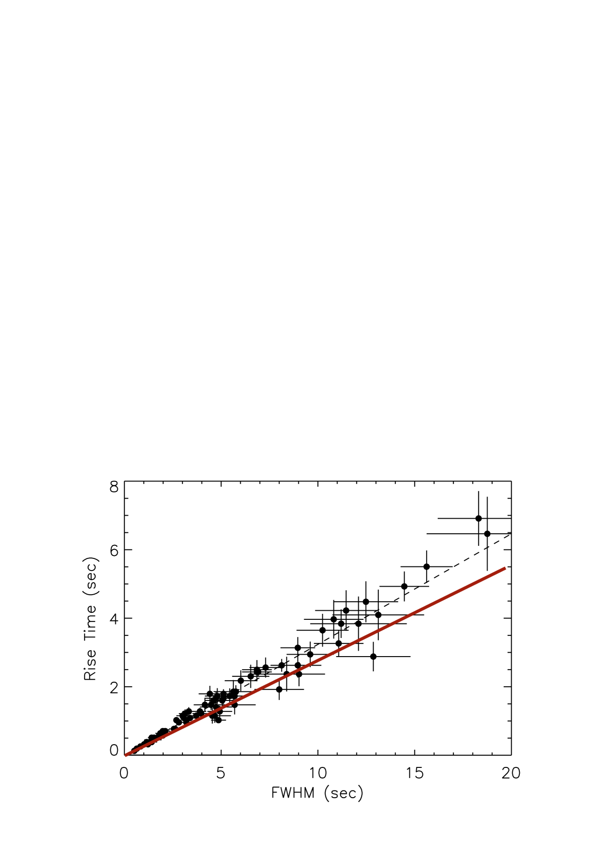
Figure 11: Rise-time from half-maximum to maximum versus full width at half-maximum of an ensemble of GRB single pulses (Kocevski et al. 2003). The data are from pulses of bright BATSE GRBs, the theoretical prediction (the continuous line) is from the naive pulse shape of Eq. (37). The dotted line is the best linear fit.

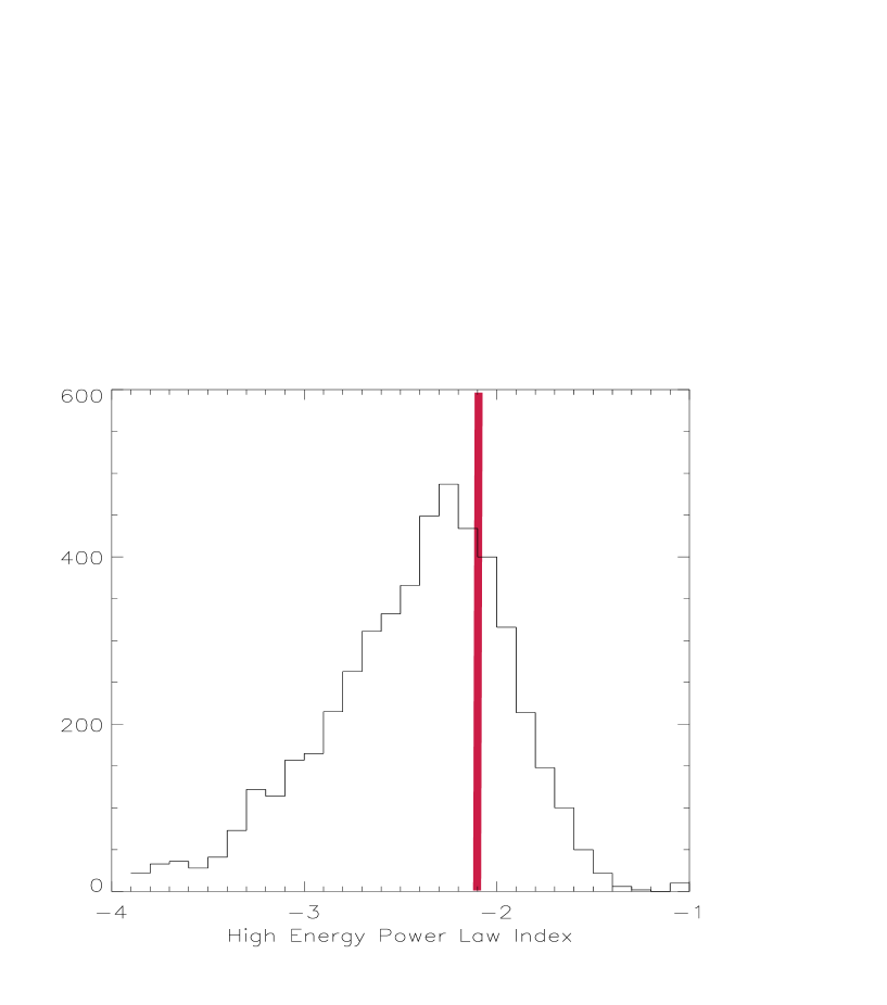
Figure 13: Upper panel: The observed distribution of the index $-\alpha$ of Eq. (47), compared with its central predicted value (the line). Lower panel: The same for the index $-\beta$. The data analysis is that of Preece et al. (2000) and, in the $\beta$ distribution. We have eliminated their bin at $\beta=4$, which contains events without a determined $\beta$. The prediction for the central $\alpha$-value does not depend on the adopted index of the accelerated electron distribution; the one for $\beta$ does. We interpret the events with $\beta>2.1$ as due in part to the effect of the energy cutoff of the knocked-on electrons, Eq. (40).

• Various correlations between pairs of the following observables: photon fluence, energy fluence, peak intensity and luminosity, photon energy at peak intensity or luminosity, and pulse duration (e.g. Mallozzi et al. 1995; Liang & Kargatis 1996; Crider et al. 1999; Lloyd, Petrosian & Mallozzi 2000; Ramirez-Ruiz & Fenimore 2000; McBreen et al. 2002; Kocevski et al. 2003), Eqs. (56) to (61) and Figs. (11,13) and (19) to (26).

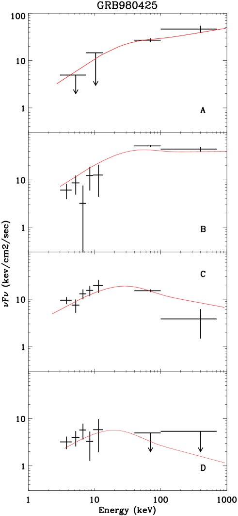
Figure 27: The distributions $\nu\,F_{\nu}\equiv E^{2}\,dN/dE$ of GRB 980425 in the time intervals (in seconds after the onset of the burst) A = (0,5), B = (5,10), C = (10,30) and D = (30,50), measured with Beppo-Sax by Frontera et al. (2000). The lines are not fits, but “descriptions” (with all parameters but $t_{c}$ at their reference values, and $\beta_{2}$ at the $\beta$ peak value, 2.3, as in Fig. (13) made using Eqs. (52, 53, 54, 55).

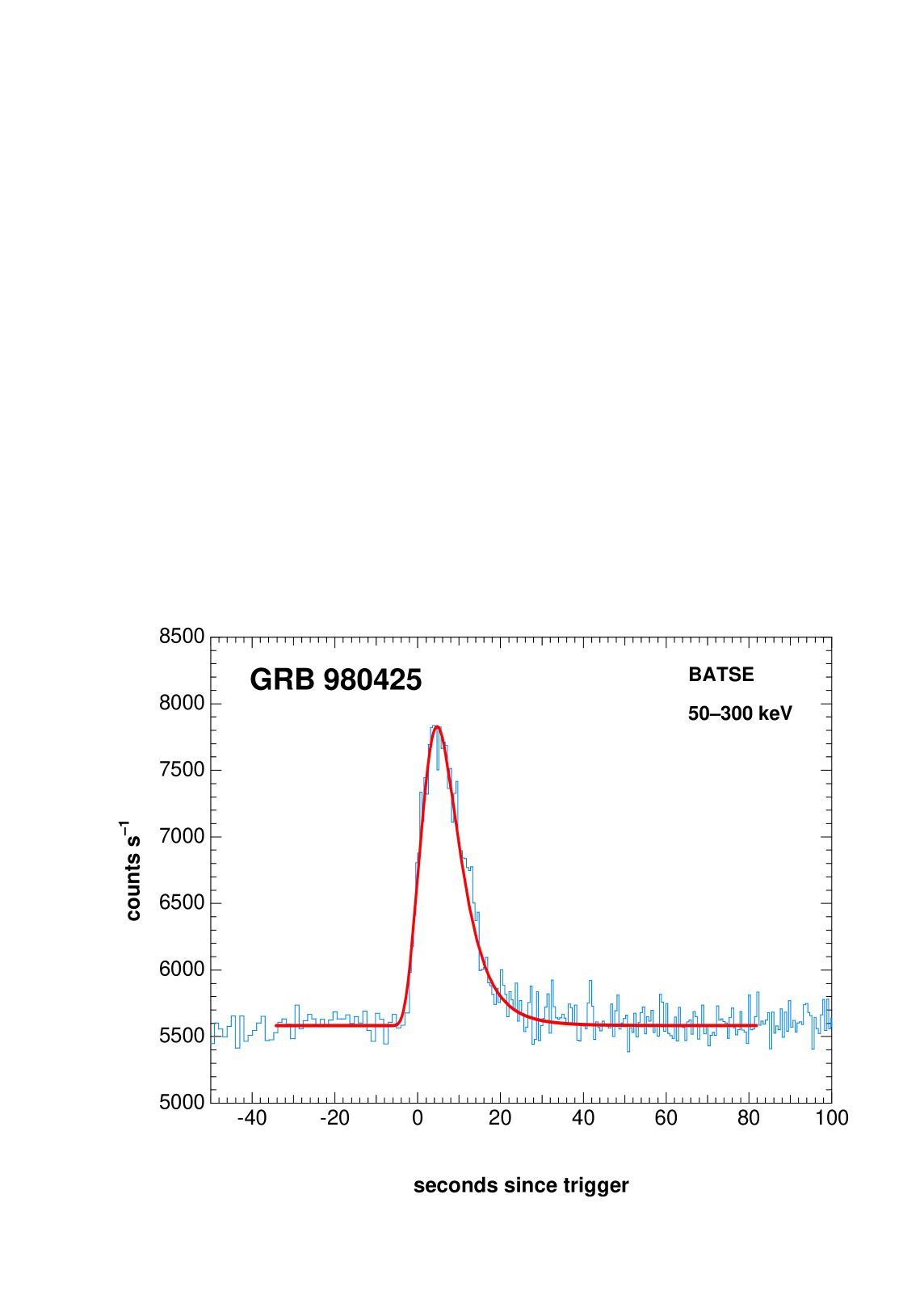
Figure 28: The single pulse in the light curve $dN/dt$ of GRB 980425, as seen by BATSE at energies in the 50–300 keV bracket (Kippen 1998) and its description in the CB model.

• The completion of the demonstration that both GRB 980425 and its associated SN1998bw were in no way exceptional, summarized by Figs. (27,28).

We have organized this paper in order of the increasing amount of algebra required to derive the results. But for the last two items, the ensuing order is that of the above list. By far the largest amount of algebra, but the one leading to one of our most detail-independent, —i.e. “first-principled”— results, is the one involved in the theoretical derivation of the Band spectrum.

For the sake of hypothetical readers not very familiar with the field, we also include various comparative discussions of the FB models and the CB model. Section 19 is a brief review of the FB-models’ results on the $\gamma$-rays of GRBs. Shocks are a fundamental building-block of the FB models, while in the CB model they play no role. The substance of the shells responsible GRBs is, in the FB models, an $e^{+}e^{-}$ plasma with a fine-tuned “baryon load”. The substance of CBs is ordinary matter. In Appendix I we review the observational situation regarding these two issues in the realm of the other relativistic jets observed in nature: the ejecta of quasars and microquasars. We devote Appendix II to a short commentary on GRB AGs —as described by the FB and CB models. But for the last item above, we have nothing new to add in this paper on the subject of the association of GRBs and SNe. But the question is important because —in the CB model— SNe are the progenitors of GRBs, and because —in the FB models— the GRB/SN association is gaining importance, subsequent to the discovery of the pair GRB 030329/SN2003dh (Stanek et al. 2003; Hjorth et al. 2003). We review very briefly this subject, within the CB model, in Section 4.4. The history of the idea and its observational support are summarized in Appendix III.

2 The “wind” environment of SNe

Two SNe play a particularly important role in this chapter: SN1987A, famous for its proximity to us and for the neutrinos its core-collapse emitted, and SN1998bw, famous for its association with GRB 980425, and also for its relative proximity.

Massive stars lose mass throughout their life in the form of slow and fast winds, and die in SN explosions. The ejected stellar material has been detected as circumstellar nebulae around Wolf–Rayet stars, luminous blue variables, and blue and red supergiants, such as V3838 Monocerosis, shown in the lower panel of Fig. (1). The ejections feed and compress the nebulae into dense shells, which are ionized by the UV fluxes emitted by the stars. Ionized circumstellar nebulae surrounding young supernova remnants have also been detected around Cas A, extending to a distance of $\sim 7$ pc (7’ at a distance of 3.4 pc) by Fesen, Becker & Blair (1987) and around SN1987A. The nebula of SN1987A, observed as a dust echo, ends in a patchy shell of radius 4.5 pc (Chevalier & Emmering 1989).

The mass-loss rate from SN progenitors intensifies in their late evolutionary stages, which are not fully understood, in particular shortly before the explosion (e.g. Podsiadlowski 1992; Chugai 1997a,b; Chu, Weis & Garnett 1999; Chevalier & Oishi 2003). The observations of very narrow P-Cygni profiles superposed on the broad emission H$\alpha$ and H$\beta$ lines of the SN ejecta in some young SN remnants —e.g. in SN1997ab (Salamanca et al. 1998), SN1997cy (Turatto et al. 2000), SN1998S (Fassia et al. 2001), SN1997eg (Salamanca, Terlevich & Tenorio-Tagle 2002), SN1994W (Chugai et al. 2003) and SN1995G (Chugai & Danziger 2003)— indicate very high wind particle-number densities, $n\sim 5\times 10^{7}$ cm^-3, at the distances of ${\cal{O}}(10^{16})$ cm of interest to the production of GRBs in the CB model. The measured $n$ declines roughly as $1/r^{2}$ and its corresponding “surface density” is

$$\rho\,r^{2}\sim 10^{16}\;{\rm g\;cm^{-1}}.$$ (1)

This “close-by” result is two orders of magnitude larger than the one observed for “canonical” winds of massive stars with a typical mass loss rate $\dot{M}\sim 10^{-4}\,M_{\odot}$, and a typical wind velocity $V\sim 100$ km s^-1, which yield $\rho\,r^{2}=\dot{M}/4\,\pi\,V\,\sim 5\times 10^{13}$ g cm^-1 at distances of ${\cal{O}}(10)$ pc (for a recent review, see Chevalier 2003), the ones relevant to the CB model predictions for GRB AGs (Dado et al. 2003e). This alterity of surface densities may be understood if the star’s $\dot{M}/V$ increases to a much higher value in the final stages of its pre-SN evolution. This intensified wind may blow continuously or in a series of ejection episodes, and may also be non-isotropic, as the one shown in Fig. (1) is. We will refer to the circumstellar matter distribution simply as the wind.

3 The ambient light around SNe

The wind environment of SNe may be ionized prior to the SN explosion by the light of the progenitor star, which becomes intense even at Extreme Ultraviolet (EUV) frequencies prior to the explosion (the recombination time at the densities characteristic of the wind is very long). Even if that prior ionization did not occur, the wind is ionized by the EUV flash from the SN explosion: the observations of SN1987A indicate that SNe shine briefly at EUV frequencies a few hours after their core collapses, when the blast wave —presumably produced by the “bounce” of the collapse, and re-energized by neutrino energy deposition— reaches the surface of the progenitor star (e.g. Arnett et al. 1989; Leibundgut 1995) and/or, presumably, when the jet of CBs is ejected.

The fast, transient and hard initial rise in luminosity has been observed only in SN1987A: the International Ultraviolet Explorer satellite, which began observations of this SN a day after its neutrino burst, detected a strong UV continuum with a colour temperature exceeding 14000 K, which declined to $\sim$ 5000 K within 20 days. The luminosity of the EUV flash is expected to exceed $10^{43}$ erg s^-1 over a good fraction of an hour (see, e.g. Arnett et al. 1989 for a review), which provides a sufficient number of photons to fully ionize a 10–20 $M_{\odot}$ wind environment. For the observed “close by” wind densities, the ionized wind is semitransparent at visible and UV frequencies: neither optically thin nor thick.

Subsequent to the early ionizing UV radiation, Compton scattering of the SN light in the ionized wind, line emission and thermal bremsstrahlung, result in a locally quasi-isotropic light environment within the wind. Since we are more interested in the light permeating the wind than in the emitted “echo” light seen from afar, we shall give a name to the former embedded light: the ambient light. Since the wind is semitransparent, the expectation is that the ambient light should have a thin-bremsstrahlung spectrum: $dn_{\gamma}(E)\sim exp(-E/T)/E$. The wind may be highly structured by non-uniform emission in both time and angle. But, in a quasi-stationary situation, the photon density of the ambient light must be:

$$n_{\gamma}(r)\approx{L_{SN}\over 4\,\pi r^{2}\,c\,E_{i}}\,,$$ (2)

where $E_{i}\sim 1$ eV is the typical energy of an ambient-light photon, and $L_{SN}$ is the SN’s luminosity at early times. This estimate, which corresponds to a flux $c\,n_{\gamma}$, is accurate for the net outward flux, but may be an underestimate of the total flux, though a slight one, since the wind is semitransparent.

The observed initial bolometric luminosity of SN1987A, uncorrected for extinction, was $L_{{}_{SN}}\sim 3\times 10^{41}$ erg s^-1; it declined by one magnitude within a day (Arnett et al. 1989). The explosion energy of SN1987A, estimated from the observed velocity of the ejected shell, was smaller than that estimated for SN1998bw by an order of magnitude. This may imply that in its early phase SN1998bw was also approximately ten times more luminous. Indeed, this estimate is consistent with the early time observations of SN1998bw, started on April 26.60 UT, 1998 (Galama et al. 1998), 0.7 days after its associated GRB was detected with Beppo-SAX (Soffitta et al. 1998; Pian et al. 2000) and by BATSE (Kippen et al. 1998) on April 25.90915 UT, 1998. The V-band and R-band light curves of SN1998bw showed a slow initial decline, or a “plateau”, after which they rose at a rate of 0.25 mag per day. This plateau may have been the late signature of the expected sharp initial peak in the light curve as the blast wave reached the surface of the progenitor star, but lack of early-time data prevented establishing its existence in the EUV and UBI bands. Assuming a Galactic foreground extinction, $Av=0.2$, in the direction of SN1987A, we estimate its (spherical equivalent) luminosity to be

$$L_{{}_{SN}}=5\times 10^{42}{\rm\;erg\;s^{-1}}.$$ (3)

We shall use this estimate of the initial luminosity of SN1998bw, our “standard candle” for GRB-generating SNe.

4 The cannonball model

In the CB model, long-duration GRBs and their AGs are produced in ordinary core-collapse supernovae by jets of CBs, made of ordinary atomic matter, and travelling with high Lorentz factors, $\gamma$. An accretion disk or torus is hypothesized to be produced around the newly formed compact object, either by stellar material originally close to the surface of the imploding core and left behind by the explosion-generating outgoing shock, or by more distant stellar matter falling back after its passage (De Rújula 1987). A CB is emitted, as observed in microquasars, when part of the accretion disk falls abruptly onto the compact object (e.g. Mirabel & Rodrigez 1999; Rodriguez & Mirabel 1999 and references therein).

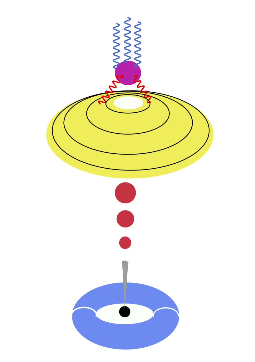
Figure 2: A fewer-kbyte version of Fig. (3) of Dar & De Rújula (2000a) showing an “artist’s view” (not to scale) of the CB model of GRBs and their afterglows. A core-collapse SN results in a compact object and a fast-rotating torus of non-ejected fallen-back material. Matter (not shown) abruptly accreting into the central object produces a narrowly collimated beam of CBs, of which only some of the “northern” ones are depicted. As these CBs move through the “ambient light” surrounding the star, they Compton up-scatter its photons to GRB energies.

The $\gamma$-rays of a single pulse in a GRB are produced as a CB coasts through the ambient light. An artist’s view of the CB model is given in Fig. (2). The electrons enclosed in the CB Compton up-scatter photons to GRB energies. Each pulse of a GRB corresponds to one CB. The timing sequence of emission of the successive individual pulses (or CBs) in a GRB reflects the chaotic accretion process and its properties are not predictable, but those of the single pulses are.

4.1 Times and energies

Let primed quantities refer to a CB’s rest system and unprimed ones to the observer’s system, a convention to which we shall adhere throughout this paper. Let $\theta$ be the angle between the line of sight and the CB’s velocity vector. Relative to their energy in the CB’s rest system, $E^{\prime}$, an observer at a redhift “distance” $z$, sees photons red-shifted by a factor $1+z$, and Lorentz-boosted, or blue-shifted, by a “Doppler” factor $\delta$:

$$E={\delta\over 1+z}\,E^{\prime},$$ (4)

$$\delta={1\over\gamma\,(1-\beta\,\cos\theta)}\approx{2\gamma\over 1+\gamma^{2}\,\theta^{2}}\;,$$ (5)

where the approximation is valid for $\gamma^{2}\gg 1$ and $\theta^{2}\ll 1$, the domain of interest here, for which $\beta\equiv 1/\sqrt{1-\gamma^{2}}\approx 1-1/(2\gamma^{2})$. The observed time intervals, $dt$, are related to those in a CB’s rest system, $dt^{\prime}$, by:

$$dt={1+z\over\delta}\,dt^{\prime},$$ (6)

where, this time, the factor $\delta$ is the literal (relativistic) Doppler factor of Doppler’s effect. The distance travelled by a CB in the SN rest frame during an observer time $dt$ is:

$$dx_{{}_{SN}}={\gamma\,\delta\over 1+z}\,c\,dt.$$ (7)

4.2 Angular distributions

Let $dN_{{}_{CB}}/d\Omega^{\prime}$ be the angular distribution of the time-integrated, total number of photons emitted by a CB in its rest system. Let $d{\cal{E}}^{\prime}_{{}_{CB}}/d\Omega^{\prime}$, likewise, be the distribution of the total energy carried by the photons. The relation between the observer’s viewing angle, $\theta$, and the same angle in the CB’s rest system, $\theta^{\prime}$, both relative to the CB’s direction of motion, is:

$$\cos\theta^{\prime}={\cos\theta-\beta\over 1-\beta\,\cos\theta}\,,$$ (8)

while $\phi^{\prime}=\phi$ for the azymuthal angles. The photon total number-fluence and energy-fluence measured by a cosmologically distant observer are, respectively:

$$f_{{}_{CB}}\equiv{dN^{obs}_{{}_{CB}}(\theta,\gamma)\over d\Omega}={(1+z)\,\delta^{2}\over D_{L}^{2}}\;{dN_{{}_{CB}}\over d\Omega^{\prime}}\,,$$ (9)

$$F_{{}_{CB}}\equiv{dF^{obs}_{{}_{CB}}(\theta,\gamma)\over d\Omega}={(1+z)\,\delta^{3}\over D_{L}^{2}}\;{d{\cal{E}}^{\prime}_{{}_{CB}}\over d\Omega^{\prime}}\,,$$ (10)

where $D_{L}(z)$ is the luminosity distance (7.12 Gpc at $z=1$, for the current cosmology with $\Omega=1$, $\Omega_{\Lambda}=0.7$ and $H=65$ km s^-1 Mpc^-1). For an isotropic emission in the CB rest frame, the total number of photons and the total energy fluence are, respectively:

$$f_{{}_{CB}}={(1+z)\,\delta^{2}\over 4\,\pi D_{L}^{2}}\;N^{T}_{{}_{CB}}\,,$$ (11)

$$F_{{}_{CB}}={(1+z)\,\delta^{3}\over 4\pi D_{L}^{2}}\;{\cal{E}}^{\prime}_{{}_{CB}}\,,$$ (12)

where $N^{T}_{{}_{CB}}$ is the total number of photons emitted by the CB, and ${\cal{E}}^{\prime}_{{}_{CB}}$ is their total energy in the CB’s rest frame (Shaviv & Dar 1995; Dar 1998). An observer who assumes —incorrectly, we contend— that the pulse is isotropic in the observer’s frame would infer much larger figures for the total number of photons and for the total energy in a GRB pulse:

$$N^{iso}_{{}_{CB}}={4\,\pi\,D_{L}^{2}\over 1+z}\,f_{{}_{CB}}=\delta^{2}\,N^{T}_{{}_{CB}}\,,$$ (13)

$${\cal{E}}^{iso}_{{}_{CB}}={4\,\pi\,D_{L}^{2}\over 1+z}\,F_{{}_{CB}}=\delta^{3}\,{\cal{E}}^{\prime}_{{}_{CB}}\,,$$ (14)

whereas the proper angular integration of Eqs. (11) and (12) yields $N_{{}_{CB}}$ for the total photon number and ${\cal{E}}_{{}_{CB}}=\gamma\,{\cal{E}}^{\prime}_{{}_{CB}}/(1+z)$ for their total energy in the observer’s frame.

4.3 Typical Lorentz factors and viewing angles

In our first analysis of GRBs in the CB model (Dar & De Rújula 2000a) we concluded that the typical Lorentz factors are $\gamma\sim 10^{3}$ and the typical viewing angles are $\theta\sim 1/\gamma$, so that $\delta\sim\gamma\sim 10^{3}$. This was corroborated by our systematic analysis of GRB AGs (Dado et al. 2002a, 2003a): we found that the fit values of $\gamma$ snuggly peak around 10³, while the $\theta$ distribution peaks around $\theta\sim 1/(2\gamma)$ and decreases fast thereafter, in good agreement with the expectation for the rate of photons detected above a certain threshold:

$${dN_{GRB}\over{d\theta\,dt}}\propto\theta\,\delta^{3}\;F(\delta),$$ (15)

where $F(\delta)$ is a complicated, slowly $\delta$-dependent function that depends on $z$, the geometry of the Universe and the case-by-case instrumental effects related to trigger and measuring efficiencies in various energy windows. That the distribution of $\theta$-values is narrow is the quintessential selection effect, induced by the very fast $\theta$-dependence in Eq. (15). The narrowness of the $\gamma$ distribution is physically significant, although some “tip-of-the-iceberg” effect no doubt plays a role. Three other parameters of interest here were constrained by our analysis of GRB AGs: the typical baryon (or electron) number of a CB, $N_{B}$; the total $\gamma$-ray energy emitted by a CB in its rest system, ${\cal{E}}^{\prime}_{{}_{CB}}$; and the CBs’ initial transverse velocity of expansion, $\beta_{s}\,c_{s}$, where $c_{s}=c/\sqrt{3}$ is the speed of sound in a relativistic plasma (Dado et al. 2002a, 2003a). These typical values are summarized in Table 1. In Table 2 we list the values of $\gamma$, $\theta$ and $\delta$ for the GRBs of known redshift whose AG we have analysed (Dado, Dar & De Rújula 2002a,b,c; 2003a,b,c,d,e,f).

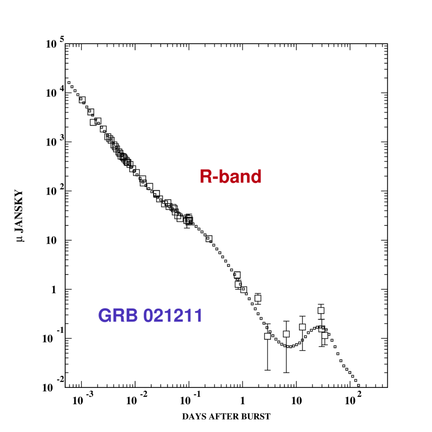
Figure 3: Observations of the R-band AG of GRB 021211, and their CB-model fit. The ISM density is a constant plus a “wind” contribution decreasing as the inverse square of the distance. The two density contributions are equal at $\bar{x}\simeq 1.2$ pc, a distance reached by the CBs in an observer’s time $\bar{t}\simeq 0.025$ days after burst (Dado et al. 2003e). The contribution of a SN1998bw-like SN at the GRB position is discernible as the bump at late times. The host galaxy’s contribution, which was also fitted, is subtracted in this plot.

Our confidence in the values of the parameters describing CBs and their circumstellar density profiles stems from the excellence of the description of AG light curves and spectra in the CB model. An example is given in Fig. (3), the R-band AG of GRB 021211 (Dado et al. 2003e). At a fixed optical frequency the prediction for the early AG’s fluence is simply $F_{\nu}\propto(n_{e})^{3/4}$, with $n_{e}$ the circumburst electron density, assumed to be a constant plus a wind contribution decreasing as the inverse square of the distance. This produces the observed early decline $\propto t^{-3/2}$ and the subsequent flattening at $t\sim 0.025$ d, at which point the two contributions to the density are equal and the CBs are at a distance $\bar{r}\simeq 1.2$ pc away from their parent SN. The fitted value of the wind’s grammage is $\rho\,r^{2}=(6.8\pm 0.5)\times 10^{13}$ g cm^-1, in agreement with the typical value $\rho\,r^{2}=5\times 10^{13}$ g cm^-1 for winds at that distance. Thereafter, as the CBs decelerate significantly, $F_{\nu}$ steepens. The late bump is the underlying SN, identical to SN1998bw except for the effects of redshift ($z=1.006$, in this case). The single expression for the AG fitting all of this evolution, as well as the wide-band spectrum, does an excellent job at describing the AGs and spectra of all other GRBs of known redshift, including GRB 980425 and its associated SN1998bw, neither of which is —in the CB model— exceptional. In Appendix II we give a brief comparison of the confrontation of the FB models and the CB model with the AG data.

4.4 The GRB/SN association in the CB model

In the CB model, by hypothesis, construction and demonstration, long-duration GRBs are made in core-collapse SN explosions (these SNe comprise all spectroscopic types, but Type Ia). What fraction of core-collapse SNe generate GRBs?

From a CB-model analysis of GRBs and their AGs, Dado, Dar & De Rújula (2002a,b,c; 2003a,b,c,d,e,f) determined that GRBs more distant than GRB 980425 are observable with past and current instruments only for $\theta\leq$ 2–3 mrad. With two CB jets per GRB, only a fraction

$$f\sim 2\,{\pi\,\theta^{2}\over 4\,\pi}\sim(2\;\rm{to}\;4.5)\times 10^{-6}$$ (16)

of SN-generated GRBs are observable. The SN rate in the visible Universe, $R_{SN}$, is proportional to the formation rate of massive stars, which is not very well known as a function of redshift (e.g. Madau et al. 1998). Using the observed SN rate in the local universe (e.g. Capellaro 2003), estimates cover the range:

$$R_{SN}\sim\rm{(1\;to\;10)\times 10^{8}\;yr^{-1}}.$$ (17)

About 25%–30% of all SNe in the local Universe are of Type Ia, and the rest are core-collapse SNe: 12%–15% of Type Ib/Ic and 55%–65% of Type II (Tammann, Loeffler & Schroeder 1994, van den Bergh & McClure 1994). If these rates were representative of a cosmic average, we would expect a rate of long-duration GRBs:

$$R_{GRB}\sim{\rm(0.7\;to\;0.75)}\;f\;R_{SN}\sim{\rm(140\;to\;3375)\;yr^{-1}.}$$ (18)

The value of $R_{GRB}$ inferred from BATSE observations (Fishman & Meegan 1995) is $\sim$ 500 to 700 yr^-1, compatible with the range in Eq. (18).

A comparison independent of the unknown star-formation rate at large $z$ yields a similar result: Schmidt (2001) has derived a luminosity function for GRBs of known redshift from which he estimated a local rate of long duration GRBs, $(2.5\pm 1.0)\times 10^{-10}\;{\rm Mpc^{-1}\,yr^{-1}}$ for the current cosmology. The local rate of core-collapse SNe is $(7.5\pm 3.8)\times 10^{-5}\;{\rm Mpc^{-1}\,yr^{-1}}$ (Cappelaro 2003). The ratio of these rates, $(3.3\pm 2.1)\times 10^{-6}$, is consistent with Eq. (16).

In view of the very large uncertainties, the fair conclusion is that the GRB rate is consistent with being equal, either to the total rate of core-collapse SNe, or to a fraction of it that may be as small as $\sim 1/4$. Within errors, it may also be that these statements apply to only the Type Ib and Ic subclasses. Spectroscopic information on many more SNe is needed before these issues can be decisively resolved.

5 The polarization of a GRB

In the CB’s system, because of the large value of $\gamma$, the bulk of the photons of the wind’s light (of energy $E_{i}={\cal{O}}(1)$ eV) are incident practically along the direction of relative motion, $\theta_{i}^{\prime}={\cal{O}}(1/\gamma)$. Their energy is $E^{\prime}_{i}={\cal{O}}(\gamma\,E_{i})\ll m_{e}\,c^{2}$, so that their Compton scattering cross section is in the low-energy “Thomson” limit. Let $\theta^{\prime}$ be the angle at which a photon is Compton scattered by a CB’s electron, related to the observer’s angle as in Eq. (8). The scattering linearly polarizes the outgoing photons in the direction perpendicular to the scattering plane by an amount (e.g. Rybicki & Lightman 1979):

$$\Pi(\theta^{\prime})\approx{1-\cos^{2}\theta^{\prime}\over 1+\cos^{2}\theta^{\prime}}.$$ (19)

Substitute Eq. (8) into Eq. (19) to obtain the value of the (Lorentz-invariant) linear polarization in the observer’s frame. In the large-$\gamma$ approximation, the result is:

$$\Pi(\theta,\gamma)\approx{2\;\theta^{2}\,\gamma^{2}\over 1+\theta^{4}\,\gamma^{4}},$$ (20)

which, for the probable viewing angles, $\theta\sim 1/\gamma$, is of ${\cal{O}}(100\%)$ (Shaviv & Dar 1995). This result is easy to understand: photons viewed at $\theta=1/\gamma$ had, according to Eq. (8), suffered a scattering of $\theta^{\prime}=90^{\rm o}$, which fully polarized them according to Eq. (19), as one may also recall from elementary electron-oscillator considerations.

The polarization $\Pi(\theta,\gamma)$ is a function of only the product $\theta\,\gamma$ and has a universal shape, but it is shown in Fig. (4) as a function of $\theta$ at $\gamma=10^{3}$, in order to compare it with the expected number, roughly $dN_{{}_{GRB}}\propto\theta\,[\delta(\theta,\gamma)]^{3}$, of GRBs detectable above a given flux threshold, as a function of $\theta$ at the same typical $\gamma$, see Eq. (15). Without further ado, the figure shows that it is very probable, in the CB model, to observe a GRB with a measured polarization $\Pi=80\pm 20\%$. To add some ado: the polarization of Eq. (20) exceeds 60% for $\sqrt{3}>\theta\,\gamma>1/\sqrt{3}$, which is the case for a third of the CBs listed in Table 2.

6 The energy of the $\gamma$ rays of a GRB

6.1 The typical energy

Let $E_{i}\sim 1$ eV be the typical photon energy of the wind’s ambient light. More precisely, $E_{i}$ is to be interpreted as the more sharply defined energy at which most of the energy of the ambient light resides (for a thermal or a thin thermal-bremsstrahlung spectrum that is the energy at which the distribution $E^{2}_{i}\,dn_{\gamma}/dE_{i}$ peaks). Let such a photon move with an angle $\theta_{i}$ relative to the direction of motion of the CB. Viewed from the CB’s system, the energy is $E^{\prime}_{i}=\gamma\,E_{i}\,(1+\beta\,\cos\theta_{i})$ and the incoming angle is $\theta_{i}^{\prime}\sim 0$. If the photon is deflected to an angle $\theta^{\prime}$ in the CB’s rest frame by Compton scattering, its energy changes very little, but in the SN rest frame its energy is boosted by the CB’s motion to $E\ =\gamma\,E_{i}\,(1+\beta\,\cos\theta_{i})\,(1+\beta\,\cos\theta^{\prime})$. Rewrite $\theta^{\prime}$ in terms of the observer’s angle $\theta$ with use of Eqs. (5) and (8), and take into account the cosmological redshift to obtain the measured energy of a GRB photon produced this way:

$$E\ = {\gamma\,\delta\over 1+z}\,(1+\beta\,\cos\theta_{i})\,E_{i}\,$$

$$= (500\;{\rm keV})\;\sigma\;(1+\beta\,\cos\theta_{i})\,{E_{i}\over 1\;\rm eV}$$

$$\sigma \equiv {\gamma\,\delta\over 10^{6}}\,{2\over 1+z}\;,$$ (21)

where we have normalized to an isotropic distribution of the ambient photons, $\langle\cos\theta_{i}\rangle=0$, and to the typical values of the parameters (the average $\sigma$ of the GRBs listed in Table 2 is 1.08). The result for $\langle(1+z)\,E\rangle$ is centred at $\sim 1$ MeV.

For typical parameters, the wind is semitransparent at the time a GRB pulse is emitted: its optical depth is $\sim 1/2$, as we shall see in detail in Section 7, Eqs. (23) and (25). For a non-transparent wind $\langle\cos\theta_{i}\rangle=0$, while for a transparent one, the ambient light photons would be radially directed away from the parent SN and $\langle\cos\theta_{i}\rangle=-1$. For the semitransparent typical case $\langle 1+\beta\,\cos\theta_{i}\rangle\sim 1/2$, and the central numerical prediction of Eq. (21) is 250 keV. This prediction precisely coincides with the observed median value of the peak energy (photon energy at peak $E^{2}\,dN/dE$) in GRBs, $\langle E_{p}\rangle\sim 250$ keV (e.g. Preece et al. 2000; Quilligan et al. 2002), or with the peak energy in the rest frame of the GRB’s progenitor: $E^{\prime}_{p}=0.5$ MeV, according to Amati et al. (2002), for GRBs of known $z$, for which $\langle z\rangle\sim 1$.

We conclude that GRBs are made of $\gamma$-rays of a few hundred keV energy because that is the typical energy to which ambient light is nearly-forward Compton up-scattered by electrons of $\gamma\sim 10^{3}$. The first attempt to explain GRB energies in this way was that by Shaviv & Dar (1995).

6.2 The energy distribution

One of the most puzzling facts about GRBs is the narrowness of the distribution of their typical energies, shown in Fig. (5) in terms of the “break energy”: the fitted energy at which their energy spectrum $dN/dE$ steepens, which is also, approximately, the energy $E_{p}$ at which $E^{2}\,dN/dE$ peaks (Band et al. 1993; Preece et al. 2000). In the CB model, this distribution is that of the factor $\sigma\,(1+\beta\,\cos\theta_{i})\,\epsilon_{i}$ in Eq. (21), with $\epsilon_{i}\equiv E_{i}/(1\;{\rm eV})$. We have no a-priori way of knowing what the distribution of values of $(1+\beta\,\cos\theta_{i})\,\epsilon_{i}$ is, but for the GRBs of known redshift whose AG we have fitted in the CB model, we know the $\sigma$ distribution.

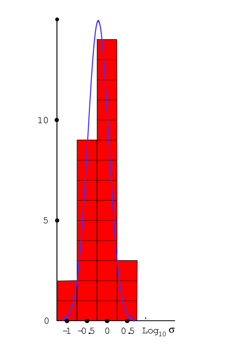
Figure 6: The distribution of the values of the quantity $\sigma$ defined in Eq. (21) and listed in Table 2. The line is a log-normal Kolmogorov-Smirnov fit to the unbinned $\sigma$ distribution.

In Table 2 we give the redshifts and fitted values of $\gamma$, $\delta$ and $\sigma$ for the quoted GRBs. The corresponding distribution in Log${}_{10}(\sigma)$ is shown in Fig. (6), where the continuous line is a (log-normal) fit. Due to the binning of the modest number of events shown in Fig. (6), the fit looks rough. But it is not. It was made with the known binning-independent Kolmogorov-Smirnov (KS) test, and its KS probability is a very comfortable 92%. With so little statistics on GRBs of known $z$, the fitted width of the Log${}_{10}(\sigma)$ distribution is only determined to $\sim 30$%. We have superimposed this KS fit on Fig. (5), showing it to be surprisingly compatible with the distribution of Log${}_{10}(E_{p})$. This leaves only little room ($<30$%) for a further (unknown) broadening due to the inevitable spread in $(1+\beta\,\cos\theta_{i})\,\epsilon_{i}$. In spite of this minor caveat, we consider the CB-model expectation for the narrow width of the $E_{p}$ distribution to be very satisfactorily consistent with the observations. For the central value of the theoretical distribution to agree with the observed one, as in Fig. (5), it must be that $\langle(1+\beta\,\cos\theta_{i})\,\epsilon_{i}\rangle\sim 0.5$, as we argued in the previous subsection.

7 The width in time of a GRB pulse

A CB is heated, while crossing the SN’s shell and prior wind, by hadronic collisions between the CB’s constituents and those of the circumburst material. This process stops as the expanding CB becomes transparent to these collisions. Let the ordinary matter of which the CB and the material it encounters are made be approximated as hydrogenic, and let the CB (in its rest frame) be approximated as a sphere of constant density. At $\gamma\sim 10^{3}$, the $pp$ cross section is dominantly inelastic and its value is $\sigma_{pp}\approx 40$ mb. The CB’s radius of collisional transparency is $R_{pp}\sim[3\,\sigma_{pp}\,N_{{}_{B}}/(4\pi)]^{1/2}$, or $\sim 10^{12}$ cm, for a CB’s baryon number $N_{{}_{B}}=10^{50}$. Since the CB’s initial internal radiation pressure is large, it should expand (in its rest frame) at a radial velocity $\beta_{s}\,c_{s}$ comparable to the speed of sound, in a relativistic plasma, $c_{s}=c/\sqrt{3}$.

Let $\sigma_{T}=0.665\times 10^{-24}$ cm^-2 be the Thomson cross section. A CB becomes transparent to its enclosed radiation when it reaches a radius:

$$R_{tr}\sim\sqrt{3\,\sigma_{T}\,N_{{}_{B}}\over 4\,\pi}\approx(4\times 10^{12}\,{\rm cm})\;\left({N_{{}_{B}}\over 10^{50}}\right)^{1\over 2}\,.$$ (22)

Seen by a cosmological observer, the time elapsed from the CB’s ejection to the point at which $R(t)=R_{tr}$ is:

$$t_{tr}=(0.46\,{\rm{s}})\;{1\over\beta_{s}}\;{10^{3}\over\delta}\;{1+z\over 2}\;\left({N_{{}_{B}}\over 10^{50}}\right)^{1\over 2}.$$ (23)

During this time the CB has moved a distance:

$$r_{tr}={\sqrt{3}\,\gamma\,R_{tr}\over\beta_{s}}\approx(6.9\times 10^{15}\,{\rm cm})\;{1\over\beta_{s}}\;{\gamma\over 10^{3}}\;\left({N_{{}_{B}}\over 10^{50}}\right)^{1\over 2}$$ (24)

away from its parent SN, a distance at which it is still embedded in the wind.

The electrons contained in a CB Compton up-scatter the ambient photons to the typical GRB energies of Eq. (21). But not all of them escape unscathed to become observable: they may be reabsorbed by the wind’s material. The probability that a GRB photon produced at a distance $r$ from the SN evades this fate, in a wind with a density profile $n_{e}\propto r^{-2}$, is $A(r)={\rm exp}[-(r^{w}_{tr}/r)^{2}]$ with $r^{w}_{tr}=\sigma_{T}\,\rho\,r^{2}/m_{p}$ the distance at which the remaining optical depth of the wind is unity. In the SN rest frame the “wind transparency time” is $r^{w}_{tr}/c$, and it corresponds to an observer’s time:

$$t^{w}_{tr}=(0.27\,{\rm s})\;{\rho\,r^{2}\over 10^{16}\,{\rm g\,cm}^{-1}}\;{1+z\over 2}\;{10^{6}\over\gamma\,\delta}\;,$$ (25)

coincidentally close —for the typical parameters— to the CB’s transparency time, $t_{tr}$.

Absorption in the wind affects the shape of a GRB pulse by a multiplicative factor $A(t)={\rm exp}[-(t^{w}_{tr}/t)^{2}]$, rising very fast from zero to unity. After the wind and the CB are both transparent, the number of photons per unit time in the pulse decreases with time as $(t_{tr}/t)^{2}$, simply reflecting the number density of the scattered ambient photons $n_{\gamma}\propto 1/r^{2}\propto 1/t^{2}$, as in Eq. (2). The net result —supported by our detailed study of the pulse shape in Section 9— is that the full width at half-maximum (FWHM) of a CB pulse is $t_{{}_{\rm FWHM}}\sim t_{tr}$ or, more precisely:

$$t_{{}_{\rm FWHM}}\approx 1.8\;t_{tr},$$ (26)

with $t_{tr}$ as in Eq. (23). For the standard CB parameters Eq. (26) yields $t_{{}_{\rm FWHM}}\approx 0.83$ s, in excellent agreement with the (median) observed result, $t_{{}_{\rm FWHM}}\approx 0.90$ s for photon energies above 20 keV. In the 110–325 keV energy band Lee, Bloom, & Petrosian (2000) report $t_{{}_{\rm FWHM}}\approx 0.68$ s and McBreen et al. (2002) obtain $t_{{}_{\rm FWHM}}\approx 0.58$ s (why pulses are narrower at higher energies is explained in Section 12).

8 The number of photons and the energy of a pulse

The number of ambient-light photons scattered by a CB into a particular observer’s angle can be computed explicitly, but it is a function of the CB’s geometry and the density distribution of electrons within the CB. Yet, to obtain a good estimate is fairly simple. The total number of ambient photons scattered by the CB up to its transparency time is:

$$N^{tk}\approx\pi\,\int^{R_{tr}}_{0}\,R^{2}\,n_{\gamma}\ dr\approx{L_{SN}\,\beta_{s}\,R_{tr}\over 4\,\sqrt{3}\,c\,\gamma\,E_{i}}\;,$$ (27)

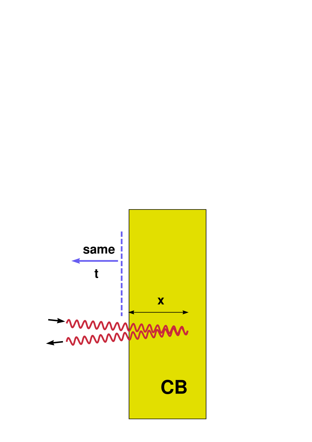
Figure 7: The “slab” CB geometry described in the text for the sake of illustration. Photons exiting the CB at the isochronous “same $t$” plane (the dashed line) may have suffered backward Compton scattering at various depths, $x$, corresponding to different times of entry of the incoming photon into the CB.

where we have used $R=R_{tr}\,(t/t_{tr})=R_{tr}\,(r/r_{tr})$ and Eqs. (2,22,24). The fraction of these photons that is observable depends on the relative values of the wind and CB absorption coefficients, which are comparable, according to Eqs. (23) and (25). It also depends on geometry: consider the likely case $\theta\sim 1/\gamma$ (scattering at right angles in the CB’s rest system, $\theta^{\prime}=\pi/2$) in two very extreme geometries. Within a longitudinally thin, slab-shaped CB, such as the one shown in Fig. (7), photons scattered onto that direction would all reinteract, and be degraded to lower energies by adiabatic cooling. A thin rocket-like CB, contrarywise, would let most of the photons scattered at right angles escape unscathed.

The total number of photons scattered after the CB becomes optically thin to Compton scattering, similarly calculated, is:

$$N^{tn}_{T}\approx\sigma_{T}\,N_{{}_{B}}\int_{R_{tr}}^{\infty}\,n_{\gamma}\ dr\approx{L_{SN}\,\beta_{s}\,R_{tr}\over 3\,\sqrt{3}\,c\,\gamma\,E_{i}}\;.$$ (28)

Around $t=t_{tr}$, photons have a roughly 50–50 chance of not being scattered a second time within the optically thinning CB. The total number of scattered photons is somewhere between $N^{tn}/2$ and $N^{tn}/2$ plus a small fraction of $N^{tk}=3\,N^{tn}/4$, so that $N^{tot}\simeq N^{tn}/2$. For a given angle of observation, the result is modulated by the relatively weak angular-dependent factor $G(\theta)$ in the Thomson scattering cross section:

$$G(\theta^{\prime})=1+\cos^{2}\theta^{\prime}$$ (29)

$${d\sigma\over d\Omega^{\prime}}={3\,\sigma_{{}_{T}}\over 16\,\pi}\,G(\theta^{\prime})\approx{3\,\sigma_{{}_{T}}\over 16\,\pi}\;{2\,(1+\theta^{4}\,\gamma^{4})\over(1+\theta^{2}\,\gamma^{2})^{2}}\,,$$ (30)

where in Eq. (30) we used Eq. (8) to express $G$ in the observer’s frame. The angular distribution of the number of scattered ambient photons and of their total energy in the CB’s rest system are:

$${dN_{{}_{CB}}\over d\Omega^{\prime}}\approx{3\,G\over 16\,\pi}\,N^{tot}\approx{G\,L_{{}_{SN}}\,\beta_{s}\,R_{tr}\over 32\,\sqrt{3}\,\pi\,c\,\gamma\,E_{i}}\,,$$ (31)

$${d{\cal{E}}^{\prime}_{{}_{CB}}\over d\Omega^{\prime}}\approx\gamma\,E_{i}\,{dN_{{}_{CB}}\over d\Omega^{\prime}}\approx{G\,L_{{}_{SN}}\,\beta_{s}\,R_{tr}\over 32\,\sqrt{3}\,\pi\,c}\,.$$ (32)

The total number of scattered photons is:

$$N_{CB} = \int d\Omega^{\prime}\,{dN_{{}_{CB}}\over d\Omega^{\prime}}$$ (33)

$$\approx (5\times 10^{52})\,\left({L_{{}_{SN}}\over 5\times 10^{42}\,{\rm erg}}\right)\,\left({1\,{\rm eV}\over E_{i}}\right)\,\left({N_{{}_{B}}\over 10^{50}}\right)^{1\over 2}\,\left(10^{3}\over\gamma\right)\,\beta_{s}\,,$$

and the equivalent spherical photon emission that follows from Eq. (13) is $\sim 10^{6}$ times larger. The energy emitted by a CB in its rest frame in the form of scattered ambient photons, is:

$${\cal{E}}^{\prime}_{CB} = \int d\Omega^{\prime}\,{d{\cal{E}}^{\prime}_{{}_{CB}}\over d\Omega^{\prime}}$$ (34)

$$\approx (0.8\times 10^{44}\,{\rm erg})\;\left({L_{{}_{SN}}\over 5\times 10^{42}\,{\rm erg}}\right)\,\left({N_{{}_{B}}\over 10^{50}}\right)^{1\over 2}\;\beta_{s},$$

and the equivalent spherical energy that follows from Eq. (14) is $\sim 10^{9}$ times larger, i.e. ${\cal{E}}^{iso}\sim 0.8\times 10^{53}$ erg. The average ${\cal{E}}^{iso}$ of the GRBs with known redshift that were measured by BeppoSAX is $\sim 6\times 10^{53}$ erg (Amati et al. 2002). There are 6 pulses on the average in a single GRB (Quilligan et al. 2002), yielding $\sim 10^{53}$ erg mean pulse-energy, in agreement with the expectation.

We have fitted to the CB model the AGs of all GRBs of known redshift (Dado et al. 2002a,b,c; 2003a,b,c,d,e,f; Dado et al. in preparation) and extracted the parameters $\theta$ and (the initial) $\gamma$ for all of them, in the approximation that the AG is dominated by one CB, or a collection of similar ones. From these analyses we extracted, using Eqs. (5) and (10), the value of ${\cal{E}}^{\prime}_{{}_{CB}}$ for each GRB, in an approximation in which the weak angular dependence of the Thomson cross section was neglected (an excellent approximation around the most probable observation angles $\theta\sim 1/\gamma$, for which $G\approx 1$). The remarkable result was that the values of ${\cal{E}}^{\prime}_{{}_{CB}}$ span a very narrow rage: from 0.6 to 2.1 times 10⁴⁴ erg, see Fig. (41) of Dado et al. (2002a). Also to be remarked is how close these results are to the simple prediction of Eq. (34).

It is at first sight surprising that the parameters in Eq. (34) conspire to give a rather narrow range of ${\cal{E}}^{\prime}_{{}_{CB}}$ values. Yet, it is not unreasonable that $\beta_{s}$ be narrowly distributed around 1, the expectation for an expanding relativistic plasma. The baryon number dependence is only via a square root. But why should $L_{{}_{SN}}$ be in a narrow range? Besides SN1998bw, there is only one other SN for which the early $L_{{}_{SN}}$ was measured: SN1987A. Both SNe have the same ratio of $L_{{}_{SN}}$ to peak optical luminosity. It is quite conceivable that core-collapse SNe be much less varied than the observations seem to indicate: much of the variability could be due to the different observer’s angles relative to the jet axis of bipolar CB emission, so that these SNe would be standard torches, rather than standard, spherically-emitting candles.

9 The shape of a GRB pulse

9.1 Smooth pulse shapes

Let us first discuss the shape of a pulse for which the quantities defined in Eqs. (23) and (25) satisfy $t_{tr}\gg t^{w}_{tr}$, so that $\gamma$-ray absorption in the wind plays no significant role. We shall also simplify the discussion to a manageable level by working out the result for photons scattered only once within the CB, more collisions “adiabatically” degrade the photon energy because of the CB’s expansion.

The shape of a GRB pulse depends, albeit quite moderately, on the CB’s geometry. To illustrate this fact, we have worked out the result for various geometries and observation angles. The simplest case to present is an unrealistically extreme but “pedagogical” geometry: a CB consisting of a slab that is much larger in the direction transverse to its motion than in the direction parallel to it, as in Fig. (7). Consider photons suffering backward scattering: exiting the CB in the direction opposite to the incoming one. Photons reaching an observer at a fixed time may originate from different depths into the slab at which they interacted: they have different times of entry into the CB. To lighten the notation let $t^{\prime}$ be temporarily umprimed and let time be measured in units of $t_{tr}$, so that $t=1$ is transparency time. Let also the unit of distance be such that $c=1$. Let $n_{{}_{CB}}(t)\propto 1/t^{3}$ be the time-varying CB’s density, approximated as uniform within the CB. As in Fig. (7) the photons interact at the various depths $(t-x)$, and they must escape absorption during their trip to that point and back. The pulse’s photon number per unit time is then:

$${dN\over dt} \approx K\int_{0}^{Up(t)}\!n_{{}_{CB}}(t-x)\,dx\;e^{-\sigma_{T}\;\int^{t}_{t-2\,x}\,n_{{}_{CB}}(t^{\prime})\,dt^{\prime}}$$ (35)

$$\propto \int_{0}^{Up(t)}{dx\over(t-x)^{3}}\;exp\left[{1\over 2\,t^{2}}-{1\over 2(t-2\,x)^{2}}\right]\;,$$

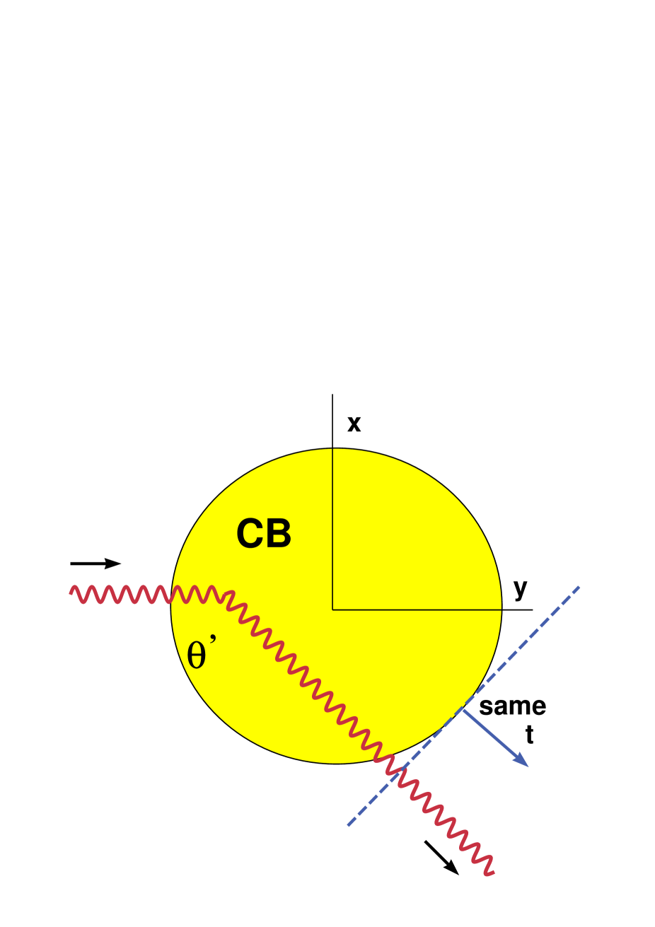
Figure 8: The spherical CB geometry described in the text. Photons exiting the CB at the isochronous “same $t$” plane (the dashed line) may have suffered Compton scattering at a given angle ($\theta^{\prime}$ in the CB’s rest frame) at various positions within the sphere. We have not attempted to draw this figure in its full 3-D detail.

where $Up(t)={\rm min}[t/2,\,R(t)]$, $K\equiv\pi\,R^{2}\,n_{\gamma}\,d\sigma_{T}(\pi)/d\cos\theta$, and we have used the fact that $R^{2}\propto t^{2}$ and $n_{\gamma}\propto t^{-2}$. We have also simplified the result by use of Eqs. (2), (22) and (24). The case of a spherical CB seen at any given angle, shown in Fig. (8), is a trivial but very tedious 3-D generalization of Eq. (35).

The pulse shapes for various geometries and scattering angles in the CB system are shown in Fig. (9), in which time is measured in units of the observer’s transparency time: $t_{tr}$ in Eq. (23). The curves labelled 1 and 2 are for the slab geometry of Eq. (35), with $\beta_{s}=1/5$ and 1 for the expansion velocities, respectively. The result for a spherical CB, also at a backward scattering angle, and with $R(t)$ fixed ($\beta_{s}=0$), is labelled 6. The result labelled 5 is for the same geometry and $\beta_{s}=1/5$. The other two pulse shapes are for a sphere seen at right angles in the CB rest system (an observer’s $\theta=1/\gamma$), 4 is for $\beta_{s}=1/5$ and 3 for $\beta_{s}=1$. The difference between the shape of the slab light curves and the others is only apparent, an increase of $t_{tr}$ by a factor of 2 in the slab pulse shapes makes them resemble the others. Except for the fixed-radius case, the large-$t$ pulse shapes and their normalization are the ones implied by Eq. (28), to wit:

$${dN\over dt}\to c\,\sigma_{T}\,G\,N_{{}_{B}}\,n_{\gamma}\propto 1/t^{2}\;,$$ (36)

with $G$ as defined in Eq. (30). A decline $\sim 1/t^{2}$ is the mean observed late-time dependence of GRB pulses (Giblin et al. 2002).

To a rather good approximation, all the expanding-CB pulses in Fig. (9) have shapes that resemble that of the very simple function:

$${dN\over dt}=exp\left(-\,{1\over t^{2}}\right)\,\left[1-exp\left(-\,{1\over t^{2}}\right)\right],$$ (37)

with time measured in units of $t_{tr}$.

Several complications may affect this result. First, pulses are observed in certain energy intervals, and their shapes depend on these, as we discuss in detail in Section 12. Second, absorption in the wind, if the condition $t_{tr}\gg t^{w}_{tr}$ is reversed, modifies Eq. (37) into $exp(-(t^{w}_{tr}/t)^{2})\,[1-exp\{-(t_{tr}/t)^{2})\}]$. A further complication is that the “effective number” of Compton up-scattered photons is modulated, as is their final energy in Eq. (21), by a factor $1+\beta\,\cos\theta_{i}$, which decreases as $1/r^{2}$ at distances large enough for the wind to be quite transparent. A pulse’s late rate of decline may therefore evolve in some cases from $1/t^{2}$ to $1/t^{4}$. We embody all of these complications in the following approximate form of a pulse:

$${dN\over dt}=exp\left[-\left({t_{1}\over t}\right)^{m}\right]\,\left\{1-exp\left[-\left({t_{2}\over t}\right)^{n}\right]\right\}\,.$$ (38)

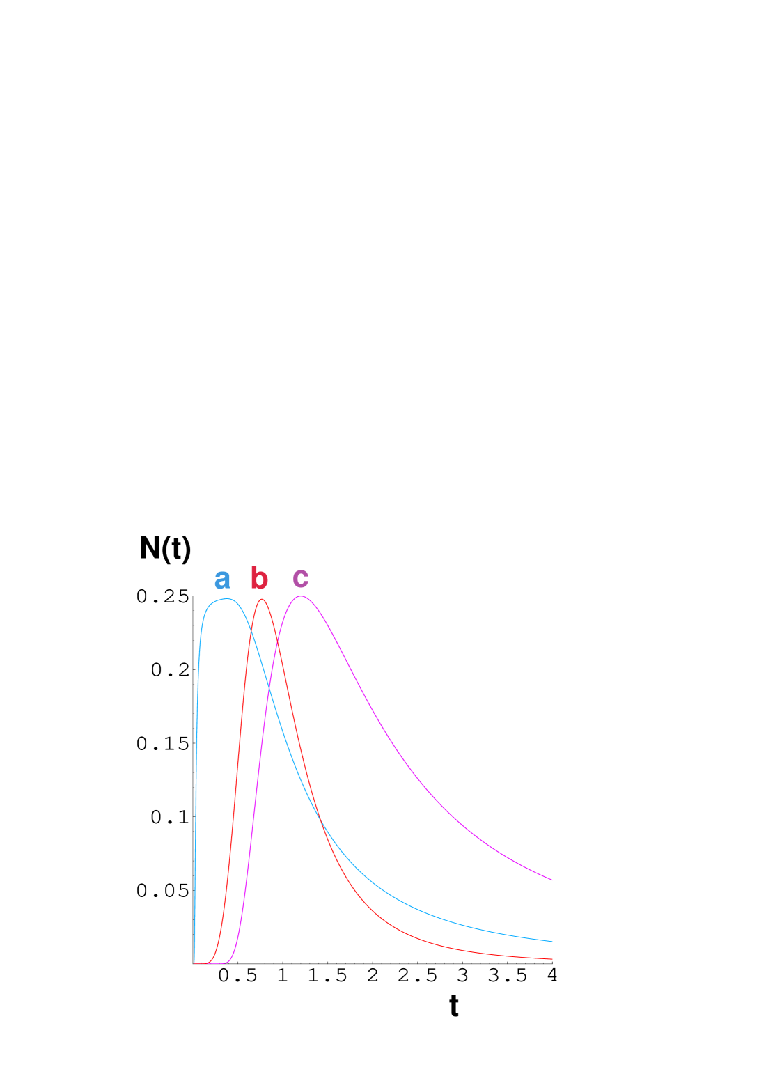
Figure 10: Three shapes of GRB pulses, as described by Eq. (38). a) is for $t_{1}=0.03\,t_{2}$ and $m=n=2$. b) has $t_{1}=t_{2}$, $m=2$ and $n=4$. c) is the “typical” CB-model pulse shape with $t_{1}=t_{2}$ and $m=n=2$. These shapes describe GRB pulses integrated over energy.

Even the most naive pulse shape with $m=n=2$, $t_{1}=t_{2}$, shown in Fig. (10), does a very good job at describing individual “FRED” shapes as well as results averaged over all observed GRB shapes. For example, for this pulse shape, the ratio of the rise-time from half-maximum to maximum to the total width at half-maximum is, $\simeq 0.27$, while the observed result, reproduced in Fig. (11) is $\sim 0.3$ (Kocevski et al. 2003). Also shown in Fig. (10) are a very fast-rise case with $t_{1}=0.03\,t_{2}$, $m=n=2$, and a fast-decline case with $t_{1}=t_{2}$, $m=2$ and $n=4$.

9.2 The fast variability of GRB light curves

It is often claimed that GRBs have “variability” at the few millisecond level (e.g. Walker, Shaefer & Fenimore 2000 and references therein). Yet, the Fourier transform $P(\omega)$ of GRB light curves has very little power at $\omega=100$ Hz and above, compared with the power at $\omega\sim 1$ Hz —the frequency at which $P(\omega)$ “bends”— reflecting the fact that the structure of most GRBs is dominated by rather smooth pulses of $\sim 1$ s width, and not by much narrower features. The fraction of GRBs with significant variability much faster than 1 Hz must be small, as reflected by the Fourier properties of GRB ensembles (Shaviv & Dar 1995; Beloborodov et al. 2000). In order to extricate a putative short-time variability from the data, methods more sophisticated than mere Fourier transforms appear to be necessary.

Two common dictums in high energy physics are: “Do not trust results coming from the edge of your distributions” and “If you need statistics —rather than your naked eye— to prove your discovery, you have not made one”. These wisecracks make us a tad uneasy about the subject of this subsection.

In a paper where they studied 20 GRBs, Walker et al. (2000) found that two short-duration GRBs had spikes of a few ms duration. In a wavelet analysis of the ensemble, which included 5 GRBs with short ($<2$ s) duration, they concluded that the majority had “spikes or flickers with rise times shorter than 4 ms in the first $\sim 1$ s of their light curves”.

At first sight, the CB model cannot accommodate such results, since the shape of the pulses in Fig. (9) is dominated by retardation effects: it takes a time of ${\cal{O}}(t)$ for a photon to enter the CB, scatter within it, and exit in a given direction to be observed at time $t$. This means that short pulse substructure is, as allegedly observed, more likely at early times. But, how can it be produced? A non-uniform density distribution within a CB is not the answer, for the volume integration at fixed $t$ would erase its details. But suppose that the density distribution, quite reasonably, is significantly peaked towards the centre of a (roughly spherical) CB. At the transparency time corresponding to the average density, then, the core of the CB may be quite non-transparent, while the rest is transparent. Consider a number-density inhomogeneity in the ambient light, such as would be produced by an over-density inhomogeneity in the wind, as the ones pictured in Fig. (1). Seen by the CB in its rest system, the inhomogeneity is longitudinally foreshortened by a factor $\gamma$. Its photons are likely to scatter the central overdensity. This would produce a “spike” whose duration is of the order of the light-crossing time of the core overdensity, which may be much smaller than that of the CB as a whole. It is even likely that the ambient-light temperature within the overdensity be enhanced, which would make the spikes’ spectrum harder, as claimed by Walker et al. (2000).

In the FB models the fast variability plays an important role, the width of the colliding $e^{+}e^{-}$ shells is adjusted to produce it (e.g. Waxman 2003a).

10 Shockless acceleration

In Dado et al. 2002a, we argued that the electrons entering a CB from the external medium would undergo acceleration by their successive deflections in its enclosed chaotic and turbulently moving magnetic field. Subsequently, there have been illuminating numerical studies of this process (Frederiksen et al. 2003). These authors have investigated what happens when a collisionless plasma of ions and electrons impinges at large $\gamma$ on a similar plasma at rest. The trajectory of each particle is governed by the Lorentz force that the ensemble of all other particles exert on it, whose $\vec{E}$ and $\vec{B}$ fields are determined by Maxwell’s equations. An infinitesimal seed magnetic field suffices to separate the trajectories of the different-charge particles, creating an instability leading to moving electric fields (that is, extra magnetic fields). The process induces a turbulent flow and a turbulent magnetic field that is carried in with the incoming particles at $v\sim c$. The particles are accelerated extremely fast by their interactions with these fields to a spectrum hardening with energy to a power law,

$${dn\over dE}\propto E^{-p},\;\;\;\;\;p\sim 2.2.$$ (39)

In this acceleration and magnetic-field-generating process there are no shocks: no surfaces discontinuously separating two domains and, consequently, no “shock acceleration” by successive crossings of the shock, the mechanism allegedly responsible for particle acceleration in the FB models, as discussed in Appendix I. The moving “front” of the incoming particles within the bath of the target ones does not leave on its wake neither a kinetic nor a true thermal distribution. In front of the front nothing happens.

These numerical studies are approximations, in that the statistics are limited, the ratio $m_{e}/m_{p}$ is not as small as the observed one, the transverse boundary conditions are periodic, as opposed to self-regulatory, and radiative processes are ignored. Yet, none of their input ingredients —special relativity, Maxwell’s equations and the Lorentz force— is potentially dubious. That is why we have refrained from calling these studies simulations.

In the bulk of a non-transparent CB, the shockless acceleration process would be quenched by Coulomb interactions with the enclosed photon bath. However, in the outer transparent part of the CB (that at $t\sim t_{tr}$ becomes the whole object), the acceleration process does take place. It is from this region that ambient photons entering the CB are scattered out; they are thus subject to Coulomb collisions with accelerated electrons, not only unaccelerated ones.

While a CB is not yet fully transparent to the strong interactions of the wind’s hadrons that penetrate it, there is another mechanism endowing it with a high-energy electron constituency. The entering hadrons lose energy mainly by Coulomb collisions with the CB’s electrons, which lead to electromagnetic showers initiated by the knocked-on electrons. In the CB’s rest system, a nucleus of charge $z$ and Lorentz factor $\gamma$ gives rise to knocked-on electrons (or “$\delta$-rays”) with Lorentz factors up to $\gamma^{\prime}_{e,max}\approx 2\,\gamma^{2}$. In a CB of density $n_{{}_{CB}}$, the number of electrons scattered to a Lorentz factor $\gamma^{\prime}_{e}$ is:

$${d^{2}N_{e}\over d\gamma^{\prime}_{e}\,dt} \approx 2\,\pi\,r_{e}^{2}\,n_{{}_{CB}}\,c\,z^{2}\;{F(\gamma^{\prime}_{e})\over(\gamma^{\prime}_{e})^{2}}\,,$$

$$F(\gamma^{\prime}_{e}) \approx 1-{\gamma^{\prime}_{e}\over\gamma^{\prime}_{e,max}}\,,$$ (40)

where $r_{e}$ is the classical electron radius. For electrons with Lorentz factors considerably smaller than $\gamma^{\prime}_{e,max}$, the shape of the knocked-on electron distribution of Eq. (40) is $\approx dn/dE\propto E^{-2}$, very close to that of the accelerated electrons in Eq. (39), for which $p\sim 2.2$. For photons scattered by knocked-on electrons closer to the cutoff $\gamma^{\prime}_{e,max}$, the effective value of $p$ may be greater than 2.2.

11 The GRB spectrum

The “final” energy distribution $dN/dE$ of the $\gamma$ rays in a GRB pulse is that of the “initial” ambient-light photons, $dN/dE_{i}$, uplifted by ICS with the electrons of a moving CB. Let the initial ambient-light number density be approximated as a thin thermal bremsstrahlung spectrum of temperature $T_{i}$:

$${dN\over dE_{i}}\propto{1\over E_{i}}\;e^{-E_{i}/T_{i}}\,.$$ (41)

The energy (or Lorentz factor) distribution of the electrons within the CB has two components. One corresponds to the bulk of the CB’s electrons, comoving with the CB and having non-relativistic motions in its rest frame. The other corresponds to the electrons that have been accelerated to an approximate power-law distribution. The total electron-number distribution as a function of their Lorentz factor $\gamma_{e}$ is, in the CB’s rest frame:

$${dN\over d\gamma_{e}^{\prime}}\propto\delta(\gamma_{e}^{\prime}-1)+{b^{\prime}\over(\gamma_{e}^{\prime})^{{\tilde{p}}}}\;,$$ (42)

where $b^{\prime}$ is a constant that we do not attempt to determine a-priori. The “cooling time” of these accelerated electrons to Compton scattering off the photons enclosed in a semi-transparent CB is of the same order as the Coulomb transparency time of the CB. Therefore, we expect $\tilde{p}$ to evolve in such a time from $\tilde{p}=p\simeq 2.2$, the index expected in the absence of cooling, to $\tilde{p}=p+1\simeq 3.2$, the index expected for a completely “cooled” spectrum (once again, the contribution of knocked-on electrons may result in an evolution to $\tilde{p}>3.2$). In this section we discuss the GRB spectrum at fixed $\tilde{p}$, the effects of its evolution are discussed in the next section.

11.1 ICS convolutions, an approximate treatment

The exact convolution of $dN/dE_{i}$ and $dN/d\gamma_{e}$ via Compton scattering involves the angular distribution of the latter, as well as the angular distributions of the target photons and the accelerated electrons within the CB. Even in the approximation in which these distributions are isotropic (in their different respective frames), this convolution is fairly complex. We discuss it in some of its gory detail in the next subsection. Here we just outline the derivation of the final result, the various steps being quite intuitive. The gist of the simplification is that all of the distributions being convoluted are very broad, and it is consequently an extremely good approximation to substitute a (well chosen) subset of these distributions (essentially the ICS one) by their averages. This fact is familiar in the study of ICS (Rybicki & Lightman 1979) and considerably simplifies the discussion.

Let us first study ICS by the electrons at rest in the CB. The discussion is simplest in the SN rest frame, in which the electrons are comoving with the CB at a common Lorentz factor $\gamma_{e}=\gamma$, so that their distribution is $dN/d\gamma_{e}=\delta(\gamma_{e}-\gamma)$. In this frame, the average energy of a Compton up-scattered electron —viewed in the final state at an angle $\theta$, corresponding to a Doppler boost $\delta$— is $\bar{E}(E_{i})=(4/3)\,\gamma\,\delta\,E_{i}\,\langle 1+\cos\theta_{i}\rangle$. Substituting this average for the corresponding distribution, we obtain:

$${dN\over dE} \propto \int d\gamma_{e}\,dE_{i}\;\delta(\gamma_{e}-\gamma)\;{e^{-E_{i}/T}\over E_{i}}\;\delta\left[E-\bar{E}(E_{i})\right]$$ (43)

$$\propto {1\over E}\;e^{-E/T}\;,$$

where, including the effect of cosmological redshift,

$$T\equiv{4\over 3}\;T_{i}\;{\gamma\;\delta\over 1+z}\;\,\langle 1+\cos\theta_{i}\rangle.$$ (44)

The interpretation of Eqs. (43) and (44) is obvious: the target ambient-photon distribution is simply boosted by ICS on the comoving electrons to a similar distribution at a much higher energy scale.

Inverse Compton scattering by the power-law-distributed electrons in Eq. (42) is simplest to discuss in the CB’s rest frame. In it, the initial ambient photons are beamed towards the CB in a narrow cone of opening $\sim 1/\gamma$. They have an energy distribution akin to that of Eq. (41), with $T_{i}\to\gamma\,T_{i}$, that is, $dN/dE_{i}^{\prime}\propto exp[-E_{i}^{\prime}/(\gamma\,T_{i})]/E_{i}^{\prime}$. They collide with electrons of various $\gamma_{e}$, moving isotropically in this frame, so that the collisions are at various angles and the relative velocity of the “beams” is also varying. We prove in the next subsection that —once again because of the smoothing effect of convoluting broad distributions— the brutal “approximation” of considering only head-on collisions is actually a very good one, it simply changes a little the energy scale of the $E^{\prime}$ distribution. In this approximation, the average energy of a scattered photon is $\bar{E}^{\prime}(E^{\prime}_{i})=(4/3)\,\gamma_{e}^{2}\,E_{i}^{\prime}\,\langle 1+\cos\theta_{i}\rangle$, and:

$${dN\over dE^{\prime}} \propto \int d\gamma_{e}\,dE^{\prime}_{i}\;{1\over(\gamma_{e})^{{\tilde{p}}}}\;{e^{-E_{i}^{\prime}/(\gamma\,T_{i})}\over E_{i}^{\prime}}\;\delta\left[E^{\prime}-\bar{E}^{\prime}(E_{i}^{\prime})\right]$$ (45)

$$\propto {1\over E^{\prime}}\;\int_{1}^{\infty}{d\gamma_{e}\over(\gamma_{e})^{{\tilde{p}}}}\;exp\left[-{3\,E^{\prime}\over 4\,\gamma\,T_{i}\,\langle 1+\cos\theta_{i}\rangle}\;{1\over\gamma_{e}^{2}}\right].$$

To express this result in terms of the observer’s GRB energies, we must replace in the above expression $T_{i}\to\delta\,T_{i}/(1+z)$. The $\gamma_{e}$ integral in Eq. (45), for any ${\tilde{p}}>1$, is an incomplete $\Gamma$ function which, for ${\tilde{p}}\sim 3$ and to an excellent approximation, is:

$$\int_{1}^{\infty}{d\gamma_{e}\over(\gamma_{e})^{{\tilde{p}}}}\;exp\left[-{a\over\gamma_{e}^{2}}\right]\approx(1-e^{-a})\;a^{-{{\tilde{p}}-1\over 2}}\,,$$ (46)

an exact result for ${\tilde{p}}=3$.

We may now replace Eq. (46) into Eq. (45) and add the result to that of Eq. (43) to obtain the complete spectrum of the observed $\gamma$ rays in a GRB:

$${dN\over dE} \propto \left({T\over E}\right)^{\alpha}\;e^{-E/T}+b\;(1-e^{-E/T})\;{\left(T\over E\right)}^{\beta}$$

$$\alpha = 1\;;\;\;\;\;\;\;\;\;\beta={{\tilde{p}}+1\over 2}\approx 2.1\,,$$ (47)

with $T$ as in Eq. (44), and $b$ a constant that we have made dimensionless by rescaling the two contributions to $dN/dE$ by appropriate powers of $T$. The quoted $\alpha$ and $\beta$ are “preferred” values, because the power index of the accelerated plus knocked-on electrons may not be exactly ${\tilde{p}}=3.2$ (which affects $\beta$); the ambient-light distribution may not be exactly “thin-thermal” and its effective temperature $T_{i}$ may vary along the CB’s trajectory (which affects both $\alpha$ and $\beta$). Notice that the shape of the spectrum in Eq. (47) is independent of the CB’s expansion rate, its baryon number, its geometry and its density profile. Moreover, its derivation rests only on observations of the properties of the surroundings of exploding stars, Coulomb scattering, and an input electron-distribution extracted from numerical studies also based only on “first principles”.

The predicted $dN/dE$ of Eq. (47) bears a striking resemblance to the Band distribution traditionally used to describe GRB energy spectra (e.g. Band et al. 1993: Preece et al. 2000 for an analysis of BATSE data, Amati et al. 2002 for BeppoSAX data, and Barraud et al. 2003 for HETE II data):

$${dN\over dE} = \left({E_{ref}\over E}\right)^{\alpha}\;e^{-E/E_{0}}\;\;\;\;{\rm for}\;\;E\leq(\beta-\alpha)\,E_{0}\,;$$ (48)

$$= \left[{(\beta-\alpha)\,E_{0}\over E_{ref}}\right]^{(\beta-\alpha)}\;e^{(\beta-\alpha)}\;\left({E_{ref}\over E}\right)^{\beta}\;\;\;\;{\rm otherwise.}$$

In this Band spectrum, $E_{0}$ plays the role of $T$ in Eq. (47). The energy at which $E^{2}\,dN/dE$ is maximal is often called the peak energy, $E_{p}$. Its value is $E_{p}\simeq E_{0}$, an exact result for $\alpha=1$, $\beta=2$.

The similarity of the prediction of Eq. (47) and the consuetudinary spectrum of Eq. (48) is demonstrated in Fig.(12), where we have plotted the two distributions for $\alpha=1$, $\beta=2.1$, and $T$, $b$, $E_{0}$ and $E_{ref}$ all set to unity. One cannot tell which curve is which! Considering that the prediction is based on first principles, the agreement is rather satisfying.

The distributions of values of $\alpha$ and $\beta$ extracted from fits to the GRB data (e.g. Preece et al. 2000; Amati et al. 2002; Quilligan et al. 2002) peak close to the values expected in the CB model $\alpha\approx 1$, $\beta\approx 2.1$, as we show in Fig. (13). The result for $\alpha$, which does dot depend on an adopted power for the spectrum of accelerated electrons, is more satisfactory than the result for $\beta$, which does. In particular, the events for which $\beta>2.1$ may reflect, as we have discussed, the cutoff energy of the knocked-on electrons in Eq. (40).

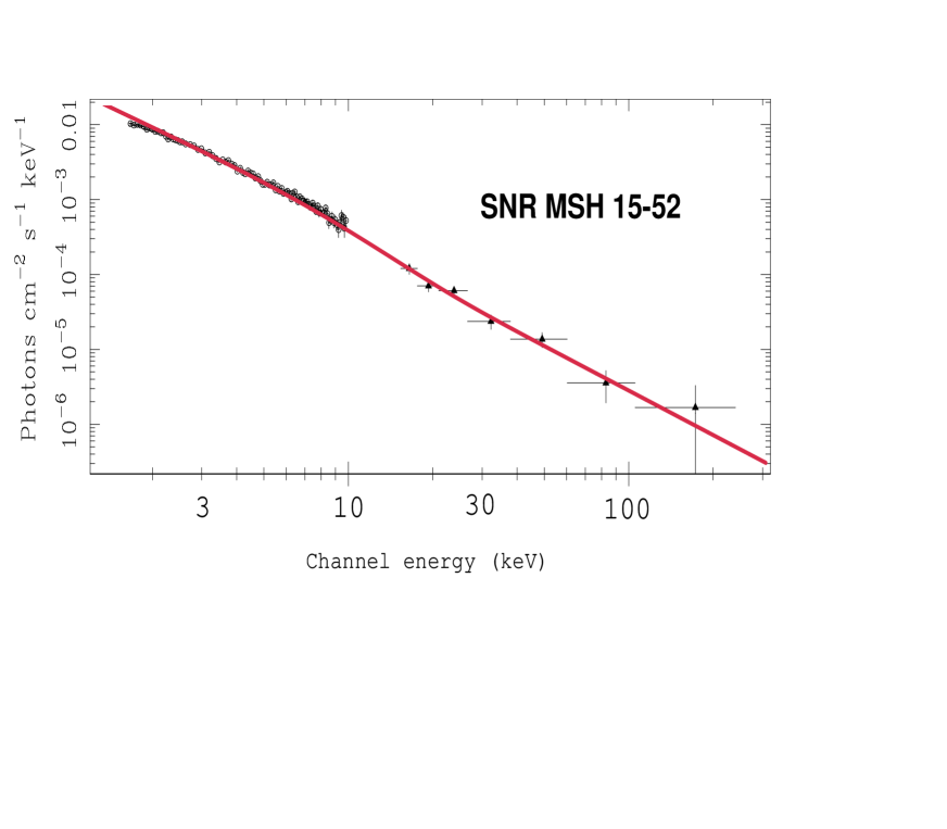
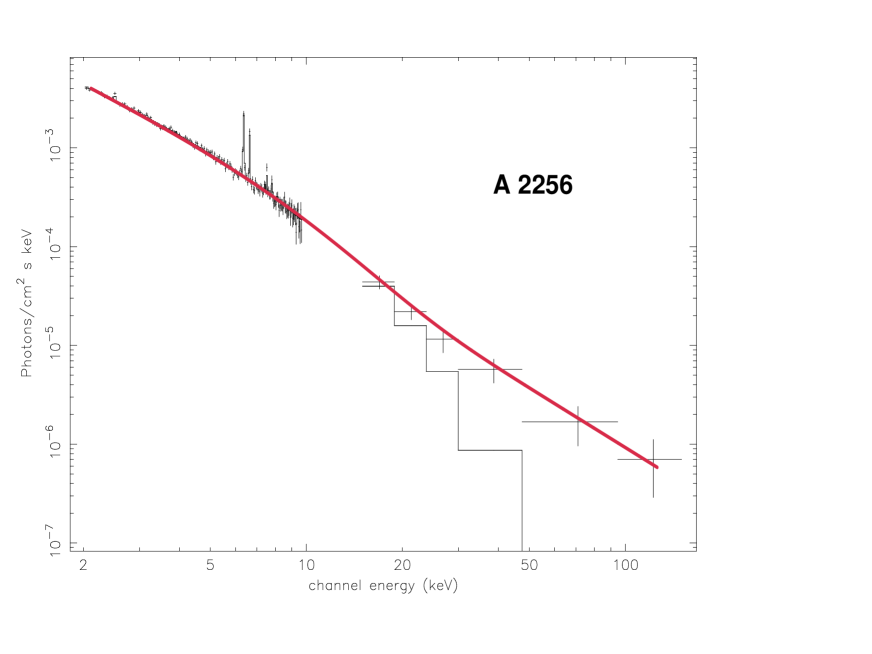
Figure 14: Two figures from Colafancesco, Dar & De Rújula (2003). Upper panel: The thick (red) line is a “$\chi$-by-eye” fit of Eq. (47) to the thin thermal bremsstrahlung emission from the SN remnant SNR MSH 15-52. The data and figure are from Mineo et al. (2001). Lower panel: The same for the cluster A2256. The data and figure are from Fusco-Femiano et al. (2000). The thin (black) line is their binned, purely thermal extrapolation.

In the CB model, spectra with the shape given by Eq. (47) are not the exclusivity of GRBs. All plasmas subject to an intense flux of cosmic rays (such as a CB in its rest system) have analogous spectra. Two examples are given in Fig. (14), borrowed from Colafrancesco, Dar & De Rújula (2003). One of them is that of the SN remnant SNR MSH 15-52, the other that of the galaxy cluster A2256.

11.2 ICS convolutions, a sketch of the exact treatment

Consider an electron belonging to the “thermal” (i.e. unaccelerated) constituency of a CB, travelling, in the SN rest frame, with a Lorentz factor $\gamma_{e}=\gamma$, and Compton scattering ambient-light photons with the energy distribution of Eq. (41) and an approximately isotropic initial directional distribution (the inclusion of a non-trivial angular dependence with $\langle\cos\theta_{i}\rangle\neq 0$ can be made along identical lines). The exact calculation of the energy distribution of the photons scattered by the electrons —which is also the exact calculation of the relativistic Sunayev–Zeldovich effect— can be paraphrased from Cohen, De Rújula and Glashow (1998). Let $d^{2}N(E,E_{i})/dE_{i}\,dE$ denote the number of photons transferred by one electron from the energy interval $dE_{i}$ to the interval $dE$. Define:

$${d^{2}N(E,E_{i})\over dE_{i}\,dE}={d^{2}N(E,E_{i})\over dE\,dn}\;{dn(E_{i})\over dE_{i}}\;.$$ (49)

The function $d^{2}N(E,E_{i})/dE\,dn$ may be regarded as the spectral distribution of struk photons of energy $E$ produced as the energetic electron Compton-scatters the light of an isotropic, monochromatic photon gas of unit density and energy $E_{i}$.

Let $d\Omega_{i}(\theta_{i},\phi_{i})$ be the differential solid angle about the initial photon direction, and $v_{i}$ be the relative speed of the colliding particles. We choose to measure angles relative to the total momentum direction of the colliding particles. The function $d^{2}N/dE\,dn$ is obtained by averaging the differential transition rate over target photon directions:

$${d^{2}N\over dE\,dn}=\int\frac{d\Omega_{i}}{4\pi}\,v_{i}\,\frac{d\sigma(E_{i},E)}{dE\,d\Omega_{i}}\ ,$$ (50)

where we have neglected the tiny effect of stimulated emission.

Since $\gamma\,T_{\gamma}\ll m_{e}$, the Thomson limit applies: the exact expression for ${d\sigma/dE\,d\Omega_{i}}$ is relatively simple. After a little algebra, the integrand in Eq. (50) can be rewritten as:

$$v_{i}\,\frac{d\sigma}{dE}=\frac{3\,\sigma_{T}}{16\,\mu^{4}\,\beta^{5}\,\gamma^{10}\,E_{i}}\biggl{\{}\mu^{2}\gamma^{2}\,(1+2\gamma^{2})(1-2\gamma^{2}\mu)+(3-4\gamma^{2})\mu^{4}\gamma^{4}+4\mu^{6}\gamma^{6}$$

$$+r\,(r-2\,\mu\,\gamma^{2})\,\left[3-6\,\mu\,\gamma^{2}+\mu^{2}\gamma^{2}\,\left(1+2\,\gamma^{2}\right)\right]\biggr{\}}\,\Theta\left(\frac{\mu}{1+\beta}<r<\frac{\mu}{1-\beta}\right)\ ,$$

where $r\equiv E/E_{i}$ and $\mu\equiv 1-\beta\cos\theta_{i}$.

Carrying out the integrations in Eq. (50) gives a relatively simple result for $d^{2}N/dE\,dn$, a function of only two variables: $E_{i}$ and $E$. This can then be introduced into Eq. (49), and integrated in initial photon energies $E_{i}$. The overall result of this exercise is extremely well approximated by the simple and intuitive expression in Eq. (43).

The detailed discussion of ICS by the accelerated electrons is entirely analogous to the above, though somewhat lengthier, not because of the need to integrate over their energy distribution, but mainly because of the extra angular sum over electron directions, akin to that in Eq. (50). Rather than giving the complete discussion, we outline the reason why the angular sum “does not matter”, in the same sense in which the detailed angular sum in Eq. (50) insignificantly affected the result of Eq. (43), in which this average was skirted in an apparently cavalier fashion.

Let an accelerated electron, in the CB rest system, be moving with a Lorentz factor $\gamma_{e}$ and velocity $\beta_{e}$, at an angle $\alpha$ relative to the direction of the ambient photons, travelling in this system practically along $\alpha=\pi$ (we are using units in which $c=1$). The relative $e\,\gamma$ velocity is $v_{i}=(1+\beta_{e}^{2}+2\,\beta_{e}\,\cos\alpha)^{1/2}$. The average energy of the photons struk by the electrons, upscattered from an energy $E_{i}^{\prime}$ , is $E^{\prime}\sim(4/3)\gamma_{e}^{2}\,E_{i}^{\prime}\,(1+\beta_{e}\,\cos\alpha)$. The net result of taking the distribution in $\alpha$ into account is to modify Eq. (46) to

$$\int_{1}^{\infty}{d\gamma_{e}\over(\gamma_{e})^{{\tilde{p}}}}\int^{1}_{-1}d\cos\alpha\;v_{i}\;exp\left[-{a\over\gamma_{e}^{2}\,(1+\beta_{e}\,\cos\alpha)}\right].$$ (51)

This function, to an excellent approximation, has the same shape as that of the r.h.s. of Eq.(46), simply rescaled by $a\to 0.8a$, tantamount to a 20% modification of $T$ in Eq. (44). In an entirely analogous fashion one can demonstrate that, to an excellent approximation, a deviation from an assumed isotropic ambient-light bath ($\langle\cos\theta_{i}\rangle=0$) simply results in a modification, $T\to T\,\langle 1+\cos\theta_{i}\rangle$, of the final “temperature”.

12 The time–energy correlation

Such as we have treated it so far, the distribution $dN/dt\,dE$ of the $\gamma$ rays in a GRB pulse —as a function of both time and energy— is a product of a function of only time, Eq. (38), and a function of only energy, Eq. (47). One reason for this is that we have not yet taken into account the fact that the cooling time $t_{c}$ of the accelerated electrons in a CB —by Compton scattering— is of the same order of magnitude as the (Compton-scattering) transparency time of the CB. Consequently, the index of the power-law electron energy distribution, $\tilde{p}$ in Eq. (42), ought to evolve in a time $t_{c}\sim t_{tr}$ from $\tilde{p}\sim 2.2$ to $\tilde{p}\sim 3.2$, or a bit larger. Equivalently, the index $\beta$ in Eq. (47) is expected to vary from $\beta=\beta_{1}\sim 1.6$ to $\beta=\beta_{2}\sim 2.1$, or “half a bit” larger. Since the $(e\,\gamma)$ interaction probability within a CB varies exponentially with time, we characterize this evolution as follows:

$$\beta(t)=\beta_{1}\,exp(-t/t_{c})+\beta_{2}\,[1-exp(-t/t_{c})],$$ (52)

with $t_{c}={\cal{O}}(t_{tr})$, given in Eq. (23). The energy and time distribution within a pulse is then:

$${dN\over dt\,dE}\propto{dN\over dt}\times{dN[\beta(t)]\over dE}\,,$$ (53)

with $dN/dt$ as in Eq. (38) and $dN/dE$ as in Eq. (47).

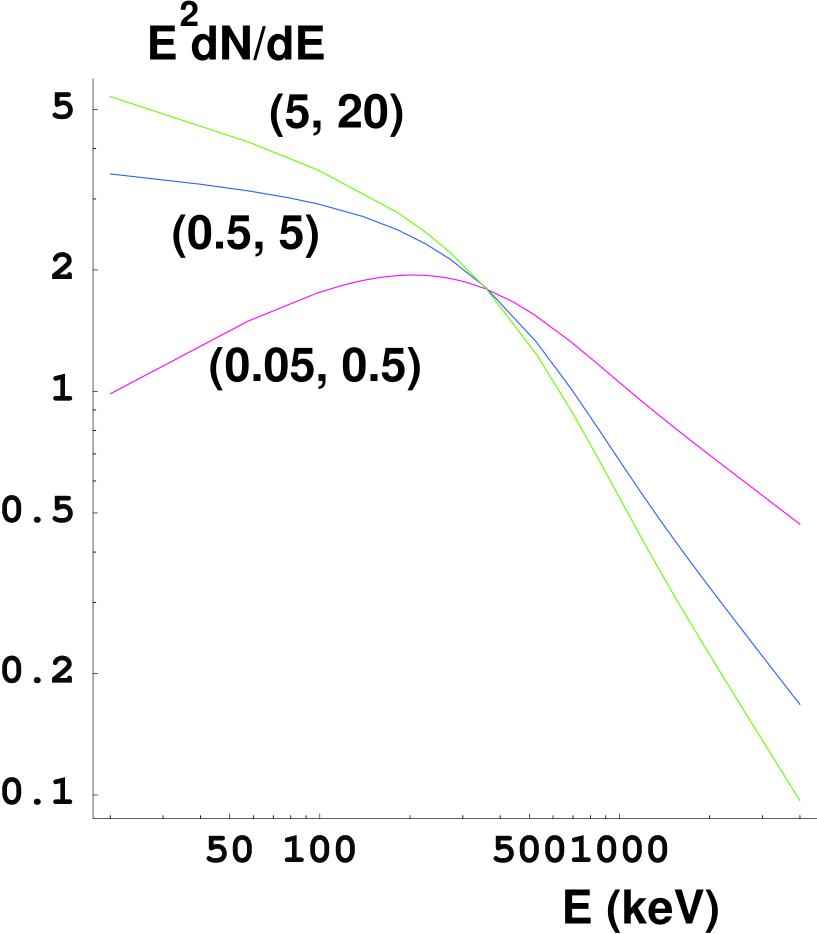
Figure 16: Spectral shapes $E^{2}\,dN/dE$, predicted by Eqs. (52, 53) at three time intervals within a pulse, shown in parenthesis in units of $t_{tr}$.

To illustrate the time–energy correlation embedded in Eq. (53) we present results for the times in units of the observer’s $t_{tr}$, with all parameters fixed at their “central” values: $t_{1}=t_{2}$, $m=n=2$ in Eq. (38), $b=1$ in Eq. (47), and $t_{c}=t_{tr}$, $\beta_{1}=1.6$, $\beta_{2}=2.1$ in Eq. (52). The parameter $T$ of Eqs. (38) and (53) is chosen such that the characteristic GRB energies are in the typical observed range, as in the prediction of Eq. (44). In Fig. (15) we show the pulse shapes (arbitrarily normalized for presentation) of a single GRB pulse in three energy intervals. The pulses are seen to rise faster and be narrower the higher the energy interval, as in GRB observations (e.g. Norris et al. 1996 ). In Fig. (16) we show the energy distributions $E^{2}\,dN/dE$ (arbitrarily normalized for presentation) at three time intervals within a pulse. The spectrum is seen to become softer as time evolves, as in GRB observations (e.g. Norris et al. 1996, Frontera et al. 2000).

There is another fact contributing to a non-trivial correlation between energy and time within a GRB pulse. The relation between the energy of a struck ambient photon, $E_{i}$ —or the temperature $T_{i}$ characterizing its initial distribution— and those of the resulting GRB photons, $E$ anf $T$, is that of Eqs. (21) and (44). As the CB reaches the more transparent outskirts of the wind, its ambient light distribution is bound to become increasingly radial, meaning that the average $1+\cos\theta_{i}$ in Eqs. (21) and (44) will depart from $\sim 1$ and tend to $0$ as $1/r^{2}$: the point-source long-distance limit. Since this transition depends on the integrated absorption by a wind with $\rho\propto 1/r^{2}\propto 1/t^{2}$, we characterize it by a simple time-dependence of the effective temperature in Eq. (47):

$$T\to T(t)\sim T\,\{1-exp[-(t_{T}/t)^{2}]\},$$ (54)

with $t_{T}={\cal{O}}(t^{w}_{tr})={\cal{O}}(t_{tr})$, see Eqs. (23) and (25). To investigate the incidence of a varying $T$ by itself (i.e. separately from that of an evolving $\tilde{p}$) we study the distribution:

$${dN\over dt\,dE}\propto{dN\over dt}\times{dN[T(t)]\over dE}\;,$$ (55)

with $dN/dt$ as in Eq. (38) and $dN/dE$ as in Eq. (47).

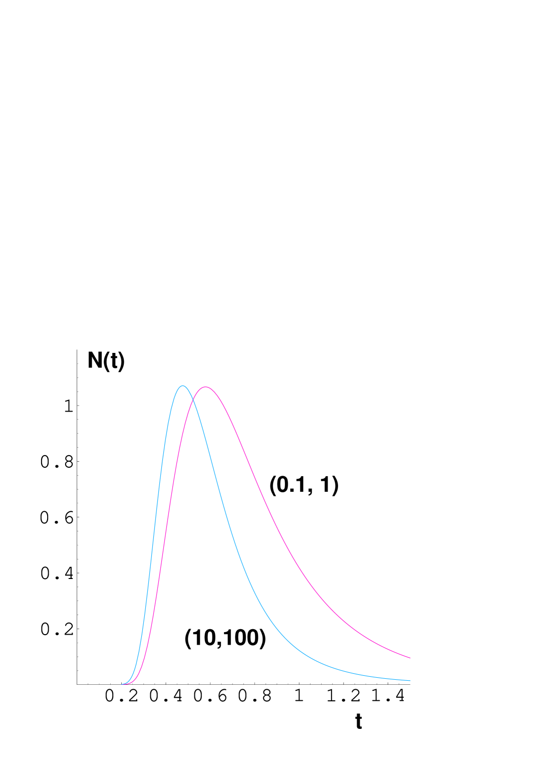
Figure 17: Pulse shapes $dN/dt$ (arbitrarily normalized for presentation) at two energy intervals, given in parenthesis in units of $T$ and corresponding to Eqs. (54, 55). The time is in units of $t_{tr}$.

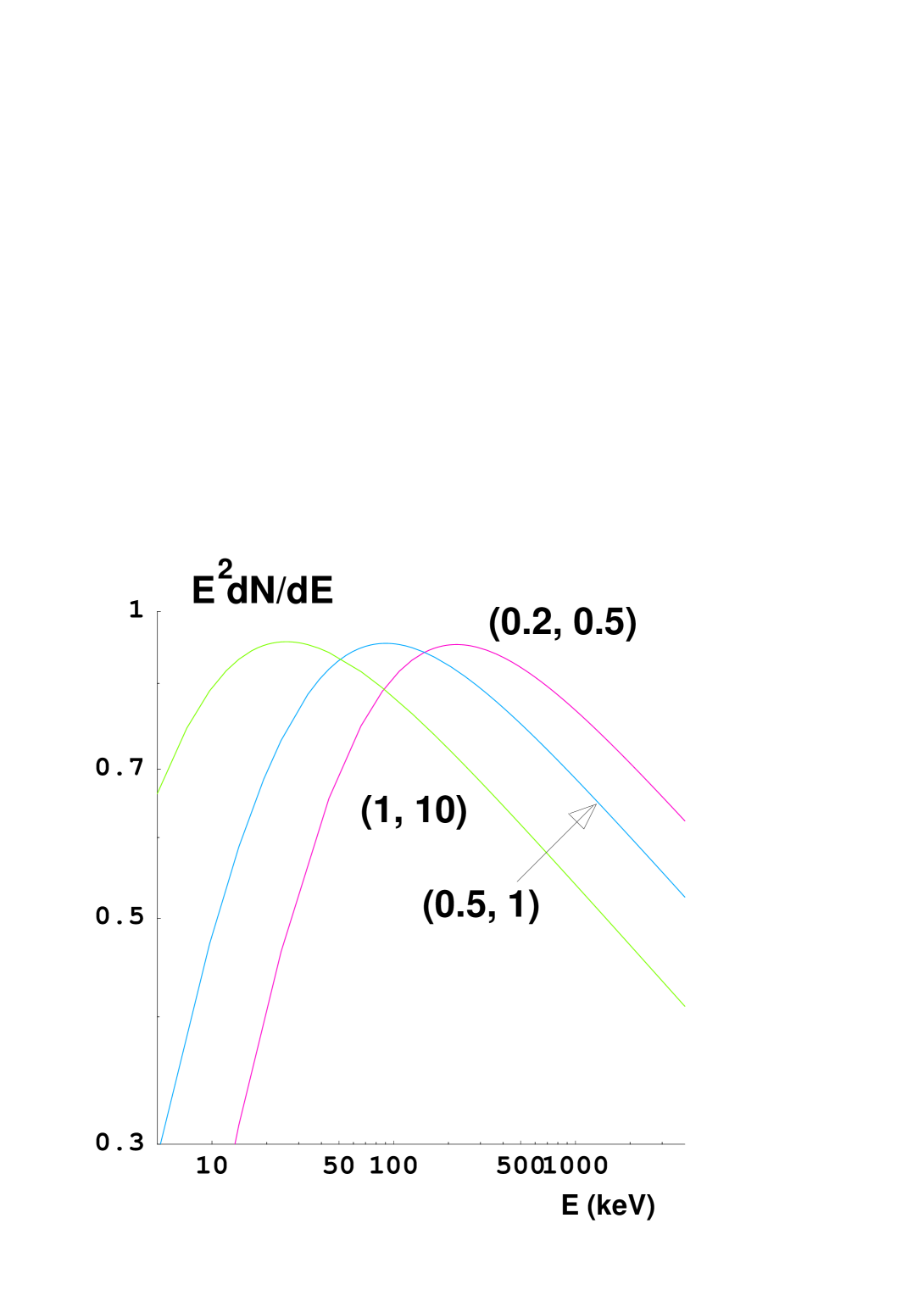
Figure 18: Energy distribution $E^{2}\,dN/dE$, at various times in a pulse, given in parenthesis in units of $t_{tr}$, and corresponding to Eqs. (54, 55).

To illustrate the time-energy correlation embedded in Eq. (54) and (55) we set all parameters to their reference values: $t_{T}=t_{tr}$ in Eq. (54), $t_{1}=t_{2}=t_{tr}$ in Eq. (38), $\alpha=1$, $\beta=2.1$, $b=1$ in Eq. (47). In Fig. (17) we show the pulse shapes (arbitrarily normalized for presentation) of a single GRB pulse in two energy intervals. Once again, the narrower and faster-rising curve is that corresponding to the higher energy interval, so that a varying temperature enhances the effect of a varying $\beta$, as in Eq. (52) and Fig. (15). In Fig. (18) we plot $E^{2}\,dN/dE$ for a single pulse in three time intervals. Naturally, the spectral shape is invariant, but the spectrum gets softer as time elapses within a pulse, adding to the similar effect induced by a time-dependent $\beta$. This effect, equivalent to a reduction with time within a pulse of its fitted peak energy in a Band fit, is also observed (e.g. Norris et al. 1996, Frontera et al. 2000).

We shall not embark here in a thorough analysis of GRB $(E,t)$ correlations, embodied in the combination of Eqs. (52), (53), (54) and (55), but we offer two simplified examples of their predictions.

The effect described by Eqs. (52) and (53) changes the shape of GRB spectra with time, but does not affect their energy scale, as the effect described by Eqs. (54) and (55) does. The dominant $(E,t)$ correlation is thus the one of the latter effect, which implies that $E$ and $t$, in $dN/dE$ appear in the combination $E/T(t)$. Since the (exponential) rise of a typical pulse, Eq. (37), is much faster than its (power) decay, the width of a peak is dominated by its late behaviour at $t>t_{tr}$. At such times, $T\propto 1/t^{2}$ in Eq. (54), so that $dN/dE$ is, approximately, a function of the combination $E\,t^{2}$. Consequently the width of a GRB pulse in different energy bands is:

$$\Delta t\propto E^{-\kappa},\;\;\;\;\;\;\;\kappa\;\hbox{\hbox to0.0pt{${}^{<}$\hss}${}_{\sim}$}\;0.5,$$ (56)

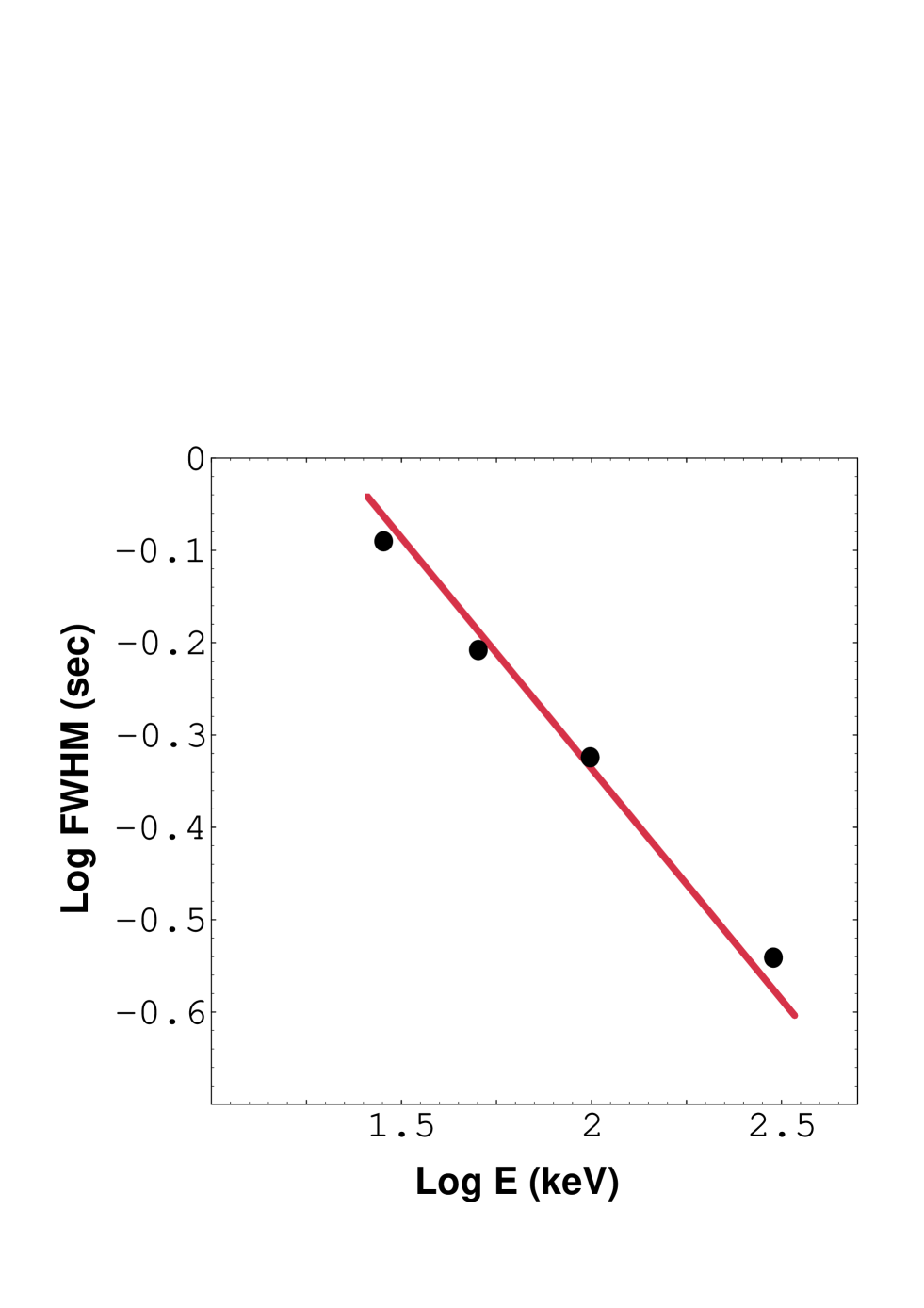
Figure 19: Average FWHM for the four BATSE energy channels, as reported by Fenimore et al. (1995) and Norris et al. (1996) compared with the prediction of Eq. (56). A more elaborate theoretical analysis would result in $\kappa\,\hbox{\hbox to0.0pt{${}^{<}$\hss}${}_{\sim}$}\,0.5$, a slightly less steep prediction.

where $\kappa=0.5$ is the limiting value for an exact dependence on $E\,t^{2}$. This result is in agreement with the observationally inferred relation $t_{{}_{\rm FWHM}}\propto E^{-0.43\pm 0.10}$ for the average FWHM of peaks as a function of the energies of the four BATSE channels (Fenimore et al. 1995, Norris et al. 1996), as shown in Fig. (19).

The width of successive pulses within a given multipulse GRB has also been studied by e.g. Ramirez-Ruiz & Fenimore (1999,2000), Ramirez-Ruiz, Fenimore & Wu (1999), Quilligan et al. (2002) and McBreen et al. (2002). The result is remarkably simple: the width of pulses of similar $E_{p}$ is independent of the time within the GRB’s duration at which they are located. In the CB model there is no reason for an “ageing” of the pulses: the ambient light that successive CBs scatter is time-independent, since the CBs do not “make a hole” in it.

The correlations between time and energy in a GRB pulse discussed in this section are dependent on the details of the CB model. Other correlations, which we proceed to review, are not “detail-dependent”, and have been discussed before (Dar & De Rújula 2000b; Plaga 2001).

13 More on correlations

13.1 “Relativistic” correlations between pulse properties

The CB model predicts very simple approximate correlations between pulse properties that depend only on special relativity (the various relations between times and energies reviewed in section 4.1 and the relativistic light-beaming effects discussed in section 4.2) and on general relativity (in the sense of involving the ubiquitous factor $1+z$ of an expanding Universe). Naturally, the correlations should be better satisfied if one can correct for the latter effect, as one can for the GRBs with known redshift, 32 at the time of writing.

If core collapse SNe and their environments were all identical, and if their ejected CBs were also universal in number, mass, Lorentz factor and velocity of expansion, all differences between GRBs would depend only on the observer’s position, determined by $z$ and the angle of observation, $\theta$. For a distribution of Lorentz factors that, as observed, is very narrowly peaked around $\gamma\simeq 10^{3}$, the $\theta$-dependence is in practice the dependence on $\delta$, the Doppler factor. This dependence is strong in various observables, e.g. cubic in the fluences of Eqs. (10), (12). Therefore, the correlations between these observables and others that are only linear or antilinear in $\delta$ —such as the energies in Eq. (4) and the times in Eq. (6)— are “strong correlations” and they might overwhelm much of the case-by-case variability induced by the distributions of the other parameters.

Let $\Delta t\propto 1/\delta$ be any measure of time, such as the width of a pulse, its rise time, or the “lag time” (the difference between the peak times of a given pulse in two different energy intervals). A measure of energy, such as the peak-energy $E_{p}$ in Band’s spectrum, is $\propto\delta$. The photon-number fluence is $f\propto\delta^{2}$, as in Eq. (9). The peak photon intensity $f_{p}$ (number of photons per unit time), the energy fluence, $F$ in Eq. (10), and the “isotropic” energy of a pulse, ${\cal{E}}^{iso}$ in Eq. (14), are all proportional to $\delta^{3}$. Finally, the peak luminosity $L_{p}$ (energy fluence per unit time) is proportional to $\delta^{4}$. All this implies, among others, the following correlations (Dar & De Rújula 2000b):

$$E_{p}\propto[\Delta t]^{-1}\,,$$ (57)

$$E_{p}\propto[f_{p}]^{1/3}\,;~{}~{}~{}~{}\Delta t\propto[f_{p}]^{-1/3}\,,$$ (58)

$$E_{p}\propto F^{1/3}\,;~{}~{}~{}~{}~{}\Delta t\propto[F]^{-1/3}\,,$$ (59)

$$E_{p}\propto[{\cal{E}}^{iso}]^{1/3}\,;~{}~{}~{}~{}\Delta t\propto[{\cal{E}}^{iso}]^{-1/3}\,,$$ (60)

$$E_{p}\propto[L_{p}]^{1/4}\,;~{}~{}~{}~{}\Delta t\propto[L_{p}]^{-1/4}\,.$$ (61)

The correlation of Eq. (57) is independent of redshift, all others should be better satisfied for pulses of GRBs with known redshift, after correction for the $z$-dependence.

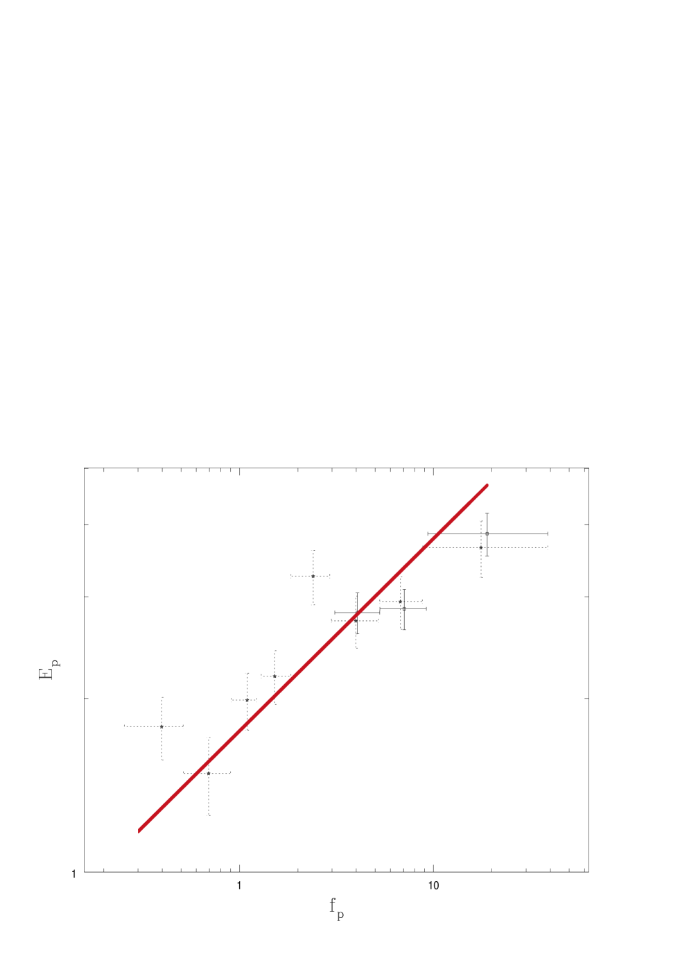
Figure 20: Average peak energy $E_{p}$, versus peak photon intensity $f_{p}$ in bins containing 20 GRBs of similar peak intensity (Lloyd et al. 2000). The line is the prediction of Eq. (58).

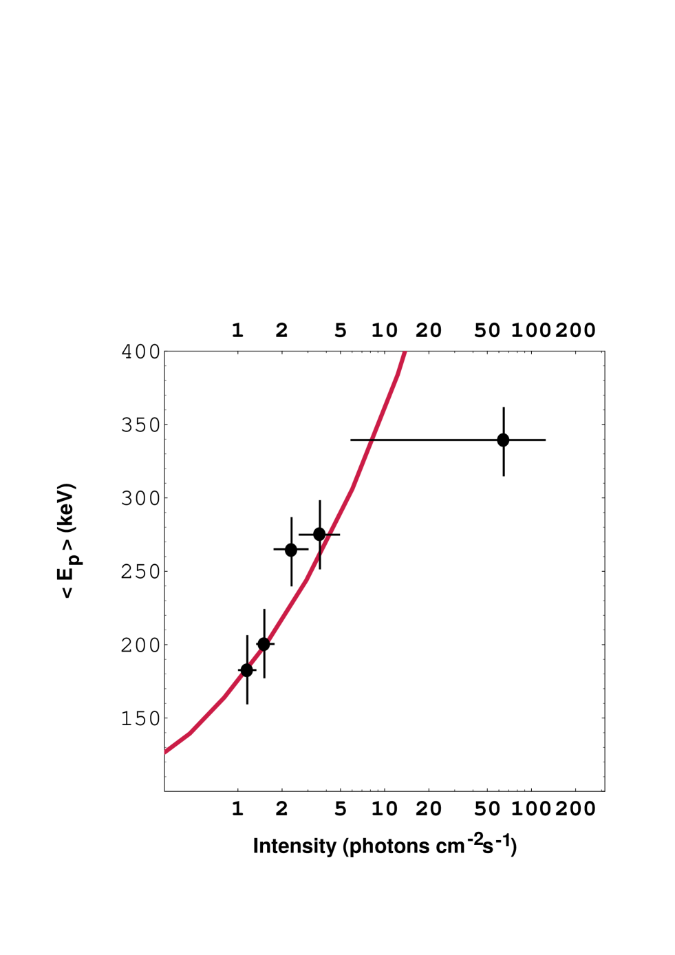
Figure 22: Averaged peak energy, $E_{p}$, versus peak photon intensity, $f_{p}$, from an analysis by Mallozzi et al. (1995). The line is the prediction of Eq. (58).

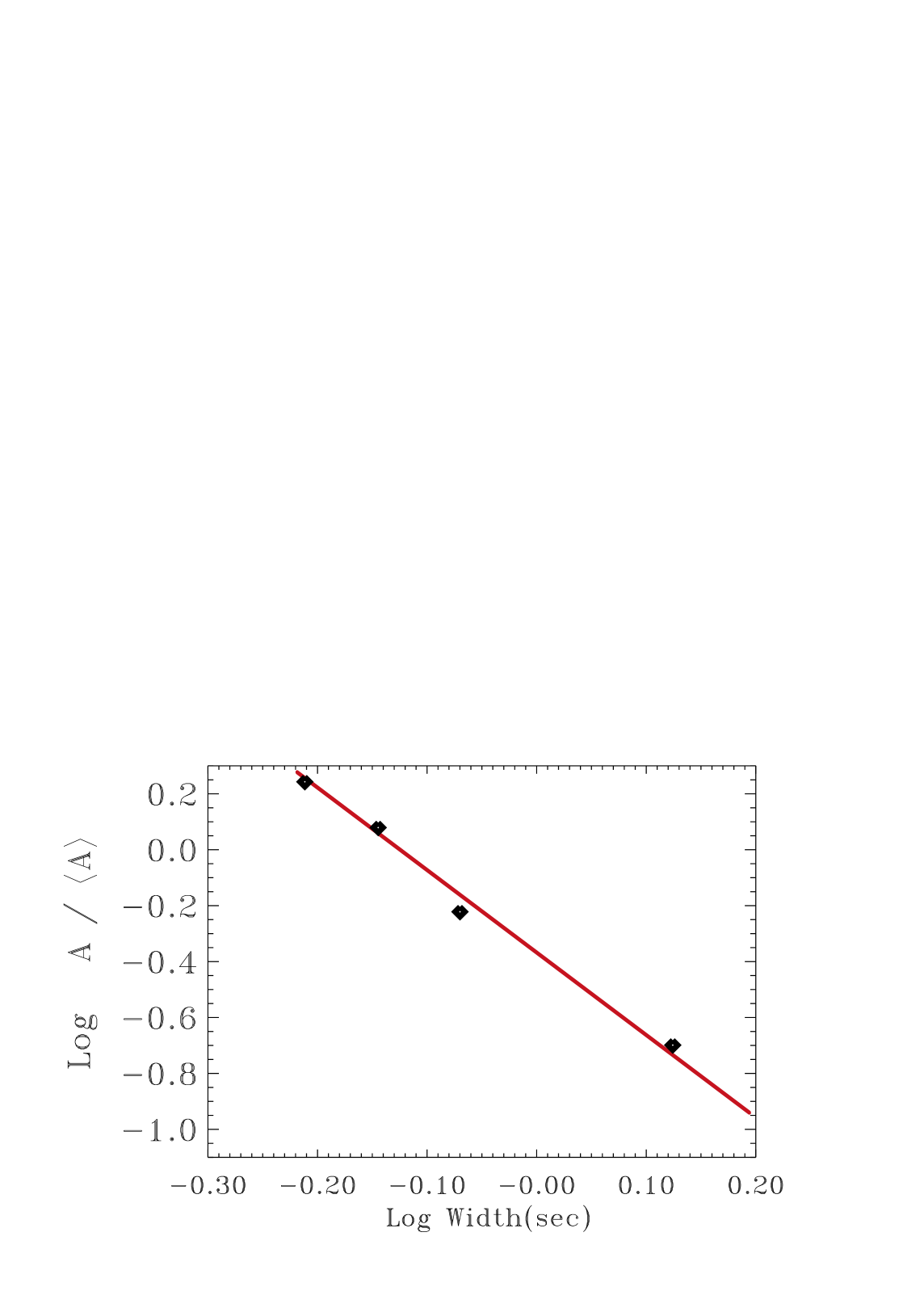
Figure 23: The ratio $A/{\langle A\rangle}\equiv f_{p}/{\langle f_{p}\rangle}$ versus the FWHM of GRB pulses, from Ramirez-Ruiz & Fenimore (2000). The line is the prediction of Eq. (58).

In Figs. (20) and (21) we show two examples of the above correlations: the average peak energy, $E_{p}$, versus peak photon intensity, $f_{p}$, and versus total fluence, $F_{tot}$, in bins containing 20 GRBs of similar peak intensity (Lloyd et al. 2000). The respective lines are the prediction of Eqs. (58) and (59). Another version of the $(E_{p},f_{p})$ correlation is that in Fig. (22), based on a data analysis by Mallozzi et al. (1995), where the line is again the prediction of Eq. (58). In Fig. (23) we show the prediction of Eq. (58) for the normalized ratio $f_{p}/{\langle f_{p}\rangle}$ of peak pulse fluences versus the pulse’s FWHM. The data analysis is from Ramirez-Ruiz & Fenimore (2000), who state: If we were to use the average point of all the normalized amplitudes in each selected range, the result is a power law: $f_{p}/{\langle f_{p}\rangle}\sim[{\rm FWHM}]^{-3.0}$. This is precisely the prediction.

A correlation that —to our knowledge— has not been investigated, is the following. The time delays between the pulses of a GRB are simply stretched by a factor $1+z$ relative to the emission times of the corresponding CBs at the location of the parent SN. The same is the case for the total duration of a GRB. On the other hand, the GRB energies and the time intervals within pulses, relative to their values in a CB’s rest system, are related as in Eqs. (4) and (6), which invlove the combination $\delta/(1+z)$. The consequent relations in Eqs. (56) and (57) are $z$-independent, while all of the other relations in Eqs. (58) to (61) have the explicit $\delta$ and $z$ dependences that can be read from Eqs. (9) to (15). All this opens a host of obvious combinatorial possibilities from which one could extract, in a statistical sense, GRB distributions in $z$ and $\delta$, which are explicitly testable for GRBs of known redshift. To give an example, the time intervals, $t_{int}$, between pulses increase with $z$ as $1+z$, while the widths of the pulses, $t_{FWHM}$, increase as $(1+z)/\delta$, with their “power” ($E_{p}\,\Delta t$) remaining constant. The ratio $t_{int}/t_{FWHM}\propto\delta$ is independent of $z$. Since at higher $z$ GRBs with higher $\delta$ (narrower pulses) are favoured by selection effects, this may in part explain the “Cepheid-like” correlation between variability and redshift advocated by Fenimore and Ramirez-Ruiz (2000) and by Reichart et al. (2001).

13.2 Correlations between global GRB properties

The correlations in Eqs. (57) to (61) apply to individual pulses and to pulse averages over a GRB. When applied to global GRB properties, some of these correlations are expected to have larger scatter than they have for individual or averaged pulses. An example is the correlation of any quantity with the total duration $W$ of a GRB, often defined as $t_{50}$ or $t_{90}$ for the per cent of total energy measured in a given time interval $t_{i}$. These correlations mix the pulse durations with the durations of the inter-pulse intervals which have, as discussed in the previous subsection, a different $\delta$ dependence. In Fig. (24) we show the trend of the observed GRB durations ($t_{90}$) versus the total energy fluence in the 7-400 keV band of 35 GRBs that were measured by HETE II (Barraud et al. 2003). The theoretical continuous line is the average trend expected in CB model for the width of the individual pulses. The theoretical dashed line is the expectation for the time intervals between pulses.

For GRBs with several pulses ($N_{p}\gg 1$), $W$ is approximately proportional to $N_{p}$, since the mean time interval between pulses is independent on the GRB’s duration (e.g. McBreen et al. 2002) and $N_{p}-1\approx N_{p}$. One may thus use this proportionality to obtain approximate correlations between global GRB properties (indicated by a GRB subindex), such as ${\cal{E}}^{iso}_{{}_{GRB}}\propto W\,{\langle E_{p}\rangle}^{3}$ and $F_{{}_{GRB}}\propto W\,{\langle E_{p}\rangle}^{3}$, with $\langle E_{p}\rangle$ the average of the peak energies of the pulses in a given GRB. Such relations are also well satisfied by the observations.

The time variability of a GRB is a “global” measure of an inverse time, $V\propto L_{p}^{-1/4}$, according to Eq. (61). This variability–luminosity relation is shown in Fig. (25), for GRBs of known redshift (Reichart et al. 2001). An example of the variability–peak energy correlation in Eq. (61) is given in Fig. (26), in which the data analysis is from Ramirez-Ruiz & Lloyd-Ronning (2002).

14 A detailed example: GRB 980425

This GRB and its associated supernova, SN1998bw —both traditionally considered entirely exceptional in the FB models— are the battle-horses of the CB model. Neither of them is —in the CB model— a special class onto itself:

• In Dar & De Rújula (2000a) we argued that the only peculiarity of GRB 980425 was its nearness ($z=0.0085$), which allowed for its detection at an angle, $\theta\sim 8$ mrad, unusually large with respect to that of all other GRBs of known redshift, for which $\theta\sim 1$ mrad. These facts conspired to produce a “normal” GRB fluence —given the strong $\delta$-dependence of Eq. (10)— and resulted in an optical AG dominated by the SN.

• In Dado et al. (2002a) we demonstrated that the X-ray AG of this GRB was also “normal”: it has precisely the light curve (in shape and normalization) expected in the CB model if the X rays are produced by the CBs and not, as the observers assume (Pian et al. 2000), by the associated SN. Moreover, subsequent X-ray data from XXM Newton and Chandra (Pian et al. 2003) agree exactly with the prediction in Dado et al. 2002a; 2003a).

• In Dado et al. (2003a) we demonstrated that the radio AG of this GRB was also “normal”: it has precisely the normalization, spectrum and fixed-frequency light curves expected in the CB model if the radio emission is produced by the CBs and not, as the observers assume (e.g. Kulkarni et al. 1998), by SN1998bw.

• Deprived of the X-ray and radio emissions that it did not emit, SN1998bw loses almost all of its alleged exception. Its only peculiarity was that it was viewed very near its axis, in comparison with ordinary SNe. This is no doubt the reason why exceptionally high velocities ($v\sim 23,000\pm 3,000\,{\rm km\,s^{-1}}$) for its expanding shell were deduced from observations of its line emissions (Patat et al. 2001). Indeed, the exiting jets of CBs are surely accompanied by a fast outward motion of the SN shell in its “polar caps”. Viewed almost on-axis, such motions should result in highly Doppler-boosted line emissions.

• Since GRB 980425 was an ordinary GRB it makes sense —in the CB model— to use SN1998bw as a potential standard candle, or standard-torch, associated with other GRBs (Dar 1999a,b). This naive hypothesis has met an incredible success. In all GRB AGs for which such a SN contribution could in practice be discerned, the contribution was discernible, with various degrees of significance (Dado et al. 2002a). In four cases Dado et al. 2002a,b; 2003e,f) we predicted the presence of a SN1998bw-like contribution from AG data taken before the SN was observable. The last and quite impressive case is that of GRB 030329 and SN2003dh (Dado et al 2003f; Stanek et al. 2003).

In this section we complete our argument regarding the “normality” of GRB 980425 by studying in more detail the $\gamma$-rays of its burst.

The total observed fluence of this GRB was (Kippen et al. 1998; Frontera et al. 2000):

$${dF\over d\Omega}={1\over 2\pi}\,{dF\over d\cos\theta}\simeq 0.44\times 10^{-5}\;\rm erg\;cm^{-2},$$ (62)

comparable to that of other GRBs of known redshift, but corresponding to a spherical-equivalent energy $8.1\times 10^{47}$ erg, some five orders of magnitude smaller than average. The energy-integrated spectrum was analysed in the Band model by Yamazaki, Yonetoku & Nakamura (2003), with the result that $\alpha=1\pm 0.3$, $\beta=2.1\pm 0.1$, both perfectly compatible with the central expectations of Eq. (47). The peak energy was found to be:

$$E_{p}=54.6\pm 20.9\;\rm keV,$$ (63)

anomalously small by average standards. The energy spectrum in various energy bands is shown in Fig. (27), from Frontera et al. 2000. The shape of the single pulse (or single dominant CB) of this GRB, in the 50–300 keV energy band (Kippen 1998), is shown in Fig. (28).

The relative smallness of the fluence of this GRB can be trivially understood (Dar & De Rújula 2000a). For a rough estimate, take the single CB’s rest-system energy output to be that of Eq. (34), with all parameters fixed at their reference values. We may then use $dF/d\Omega$ as in Eq. (10) and the known distance to the progenitor (39 Mpc for $H_{0}=65$ km s^-1 Mpc^-1) to obtain the value of $\delta$ that would reproduce the observation in Eq. (62): $\delta\sim 20$.

With the above value of $\delta$ and all other parameters fixed at their reference values, we may proceed to investigate whether or not the $\gamma$-ray pulse of GRB 980425 was in any sense exceptional. From Eq. (21) we obtain a peak energy of 20 keV, fairly close to the 1$\sigma$ lower limit of Eq. (63). For the full width at half-maximum of the pulse’s peak we obtain 11.6 s, by use of Eq. (23), in agreement with the observation reported in Fig. (28).

In Dado et al. (2003a) we obtained the parameters $\theta$ and $\gamma$ for this GRB from the observations of its radio AG: $\theta=7.83$ mrad, $\gamma=495$, corresponding to $\delta=62$. These parameters are not as well determined as for other GRBs, since we have no information on the optical AG, which, given the large value of $\theta$, was overwhelmed by the light of SN1998bw. Moreover, the X-ray data for this GRB are quite poor, and the radio AG, which is well measured is (at the large $\theta$-value of this GRB) most sensitive to details such as the CB’s geometry (the radio emission originates in the CB’s surface, as opposed to the higher-frequency AG emissions, to which the CB is transparent). We therefore do not consider the “large” discrepancy between $\delta=62$ and $\delta=20$ to be a problem, particularly since the $\gamma$-ray properties of this GRB could be easily described with either $\delta$, should we be willing to moderately depart from the use of the reference values for the rest of the parameters in Eqs. (21), (23). It is clear that —in the CB model— GRB 980425 was not exceptional, and we may proceed to study its spectrum and light-curve in more detail.

To describe the spectrum of GRB 980425 in various time brackets, we use Eq. (47), with $\alpha=b=1$, their reference values and $T=E_{p}$, given in Eq. (63). The quantity $\beta$ in Eqs. (47) and (52) is allowed to evolve from a value $\beta_{1}=1.6$ to $\beta_{2}=2.3$ —the observed $\beta$ peak value, as in Fig. (13)— according to Eq. (52), with $t_{c}=t_{tr}^{w}/2$ (this is the only parameter we choose not to have its precise reference value). We also allow for the effect of a varying $T(t)$, as in Eq. (54), with $t_{T}=t_{tr}$, its reference value. For each time bracket we present results for the corresponding average time, since the brackets are narrow and a time-integration insignificantly affects the results. The result of this exercise is shown in Fig. (27) and is quite satisfactory, considering that we are “describing”, rather than fitting, the spectral evolution.

In Fig. (28) we repeat the above exercise, with the same parameter choices, to describe the very good data on the pulse-shape of GRB 980425 in the 50–300 keV bracket. This time the bracket is wide, and we have integrated $dN/dt\,dE$ in the quoted energy interval. The result, naturally, is sensitive to the width of the pulse, which we have taken to be the observed $\sim 25$ s full width at half-maximum of the pulse integrated over all observed energies (Frontera et al. 2000).

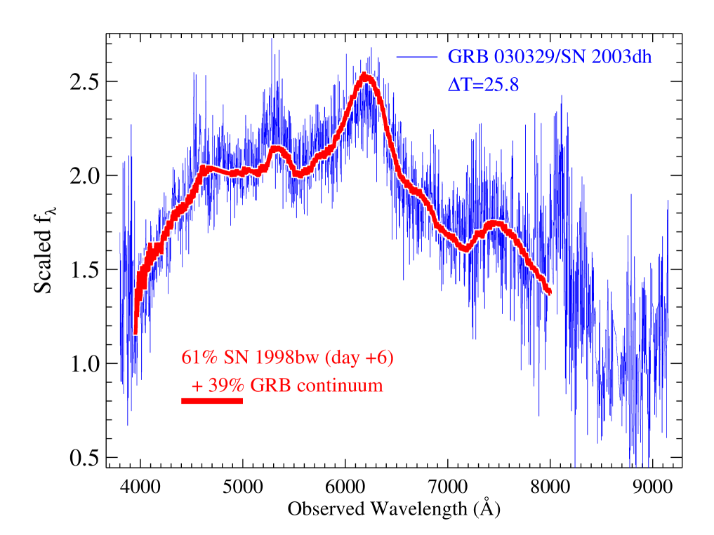
Figure 29: Comparison of the optical spectra of SN2003dh and SN1998bw (Matheson et al. 2003).

Our results prove that GRB 980425 was a perfectly normal GRB that just happened to occur nearby, and to be observed at a comparatively slant angle. This makes the use of its associated SN —as a putative standard candle, or standard torch, for other SNe associated with GRBs— a reasonable undertaking. The next best-measured GRB-associated SN is the next closest one: SN2003dh, associated with GRB 030329 (Stanek et al. 2003). SN2003dh and SN1998bw look like identical twins, as shown in the comparison of their spectra in Fig. (29), from Matheson et al. (2003).

15 The parameters of the cannonball model

More often than not, the description of astrophysical phenomena involves parameters that are chosen “just so” that the desired result is obtained. As we discuss in Section 19 and Appendices II and III, the FB models of GRBs are no exception. The CB model is.

CBs decelerate in the interstellar medium by “collisionless” interactions with the ISM’s heavy constituents: protons and nuclei, which bounce off their enclosed magnetic field. The particles recoiling from a single such collision have energies extending up to $E_{max}=2\,\gamma^{2}\,M\,c^{2}$ (or even larger in the case of multiple collisions). The particles thus accelerated are the cosmic rays of the GRBs’ host galaxy. These $M$-dependent values of $E_{max}$ coincide with the “knees” in the cosmic-ray spectra for $\gamma\simeq 10^{3}$, and qualitatively explain their features (Dar & Plaga 1999). Thus the ab initio choice of the typical $\gamma$ (Dar & De Rújula 2000a).

The initial expansion velocity of a CB is naturally chosen to be of the order of the speed of sound in a relativistic plasma, i.e. $\beta_{s}\sim 1$. The photon-number density of the ambient light and the winds’ density we use here originate in observations. The observer’s angle $\theta$ is, like the redshift $z$, not a property of the CBs themselves.

The large peculiar velocities of neutron stars, $\langle v\rangle\!\sim\!450$ km s^-1, are attributed, in the CB model, to an imbalance in the momentum of the two opposite jets of CBs that accompany their birth (Dar & Plaga 1999). Neither that imbalance (perhaps 50%) nor the average number of significant CBs per GRB (perhaps 10) can be easily ascertained. The choices in parenthesis and an initial $\gamma=10^{3}$, for stars of mass 1.4 $M_{\odot}$, yield an a priori rough estimate, $N_{{}_{B}}=5\times 10^{50}$, for the CB baryon number. In the study of AGs, a deceleration parameter $x_{\infty}$ is introduced. It governs the slow-down of CBs by collisions with the ISM. Its value is fixed by $N_{{}_{B}}$, the ISM density, and the calculable fixed asymptotic value of the CB’s radius, reached within a few minutes of observer’s time. The values of $x_{\infty}$ that the AG fits return are in the anticipated range (Dado et al. 2002a). In Dado et al. (2003a) we found that our ab initio parameter choices resulted in a one order of magnitude overestimate of the AGs’ absolute luminosity. Whence our slight reduction of the originally adopted $N_{{}_{B}}$, by a factor of $\sim 6$.

In the discussion of the wide-band spectrum of a GRB AG, only one extra independent parameter must be introduced, a free-free absorption frequency $\nu_{a}$, describing the attenuation of radio waves at a CB’s surface. This is the only parameter for which we do not have a solid a-priori estimate.

In this paper we have introduced a series of parameters pertinent to the description of a GRB itself: $t_{1}$ and $t_{2}$ in Eq. (38), $\alpha$, $\beta$ and $b$ in Eq. (47), $\beta_{1}$, $\beta_{2}$ and $t_{c}$ in Eq. (52). These are quite a few parameters, but their central predicted values coincide with those deduced from observations. Here the only exception of a parameter for which we have not attempted to derive an a-priori value is $b$ in Eq. (47), which sets the relative contributions of accelerated and unaccelerated CB electrons to the GRB energy spectrum.

The conclusion of this section is that it is fair to say that the overwhelming majority of the parameters of the CB model either have theoretically predicted central values in agreement with observations or —since CBs play a role in areas of astrophysics other than GRBs— are not specifically fine-tuned to the GRB observations.

16 Limitations of our current analysis

16.1 The timing of the CB emission

Two time scales characterize the infall of material onto the newly formed compact object resulting from the collapse of the core of a star. One is the infall time of matter in the immediate vicinity of the pre-collapsed core, of the order of tens of seconds. The second, of the order of hours, is the fall-time of material from the outer layers of the pre-collapsed star. There is no a-priori way of knowing whether the accreting disk or torus, whose further successive episodes of violent accretion generate the CBs, is formed on the first or the second time scale. Current models of SN explosions do not explode SNe, unless some ad-hoc physics is added to them: the position where their “shocks stall” may not be a serious indication of the location of matter that may “fall-back”. The only indication of a “double bang” in a SN (De Rújula 1987) was provided by SN1987A, which generated two neutrino bursts, one irrefutable in its statistical significance (Bionta et al. 1987; Hirata et al. 1987) the other much less so (Aglietta et al. 1987). These bursts, both lasting a few seconds, were separated by some 5 h.

In our original model, we assumed that the CBs were emitted a few hours after core-collapse (Dar & De Rújula 2000a). We have implicitly made here the same assumption, for it also takes hours for the information that the core has collapsed to reach the surface of the parent star, the moment at which the star’s luminosity rises sharply to ionize and illuminate its prior wind. But we do not know whether or not processes occurring prior to the collapse, such as the violent wind-illuminating episode shown in Fig. (1) may be the ones responsible for generating the ambient echo light. In this latter case there would be only one time-scale associated with GRBs: the shorter one. This, if the second neutrino bang of SN1987A is simply ignored, is an attractive possibility.

The only methods to tell apart the one-time and two-time scenarios with the help of GRB observations are to measure the timing of a GRB relative to the prompt flash of its associated SN (difficult, because the signal is superimposed on the AG “background”), or relative to the thermal neutrino flash (a dream). The launching of CBs from the SN’s central region ought to be accompanied by the emission of gravitational waves, which are much more isotropic than the GRB (Segalis and Ori 2001). An observation of these waves in coincidence with a GRB (most unlikely) or with a SN explosion (not out of the question) would also help. Finally, it is conceivable that a convincing double bang be observed in the form of two separate thermal neutrino bursts from a SN explosion in the Galaxy or the Magellanic Clouds.

16.2 The GRB energy emitted by a single CB

In Section 8, we compared the prediction for the total energy, ${\cal{E}}^{\prime}_{CB}$, emitted by a single CB in its rest system —in the form of photons that an observer sees as $\gamma$-rays— with the range of values (0.6 to 2.1 times $10^{44}$ erg) that we had previously extracted from analyses of GRB AGs (e.g. Dado et al. 2002a). The question is: Does this “observed” range correspond to the emission by a single CB?

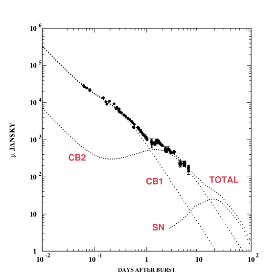
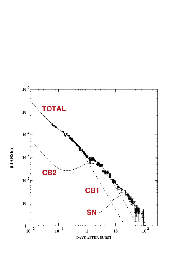
Figure 31: Upper panel: The R-band AG of GRB 030329, used along with other optical data to predict, in the CB model, the presence of a SN akin to SN1998bw (Dado et al. 2003f). Lower panel: The subsequent data (the $\star$ symbols) are added.

Two cases in which the answer is affirmative are: GRB 030329 (Dado et al. 2003f), which we discuss in further detail in Appendix I, and GRB 021004 (Dado et al. 2003c). These cases have various common properties: the GRB’s $\gamma$-ray light curve has a very clear two-peak (two-CB) structure, as can be seen in Fig. (30); the AG fluence evolution has two humps which correspond, in the CB model, to the individual contributions of the two CBs, as in Fig. (31); and the AG of both GRBs was “caught” very early: good measurements of it were taken before $t\sim 1$ day. This allowed us to perform analyses in which the extracted ${\cal{E}}^{\prime}_{CB}$ indeed corresponds to each single CB.

Several other cases we have studied (such as GRB 980425, discussed in detail here and in Dado et al. 2003a) the GRB light curve has a single or a single-dominant CB. For these cases the answer is also affirmative. But there are cases, such as that of the fluence record-breaking GRB 980123, in which the GRB light curve has several clear pulses. In most of these cases, however, the AG was caught at a relatively late time, so that it is quite possible that it was dominated (as the relatively late time AG of GRB 021004 or GRB 030329 is) by a single CB. In that case, the value we extracted for ${\cal{E}}^{\prime}_{CB}$ would also correspond to just one CB.

Finally, there may be a small fraction of cases in which the AG, analysed by us as if due to a single CB, received comparable contributions from various CBs, with similar Lorentz factors and emission angles. For those cases, our extracted ${\cal{E}}^{\prime}_{CB}$ corresponds to a sum of CBs, and the “real” single-CB number would be smaller by a factor of a few. This does not detract much from the striking coincidence between the range of “observed” values of ${\cal{E}}^{\prime}_{CB}$ and the prediction of Eq. (34).

16.3 The coalescence of CBs

Two CBs emitted roughly in the same direction, at times differing by $\Delta t$ in the SN rest frame, may coalesce on their way to the observer, if the Lorentz factor, $\gamma_{2}$, of the second one is larger than that of the first, $\gamma_{1}$. Is this a complication that needs to be addressed in detail? The short answer is: No. Thus, we shall discuss the issue with all parameters set at their reference values, but for one of the Lorentz factors.

The typical separation of pulses in a long-duration GRB is of ${\cal{O}}(1\,\rm s)$ which, at a typical $z=1$, corresponds to $\Delta t=2$ s in the local SN rest frame. At the CB-transparency time at which the bulk of its GRB pulse is emitted, a CB has moved to a distance $r_{tr}\sim 7\times 10^{15}$ cm from the SN, see Eq. (24). Consider first two CBs emitted with the same $\gamma$ and in the same direction $\theta$ at times 0 and $\Delta t$. Their centres would travel at a constant distance $d=c\,\Delta t=6\times 10^{10}$ cm, but could their expansion make them touch? The CBs’ longitudinal expansion rate in the SN frame is a factor $\gamma$ smaller than in the CBs’ rest frame, so that their longitudinal dimension at transparency time is $l=R_{tr}/\gamma\sim 4\times 10^{9}$ cm, where we have used Eq. (22). Since $l\ll d$, the answer is negative, unless $\Delta t$ happens to be much smaller, but in that case the pulses of the two CBs would be superimposed anyway. This takes us to the next case in point: $\gamma_{2}>\gamma_{1}$.

The time it takes the centres of two CBs emitted in the same direction, at an interval $\Delta t$, to have their centres touch is:

$$t_{merge}={\Delta t\over\beta(\gamma_{1})-\beta(\gamma_{2})}\simeq 2\,\Delta t\;{\gamma_{1}^{2}\;\gamma_{2}^{2}\over\gamma_{2}^{2}-\gamma_{1}^{2}}.$$ (64)

For $\gamma_{2}=2\,\gamma_{1}=10^{3}$, the corresponding merger distance is $c\,t_{merge}=4\,\times 10^{16}$ cm, about one order of magnitude larger than $r_{tr}$ in Eq. (24), the distance at which the GRB pulse is emitted, so that, typically, a CB–CB coalescence would not be observed in the GRB phase, but in the very early AG phase.

The ratio $c\,t_{merge}/r_{tr}$ is sufficiently close to unity that we may ask: What happens in the unlikely case that two CBs do merge? The electron constituency of the merged object will be boosted to a somewhat higher energy, by the shockless acceleration process we have advocated (at the relatively small relative Lorentz factor). The merger takes a time $\sim 2\,R_{tr}/c$ in the merged CB’s rest frame, and a cosmological observer sees it shortened by a factor $(1+z)/\delta$ to $\sim 1/2$ s, for typical parameters. Since at the time of merging the two CBs are already transparent, or nearly so, their total ICS signal, proportional to the sum of their baryon numbers, as in Eq. (36), is not significantly affected, but the sudden modest hardening of the electron spectrum would give rise to a hardening of the spectrum during a pulse.

Finally, we may ask how close the angles, $\theta_{1}$ and $\theta_{2}$, of the emission of two CBs must be, in order for a merger at the GRB-emission (or CB-transparency) time to be at all possible. At the merger time, the CBs are at a distance $r_{tr}=\sqrt{3}\,\gamma\,R_{tr}/\beta_{s}$ away from the SN, and at a transverse distance $d_{t}=|\theta_{2}-\theta_{1}|\,r_{tr}$ from each other. For that distance to be smaller than $R_{tr}$ (so that they touch), it is required that $|\theta_{2}-\theta_{1}|<\beta_{s}/\sqrt{3}\,\gamma$. For $\beta_{s}$ close to its upper limit 1 that is fairly probable, so that our previous conclusions stay put.

If two or more CBs merge during the late GRB phase, the number of CBs that give rise to the AG may be reduced, relative to the number of significant pulses in the GRB. This would go in the direction symplifying the analysis of AGs and reducing the spread in the values of ${\cal{E}}^{\prime}_{CB}$ extracted from fits to the AGs, which is observed to be very small.

16.4 Other $\gamma$-ray emitting mechanisms

The shell of ejecta of a SN should not be spherically symmetric, for various reasons. The angular momentum of the parent star implies that its collapse should be faster close to the poles than to the equator. The exiting jet of CBs no doubt affects the shell around its polar caps. Assuming these effects not to be very important —that is, in the approximation of a spherically symmetric shell— we estimated in Dar & De Rújula (2000b) how the collisions of the CBs with the shell material would heat the CBs. We conjectured that a GRB pulse would be the radiation emitted by the heated CBs, visible after the CBs enter the transparent outskirts of the SN shell, and would diminish in temperature (and $\gamma$-ray energy) as the shell’s material thins down. We found that two models along this line (a “surface-” and a “volume-” heating model) were also very successful in predicting all the properties of a GRB pulse for CB parameters in the range we have rediscussed here. Why then do these quasi-thermal (QT) variants of the CB model not imply that there is an additive contribution to the ICS process discussed in this paper?

The simplest answer to this question is that such a contribution may indeed be there. The second simplest answer is that the assumption of spherical symmetry may be very wrong: the polar regions of the SN shell may be depleted in density, in which case the quasi-thermal GRB-generating process would be subdominant. We subscribe to the second possibility for the following reasons:

• The QT models predict a vanishing GRB polarization.

• In each QT model we had to make one rough approximation. In the simplest “surface model”, for instance, we assumed that all the heat hadronically deposited in a GRB within a photon’s interaction length from its surface was instantaneously re-emitted. The beauty of the ICS process that we have discussed here is that no such approximations have to be made: all the physics is simple, transparent and unquestionable.

17 Are short GRBs generated by Type Ia SNe?

We contend that, in the CB model, it is very natural to answer the question affirmatively (Dar & De Rújula 2003): the observed properties of short GRBs are understood in much the same way as those of the long-duration ones, which we discussed so far. The information we have about Type Ia SNe, however, is very meager relative to that on core-collapse SNe, which encompass all other spectroscopic types. Thus, our considerations stand on less firm grounds. Yet, as we shall see, the model explains why the AG of short-duration GRBs should be hard to detect. This means that observers should look in the GRB’s direction not only as fast as possible after the GRB time (in case an AG is discernible) but also about one month later, when it should be possible to discover the allegedly associated Type-Ia SN around its peak luminosity. Such a SN, if it is there, may not look identical to the standard-candle Type Ia SNe so useful in cosmology, for it would be viewed nearly on-axis.

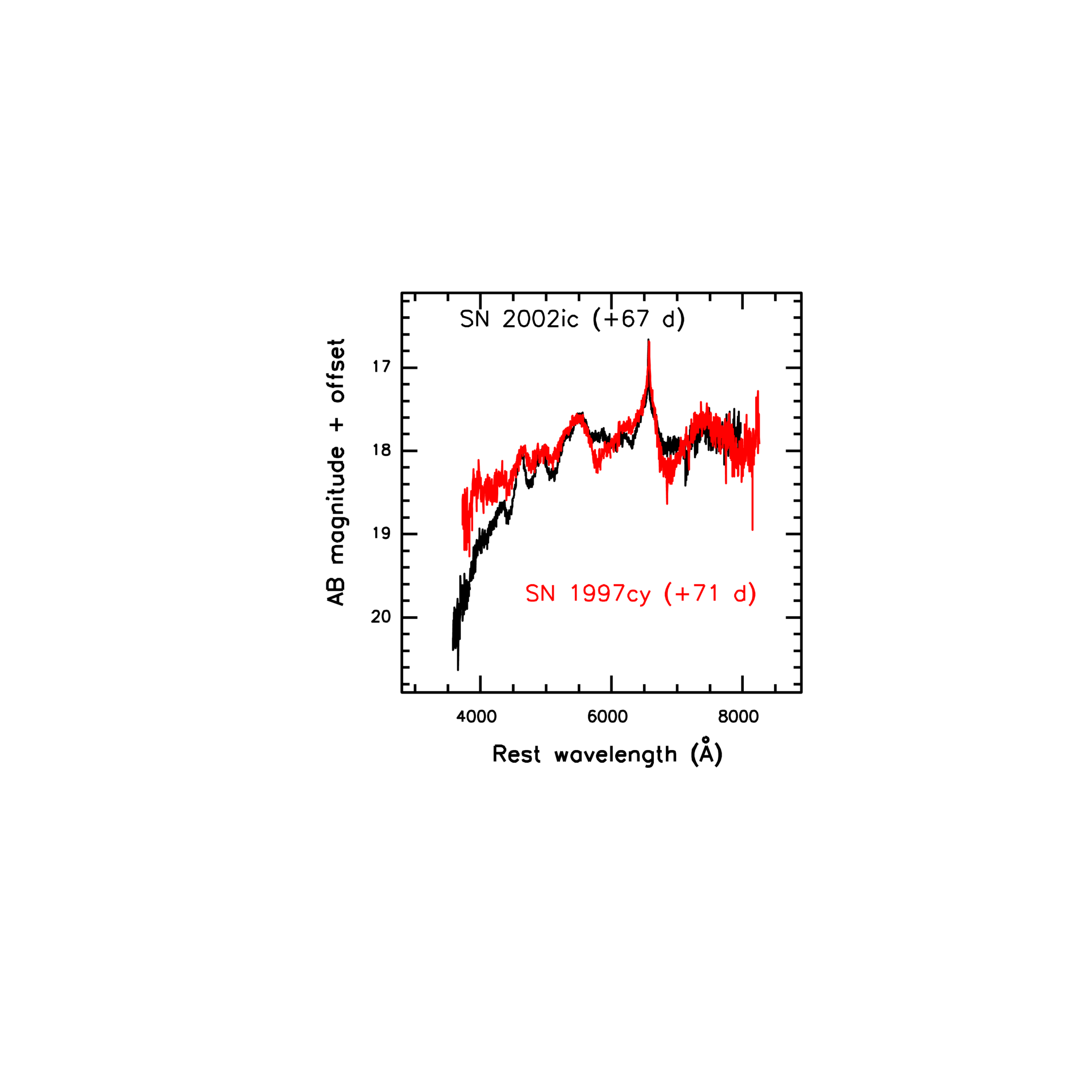
Figure 32: Comparison of the optical spectra of SN2002ic and SN1997cy (Hamuy et al. 2003).

Our suggested association of short-duration GRBs with Type Ia SNe (Dar & De Rújula 2003) appeared to be in conflict with the possible association (Germany et al. 2000) of the short-duration ($\sim 0.2$ s) GRB 970514 with SN1997cy at $z=0.07$, which is Type IIn, and not Type Ia. But this situation was recently reversed. Hamuy et al. (2003) observed that SN2002ic at almost the same redshift, $z=0.0666$, —whose Type is Ia— had a spectrum almost identical to that of SN1997cy. Moreover, unexpectedly, its spectrum also featured a narrow H$\alpha$ line of FWHM $<300$ km s^-1, on top of a broader line of FWHM $\sim 1800$ km s^-1, see Fig. (32). Hamuy et al. (2003) suggested that the identification of SN1997cy as Type IIn could have been wrong, and that most probably it was of Type Ia, like SN2002ic. They also concluded from the light-curve and the lines of SN2002ic that the explosion’s energy, like that of SN1997cy, was unusually high, $\sim 3\times 10^{52}$ erg. Since the thermonuclear explosion of a carbon–oxygen Chandrasekhar white dwarf is very unlikely to produce more than $2\times 10^{51}$ erg (Arnett 1996), we must conclude that Type Ia SNe are more axially than spherically symmetric and that SN1997cy and SN2002ci were observed close to their jet axis, like SN1998bw. There, the expansion velocity is naturally much higher than near the equator, leading to an overestimate of the explosion’s energy.

17.1 Type Ia SNe

Little is known for sure about the progenitors or the production mechanisms of Type Ia SNe. The prevailing theory is that accretion onto a $C/O$ White Dwarf (WD) from a companion star in a close binary system causes their collapse —accompanied by a thermonuclear explosion— when the accreting WD’s mass exceeds the Chandrasekhar limit (Whelan & Iben 1973). In the case of a WD–WD binary, the trigger may also be a merger, the end-result of a shrinking of the orbit due to gravitational-wave emission (Iben & Tutukov 1984; Webbink 1984).

In every one of the quoted scenarios, the specific angular momentum of the collapsing system is likely to be large. It is natural to expect that the collapsing object may have an axial symmetry leading to the bipolar ejection of jets of CBs, as in quasars, microquasars and the core-collapse SNe responsible —in the CB model— for long-duration GRBs. About $70\%\pm 10\%$ of all SN explosions in the local Universe are of the core-collapse types, the rest being Type Ia SNe (Tamman, Loeffler & Schroder 1994; van den Bergh & McClure 1994). Intriguingly, $\sim 75\%$ of all GRBs are long and the rest are short. The coincidence may not be accidental.

17.2 The environment of Type Ia SNe

The narrow lines and light curves of SN1997cy and SN2002ic have been interpreted as evidence for a circumstellar wind ejected from the WD’s companion, or from prior successive thermonuclear explosions on the WD’s surface (Chevalier 2003). In all other Type Ia SNe there is no evidence for circumstellar wind but the mass-loss rate is believed to be one to two orders of magnitude smaller than that from the progenitors of core-collapse SNe. The theoretical models of Type Ia SNe suggest that their wind intensifies as the collapse approaches, generating a surface density $\rho(r)\,r^{2}\sim 10^{15}$ g cm^-1 in their near environment (Chevalier 2003), an order of magnitude smaller than that for core-collapse SNe, Eq. (1). Such a wind becomes optically thin to Compton scattering at $r_{tn}^{w}\simeq\sigma_{{}_{T}}\,\rho(r)\,r^{2}/m_{p}\sim 4\times 10^{14}$ cm, a distance much smaller than the corresponding one for core-collapse SNe, Eq. (24).

The wind of Type Ia SNe may be ionized prior to the SN explosion by the EUV flux from the SN progenitor. If not, it is ionized by the EUV flash from the SN explosion: the estimated initial UV flash from the thermonuclear explosion of a Chandrasekhar-mass WD contains more than $10^{57}$ EUV photons, sufficiently many to fully ionize a wind of a few $M_{\odot}$ mass. This ionized wind scatters the light from the SN, whose initial bolometric luminosity may reach $10^{43}$ erg s^-1 (e.g. Blinnikov & Sorokina 2002; Sorokina & Blinnikov 2003).

17.3 Short GRBs

The observed distribution of the total duration of GRBs has a trough at about 2 s, separating “long-duration” from “short-duration” ones (e.g. Dezalay et al. 1992; Kouveliotou et al. 1993; Belli 1995; Mukherjee et al. 1998; Horvath 1998). The light-curves of short GRBs look like a time-contracted version of those of the long ones: they are made of shorter pulses with shorter time intervals between them (e.g. MacBreen et al. 2001, 2002). The energy spectrum of short GRBs may be slightly harder than that of the long ones (e.g. Paciesas et al. 2001). For short GRBs, neither an optical AG nor a host galaxy have been observed to date. Thus their redshifts and origin remain unknown, but their isotropic distribution in the sky suggests that, like long GRBs, they stem from cosmological distances.

As we discussed in the two previous subsections, the properties of the environment of Type-Ia SNe (wind’s surface density and wind’s extension) appear to be scaled-down versions of the corresponding properties of core-collapse SNe. The stage is pleasantly set to conclude that, consequently, short GRBs should be a time-contracted —but otherwise very similar— version of the long GRBs. But there is an obstacle along this path: we do not have, for short GRBs, any convincing argument to estimate, a-priori, what the baryon number and Lorentz factor of the CBs emitted by Type Ia SNe ought to be.

The progenitor stars of core-collapse SNe, particularly those supposed to result in black holes of mass larger than that of a Chandraseckar WD or a neutron star (both $\sim 1.4\,M_{\odot}$) are much more massive than WDs, and have much larger radii. It is quite plausible that the CBs emitted by the implosion of a WD be less massive and less spaced in time than the ones of core-collapse SNe. If that were the case, we could repeat word-by-word —and with similar success— our analysis of the properties of long GRBs, the only difference being that we would have to choose by hand a value of $N_{{}_{B}}$ about two orders of magnitude smaller than the long-GRB reference value in Table 1, whose order of magnitude was chosen a-priori, as discussed in Section 15.

17.4 The AG of short-duration GRBs

The AG of a short GRB should, in the CB model, have the same origin as that of a long one: synchrotron radiation from the motion of the CB’s accelerated electrons in its chaotic magnetic field. The decline of the AG’s fluence is due to the deceleration of the CB in the ISM. In an approximately hydrogenic ISM of constant number density $n$, the function $\gamma(t)$ is determined by energy-momentum conservation to be the real root of the cubic:

$${1\over\gamma^{3}}-\rm{1\over\gamma_{0}^{3}}+3\,\theta^{2}\,\left[{1\over\gamma}-{1\over\gamma_{0}}\right]={2\,c\,t\over 3\,(1+z)\,x_{\infty}}\;,$$ (65)

where $t$ is the observer’s time and

$$x_{\infty}\equiv{N_{{}_{B}}\over\pi\,R_{\infty}^{2}\,n}\simeq(165\,{\rm kpc})\times$$

$$\left[{N_{{}_{B}}\over 10^{50}}\right]^{1\over 3}\left[{10^{-3}\,{\rm cm}^{-3}\over n}\right]\left[{n_{{}_{SN}}\over 1\;\rm{cm}^{-3}}\right]^{2\over 3}\left[{\gamma_{0}\over 10^{3}}{1\over\beta_{s}}\right]^{4\over 3},$$ (66)

with $R_{\infty}$ the calculable asymptotic radius of a CB, reached within minutes of observer’s time. We have distinguished between the ISM density very close to the SN, $n_{{}_{SN}}$, and the ISM density further away, $n$. The AGs decline fast with $\gamma$ (Dado et al. 2003e):

$$F_{\nu}\propto n^{(1+\hat{\alpha})/2}\,R_{\infty}^{2}\,\gamma^{3\hat{\alpha}-1}\,\delta^{3+\hat{\alpha}}\sim n^{(1+\hat{\alpha})/2}\,R_{\infty}^{2}\;\gamma^{4\hat{\alpha}+2}\,,$$ (67)

with $\hat{\alpha}$ changing from $\sim 0.5$ to $\sim 1.1$ as the emitted frequency crosses the “injection bend” (Dado et al. 2003a). The time-scale governing the decline of $\gamma(t)$ is $x_{\infty}/(\gamma_{0}\,c)$ (Dado et al. 2002a). Given the possible variations in the actual values of $x_{\infty}$, the AG of some long-duration GRBs may be hard to detect: this is the CB-model’s explanation of these “dark” GRBs.

The progenitors of core-collapse SNe are short-lived massive stars. Consequently, most of their explosions take place in star-formation regions, in supperbubbles produced by the winds of massive stars and the ejecta from previous SNe. The ISM density in these bubbles is $n\sim 10^{-2}$–$10^{-3}$ cm^-3. The progenitors of Type Ia SNe are long-lived and are not confined to star-formation regions. Their explosions take place in a normal ISM of typical density $n\sim 0.1$–$1.0$ cm^-3. As one can read from Eq. (66), for CBs with a baryon number 100 times smaller in short GRBs than in long ones, and even for a density around a short GRB as low as $n=10^{-2}$ cm^-3, the characteristic time of decline of the AGs of short GRBs is $\sim 50$ times shorter than for long ones. Moreover, the smaller CB’s radius ($R_{\infty}^{2}\sim[N_{CB}/n]^{2/3}$; Eq. (16) of Dado et al. 2002a) also reduces the intensity of the AGs considerably. When the CBs enter the ISM (within a few minutes of observer time), the combination of these effects makes the AGs of short GRBs much harder to detect than those of long ones. The only chance to detect the AG of short GRBs is at the very early time when the CBs plough through the short-range circumstellar wind. Indeed, very early X-ray AGs of short GRBs, declining rapidly with time, have actually been detected tens to hundreds of seconds after burst (e.g. Frederiks et al. 2003).

In long GRBs the AG is a “background” that makes it difficult for the GRB community to consider the possibility that they are all associated with SNe, as they are in the CB model (in which this background is very well understood). One redeeming value of the fact that the AGs of short GRBs decline so fast is that there will be no background to the detection of a potentially associated Type Ia SN. Moreover, the peak bolometric luminosity of such a SN is much larger than that of a core-collapse SN, to wit $L_{Ia}\approx 10^{43.35}$ erg s^-1, reached around $t\sim(1+z)\times 20$ days after burst (e.g. Leibundgut & Suntzeff 2003). If these SNe were to be found in the directional error boxes of short GRBs, they could be used to localize them, to identify their host galaxies and their location within them, and to measure their redshifts. This may significantly increase the detection rate of Type Ia SNe at cosmological distances.

18 X-ray flashes

X-ray flashes (XRFs) are bursts whose peak flux, $E_{p}$, is well below 40 keV, i.e. they are relatively poor in $\gamma$-rays but rich in X-rays. They were discovered with the Beppo-SAX Wide-Field Camera, and they were not seen above 40 keV with the Beppo-SAX GRB Monitor (Heise et al. 2001). They were detected by the same satellite at a rate of 4 per year, indicating a population not very much smaller than that of GRBs. Re-examining the BATSE data, Kippen et al. (2002) have found some 10 XRFs. A few more have been detected by HETE II. To date, about 30 XRFs have been reported. These bursts are distinguished from Galactic transient sources by their isotropic spatial distribution. They are softer and weaker than GRBs but have a Band spectrum, and their durations are similar to those of GRBs. Their afterglows were first discovered by Harrison et al. (2001) in the X-ray band, by Taylor et al. (2001) in the radio band, and by Soderberg et al. (2002) in the optical band. A host galaxy of an XRF has been found by Fruchter et al. (2002). The few available redshift and photometric informations on their hosts indicate that XRFs are cosmological in origin, but not all of them have redshifts high enough to explain their relatively low peak flux and low peak energy.

The simplest CB-model interpretation of XRFs (and of X-ray rich GRBs) is that they are ordinary GRBs with either a high redshift, a large viewing angle, or both. Thus, all the CB model results are also applicable to XRFs. In particular, their durations should be similar to those of “classical” GRBs, but the duration of their pulses should be longer, resulting, on the average, in much smoother light-curves for multi-pulse XRFs. Their AGs should be dimmer than those of long-duration GRBs, but they should also be described by Eq. (67) and steepen with time to its asymptotic behaviour, $F_{\nu}\sim\nu^{-1.1\pm 0.1}\,t^{-2.13\pm 0.1}$ (Dado et al. 2002a). The AGs of the relatively nearby XRFs should include a visible SN contribution akin to SN1998bw displaced to the XRFs position. Such a “smoking gun” signature —as well as, perhaps, a detectable superluminal motion of their CBs— can provide the best proofs that XRFs are nothing but GRBs viewed at relatively large angles, like GRB 980425 (Dar & De Rújula 2000a), which would be an intermediate case between GRBs and XRFs.

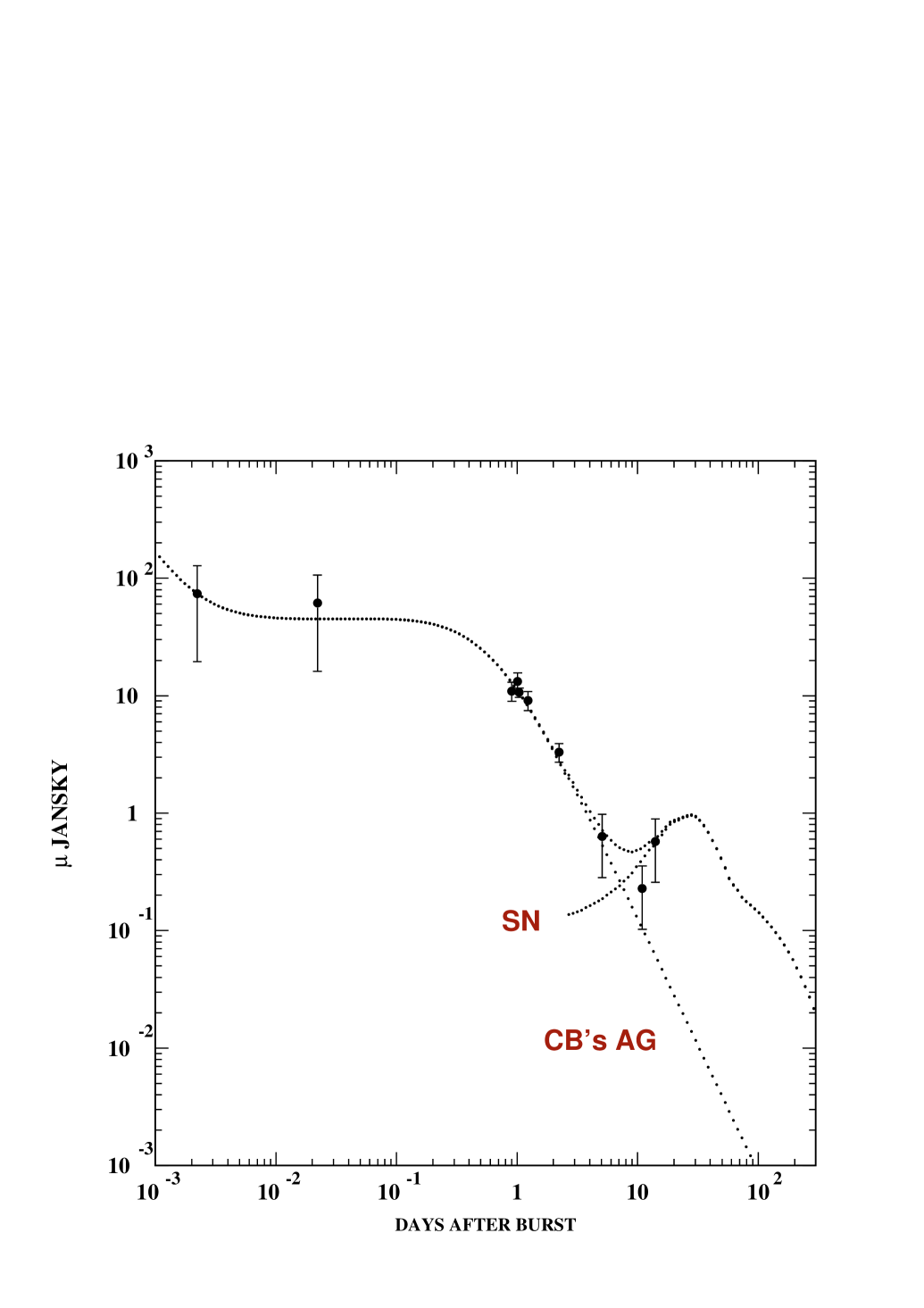
Figure 33: The optical AG of XRF 030723 (Prigozhin et al. 2003; Fox et al. 2003b; Dullighan et al. 2003a,b; Smith et al. 2003; Bond et al. 2003) showing a “rebrightening” 14 days after the XRF that may be due to the contribution of a SN (Fynbo et al. 2003). The first two points have been deduced from the unfiltered measurements of Smith et al. (2003), assuming an early $F_{\nu}\sim\nu^{-0.5}$ (Dado et al. 2003a). All errors were multiplied by a factor 2 to account for cross-calibration uncertainties. The fit is a preview of Dado et al., in preparation. The redshift of the 1998bw-like SN contribution has been adjusted to the normalization of the late-time points; without extinction corrections in the host galaxy or ours, it corresponds to a redshift of $z\sim 0.75$.

Fynbo et al. (2003) have just reported the detection of a rebrightening in the optical AG of XRF 030723 (Fox et al. 2003b; Dullighan et al. 2003a,b; Smith et al. 2003, Bond et al. 2003) 14 days after the XRF (Prigozhin et al. 2003) that may be due to the contribution of a SN. This is demonstrated in Fig. (33) which presents a preview of a CB model fit to the AG of XRF 030723 (Dado et al. in preparation). The normalization of the 1998bw-like SN contribution has been adjusted: without extinction corrections in the host galaxy or ours, it corresponds to a redshift of $z\sim 0.75$. The fitted value of the viewing angle is $\theta\sim 2.8$ mrad, larger than that of any other GRB listed in Table 2, but the very close-by GRB980425.

19 GRBs in the FB models

We discuss here the properties of GRBs in the “standard” FB scenarios, in the same order as we have discussed them in the preceding text on the CB model.

19.1 Polarization

In the most popular variant of the FB models, a GRB pulse is due to synchrotron radiation from the collision of two shells, that generates a magnetic field (e.g. Medvedev & Loeb 1999) and accelerated-electron distribution. Electrons with a power-law distribution $dN_{e}/dE\sim E^{-p}$, immersed in a unidirectional magnetic field, radiate light with a linear polarization, $\Pi=(p+1)/(p+7/3)$ (Rybicki & Lightman 1979). Thus, the polarization of photons from Fermi- or shock-accelerated electron distributions ($2\leq p\leq 3.2$) in a highly ordered magnetic field is typically between 70 and 75%, although even for optimal geometries the polarization cannot exceed $\sim 50\%$ (e.g. Lyutikov et al. 2003).

A disordered magnetic field generated in collisions of shells of a conical jet with a narrow opening angle $\theta\sim\gamma^{-1}<10$ mrad —which is much smaller than those inferred in previous standard FB models (e.g. Waxman 2003a, Frail et al. 2001; Berger et al. 2003; Bloom et al. 2003)— can generate a high polarization if viewed from an angle $\theta\sim 1/\gamma$ (Waxman 2003b), and not from the traditional FB models’ on-axis viewing angle (e.g. Rhoads 1997,1999; Sari, Piran & Halpern 1999; Frail et al. 2001; Berger, Kulkarni and Frail 2003; Bloom et al. 2003). But the light curve of GRB 020106 has many pulses, requiring in a FB model a variety of values of $\gamma$ for the colliding and merged shells. With these varying $\gamma$ values and a fixed observer’s angle, it is quite difficult to imagine how the polarization, integrated over pulses, can be as high as the $80\pm 20\%$ value observed by Coburn and Boggs (2003) in this GRB.

To date, the most detailed FB analysis of the polarization of GRB 021206 is that of Nakar, Piran & Waxman (2003). They find that, by adequately maximizing all effects, and for a single value of the Lorentz factor of a merged shell, they can raise the polarization to 45–50%, significantly below the observation. This requires a magnetic field structure which is both random (to accelerate the synchrotron-emitting electrons) and uniform in space and time (to give rise to the polarization). Alternatively, a model is considered in which the magnetic field is uniform over a small region observed at the edge of the jet. This model requires a large amount of fine-tuning, between the observational angle, the jet opening angle, the inverse of the Lorentz factors of the various merged shells, the Lorentz factors themselves (which must be very similar for the many different merged shells giving rise to the GRB) and the polarization direction of the emission from each shell. But fine-tunings and exceptional cases are the rule in the FB models, not the exception.

The conclusion we would extract from the above is that the FB models where GRBs are produced by synchrotron radiation cannot accommodate a significant GRB polarization: they are ruled out by the large polarization measured by Coburn and Boggs (2003) in GRB 021206.

In one of its multitude of variants, a “fireball” model was studied in which a relativistic wind blowing in a funnel within a star would generate a GRB by ICS off the photons emanating from the funnel’s walls (Ghisellini et al. 2000). The authors noticed that, for a large $\gamma$, the characteristic GRB energies could be explained (Shaviv & Dar 1995); but —perhaps because at the time fireball ejecta were still considered to be broad and to point at the observer— they overlooked the crucial prediction of Shaviv and Dar: a large polarization at the most probable viewing angles $\theta\sim 1/\gamma$.

19.2 Typical energies

In the FB models, the typical energy of GRB photons is given by a combination of parameters that have no reason to conspire to yield the very narrow observed range (e.g. Ghisellini 2001). But it has been argued (Waxman 2003a) that this parameter combination can be rewritten as:

$$E=(1\,{\rm MeV})\;\xi_{B}^{1/2}\,\xi_{e}^{3/2}\;\left(L_{{}_{GRB}}\over 10^{52}\,{\rm erg\,s^{-1}}\right)^{1/6}\;\left({10^{-2}\,{\rm s}\over\Delta t}\right)^{2/3},$$ (68)

where $\xi_{B}$ and $\xi_{e}$ are efficiencies for transforming collisional energy to magnetic and accelerated-electron energies, $L_{{}_{GRB}}$ is the GRB’s luminosity and $\Delta t$ is the scale of GRB variability. The problem with this argument, it appears to us, is in the use of a fixed, universal time scale $\Delta t=10^{-2}$ s. Attributing a fixed variability scale to all GRBs —particularly the dominant fraction without significant narrow spikes— yields the desired result, but seems to be unwarranted. If the more typical variability scale $\Delta t=1$ s were to be used, Eq. (68) would fail by over an order of magnitude. Moreover, for individual GRBs, the correlation between energy and variability implied by (our reading of) Eq. (68) is not observed. Finally, it is not clear how Eq. (68) explains a narrow spread of observed $E$ values. The CB-model’s prediction for $E$ and its distribution, discussed in Section 6, seem to us to be more satisfactory.

19.3 The width of a pulse

In the FB models, there is no particular reason for the width and the total energy of a typical GRB pulse to be what they are, these results must be imposed by fiat: adequate choices of the relevant parameter combinations. Reviews of the subject, such as those of Piran (2000), Mészáros (2002), Hurley et al. (2002) and Waxman (2003b), do not discuss these points, for which the CB-model predictions are given by Eqs. (23) and (26).

19.4 The shape of a pulse

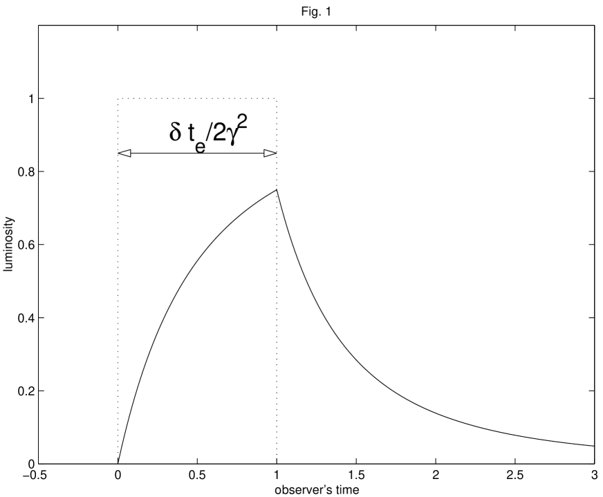
Figure 34: The shape of the luminosity, $E\,dN/dt$, of a GRB in an FB model (Kobayashi et al. 1997).

An example of the shape of a pulse in an FB model is given in Fig. (34), from Kobayashi, Piran and Sari (1997). The combination of parameters determining the rise-time must be tuned to give the observed range of results. The result in Fig. (34) is for the pulse’s luminosity evolution, $E\,dN/dt$, not its $\gamma$-ray number evolution. The result for the latter initially rises as $dN/dt\propto t$ and declines after the discontinuity as $dN/dt\propto 1/t$, in disagreement with observations.

19.5 Spectral shapes

The distribution of values of $\alpha$ and $\beta$ extracted from fits to the GRB data peak close to the values predicted in the CB model $\alpha\approx 1$, $\beta\approx 2.1$. In the FB models, wherein synchrotron radiation is responsible for the GRB emission, the observed $\beta$ can be accommodated, but not the results for $\alpha$: the “synchrotron limit” spectrum (Katz 1994a) corresponds to $\alpha=2/3$; some 10–15% of bursts are harder than that (Preece et al. 1998). Even worse, the electron cooling times are very short, and the resulting synchrotron spectrum should have $\alpha=3/2$, the overwhelming majority of GRB spectra being harder than that. This is occasionally admitted to be an unsurmountable problem, as all known alternatives —synchrotron self-absorption, a smooth cutoff of the low-energy electron distribution, an anisotropic electron distribution with a small mean pitch angle, unsaturated thermal comptonization, Compton drag, synchrotron self-Compton, and the incidence of instrumental effects, are all equally problematic (e.g. Liang 1997; Ghisellini & Celotti 1998; Ghisellini, Celotti & Lazzati 1999; Ghisellini 2001; Preece et al. 2002; Ghirlanda, Celotti & Ghisellini 2002).

19.6 Time–energy correlations

The correlations between time and energy in a GRB pulse —expected on very simple grounds in the CB model— coincide with the ones observed. We are not aware of a similar conclusion within the FB models, as reviews of the subject, such as those of Piran (2000), Mészáros (2002), Hurley et al. (2002) and Waxman 2003b do not discuss this point. The only exception is the correlation $\Delta t\propto E^{-1/2}$ of Eq. (56), obtained in an FB model by Kazanas, Titarchuk and Hua (1998). But this correlation requires a very slow cooling process, implying magnetic fields orders of magnitude smaller than the ones required to accommodate the large observed GRB fluxes. Since the field cannot be simultaneously large and small, Wu & Fenimore (2000) conclude that the agreement with observation (Fenimore et al. 1995, Norris et al. 1996) is a mere coincidence.

19.7 GRB progenitors

The nature of the progenitors of GRBs is, in the FB models, undecided. In Hurley et al. (2002), as in innumerable other instances, the bursts possibly associated with SNe may be of a special class, exactly the opposite of what all GRBs are in the CB model.

From our outsiders’ perspective, as we just argued, the FB models have very serious difficulties accommodating the observations of GRBs.

20 Conclusions and discussion

We have shown how simply and successfully the CB model explains the bulk of the properties of the $\gamma$-rays of GRBs. The key is simple: ICS of the circumburst “ambient” light by the electrons in a CB. We have commented on how unpredictive the FB models are regarding GRBs, their only robust predictions being that of the power behaviour of the $\gamma$-ray spectrum, which fails —unless magnetic fields and the ensuing electron cooling times can be both long and short— and the polarization of the GRBs, which should be tiny (e.g. Medvedev & Loeb) —unless magnetic fields can be both ordered and disordered, or the shells’ Lorentz factors, magnetic-field orientations, opening and viewing angles are all eagerly fine-tuned “just so” (Ghisellini 2003, Nakar et al. 2003). For the GRB AGs, briefly discussed in Appendix II, the situation is similar: the CB model does an excellent job, while the FB models, which are more predictive for AGs than they are for the GRBs themselves, are also more often in disagreement with the observations.

From an insider’s perspective, an asset of the study that we have presented here is the unassailability of its inputs. The properties of the CBs originating GRBs —such as their very substance— are borrowed from those of other CBs observed in nature. The properties of the ambient light that the CBs scatter to GRB energies are also based on observations. Although these inputs cannot be said to emanate from first principles, they are solid. Given these phenomenological inputs, the rest of the ingredients are not in doubt: the fundamental electrodynamics on which the expected spectrum of accelerated electrons within a CB is based, and Compton scattering, one of the most relevant processes in cosmology and astrophysics, and the “Eve” of all particle-physics processes.

Seen from our outsiders’ perspective, the FB models look like a baroque and continuously buttressed edifice. This is not to say that these models have not recently progressed in the direction that we consider correct: that of espousing features of the CB model. What used to be vices have become fashions (Seneca, ${\cal{O}}(30)$ C.E.):

• From the 8^th of April, 2003, the discovery (Garnavich et al. 2003b, Stanek et al. 2003) of SN2003dh —associated with GRB 030329— has transformed the GRB association with fairly unconventional SNe from a minor and doubtful issue (e.g. Hurley et al. 2002; Waxman 2003a) into something crucial that everybody always knew. This association is the basis of the CB model; this SN, its properties and the date of its discovery (that is, the time when the predicted AG would no longer overwhelm the SN signal) were foretold in the CB model (Dado et al. 2003f). The history of the GRB/SN association is reviewed in Appendix III.

• Following the CB model (Dar & De Rújula 2000a,b; Dado et al. 2002a) the observer’s angle, once upon a time set to zero by fiat in the FM model (e.g. Rhoads 1997, 1999; Sari et al. 1999; Kumar & Panaitescu 2000; Frail et al. 2001; Moderski, Sikora & Bulik 2000; Panaitescu & Kumar 2001; Kumar & Panaitescu 2001: Berger et al. 2003; Bloom et al. 2003) is gaining a non-negligible role (e.g. Rossi, Lazzati & Rees 2002; Granot et al. 2002; Zhang & Mészáros 2002; Panaitescu & Kumar 2003; Salmonson 2003). In the CB model only this angle plays a role, the jet opening angle, $\theta_{v}=\beta_{s}/(\sqrt{3}\,\gamma)$, is smaller than the boosted-light opening angle $1/\gamma$, and its effects can be neglected. In the AG phase, as the CBs cease to expand, $\theta_{v}\to 0$.

• The ejecta’s angular spread has progressively diminished from an original $4\,\pi$ solid angle, to a jet opening angle of tens of degrees (Frail et al. 2001), to $\theta_{v}=10$ mrad (Waxman 2003a). This last value, for a typical FB model’s $\gamma=100$, is getting dangerously close to being negligible relative to $1/\gamma$.

• The correlations discussed in Dar & De Rújula (2000b) and in Section 13 (but not those of Fig. (11) and Section 12) should be approximately valid for any jets seen off-axis, as it is beginning to be realized (e.g. Rossi, Lazzati & Rees 2002; Granot et al. 2002; Zhang & Mészáros 2002; Panaitescu & Kumar 2003; Salmonson 2003; Waxman 2003b; Perna, Sari & Frail 2003; Yamazaki, Yonetoku & Nakamura 2003). No doubt that these correlations will soon be fully exploited as a success of forthcoming off-axis FB models.

• With their current, very small $\theta_{v}$ values, GRBs, once systematically publicized as “the biggest explosions after the Big Bang”, have become a small fraction of the energy budget of a conventional SN, that is, what they always were in the CB model.

The FB-models’ ejected shells have lost the elegance of a sphere to become rather contrived, very thin and laterally-small waffles, racing along a radial track, and emitting GRB photons as they bang against one another —like clanging chads. The mystery-clad “generic fireballs”, with their spherical innuendos and their unconventional composition ($e^{+}e^{-}$ pairs) fit —rather uncomfortably— into the centre of a fairly conventional exploding star.

The CB model may of course be wrong, but it is successful. It is not at all inconceivable that the FB models may continue to incorporate and “standardize” other aspects of the CB model. Three large stumbling blocks lie along this path. One is the substance of which the FB-models’ ejecta are made: a delicately baryon-loaded (that is, highly fined-tuned) plasma of $e^{+}e^{-}$ pairs. Such a fancy substance may not be so difficult to forsake, in comparison with good old ordinary matter. Another hindrance is synchrotron emission, the traditional GRB-generating mechanism in most FB models. But then, synchrotron and Compton scattering are the same process: off virtual or real photons. The main obstacle may be the magic wand of FB models: shocks. If and when these obstacles are overcome, the fireballs may turn out to have always been cannonballs for, after all, in the CB model,… SNe fire balls.

The phenomenological simplicity of the CB model may make long and short GRBs, as well as XRFs, useful in the study of SNe and of the cosmos at large $z$. Perhaps Type Ia SNe, as we have briefly discussed, are the originators of short-duration GRBs, in which case the spotting of these SNe may be greatly facilitated. The association of long-duration GRBs with core-collapse SNe will, at the very least, help in ascertaining the death rate of massive stars at large $z$, to which their birth rate is indisputably proportional.

One serious drawback of the CB model is that it makes GRBs become very uninteresting, in comparison with what they used to be: one of the biggest mysteries of astrophysics and the biggest of explosions of all times (the Big Bang, in our current understanding of it, was not an explosion in any sensible sense). Fortunately, and independently of the “peripheral” GRB- and AG-generating physics, the biggest conundrum remains: How does a SN manage to sprout mighty jets? In the CB model the guidance along this path is better than simulations: the CBs responsible for GRBs are akin to the increasingly well–studied ejecta of quasars and microquasars. The CB model tends bridges to other observational fields as well: cosmic rays (Dar & Plaga 1999), the gamma background radiation (Dar & De Rújula 2001), cooling flows (Colafrancesco, Dar & De Rújula 2003) and, perhaps, astrobiology (Dar & De Rújula 2002).

The CB model is very predictive, so that its limitations may be readily found. One example might be that of the superluminal motion of CBs in the sky. This motion may be observable, indirectly via scintillations (Dado et al. 2003a), directly in the case of GRBs at sufficiently small $z$ (Dar & De Rújula 2000a), or even independently of a GRB signal in the case of truly close-by SNe, such as SN1987A, whose two opposite CB jets are shown in Fig. (36). So far the only putative problem the CB model has encountered has to do with the superluminal motion of the CBs of GRB 030329. Indeed, we learned by reading the e-version of NYT 030529 (the New York Times of that date, in GRB’s parlance) that, according to Dale Frail “[Our observations] are sufficient to rule out predictions of the cannonball model”. The predictions of a model cannot be ruled out, but a (good) model can… if its predictions are decisively proved wrong. We are only now beginning to have sufficient data on the radio AG of this GRB to make these predictions sufficiently specific. When that is done, and when we see the data, we shall be able to ascertain whether or not, concerning the death of the CB model, we are —or we are not— led to reminisce a similar announcement: that of the death of Mark Twain.

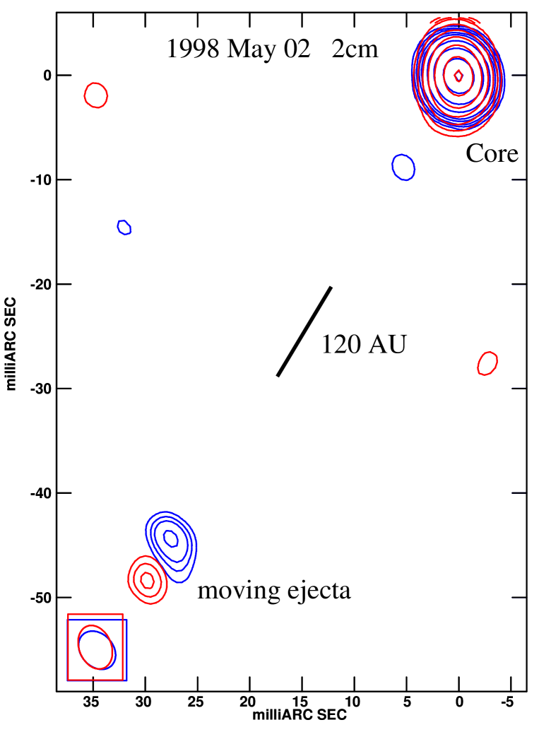
Figure 35: The May 1998 VLBA 2-cm radio images of the microquasar GRS 1915+105 and the superluminal CB it ejected $67\pm 7$ h before, at 75 AU resolution. Contours are at $2$, 2.3, 4, 6, 8, 16, 32, 64, and 96% of the peak intensity. The blue and red contours show time-resolved images 4.5 h apart.

Acknowledgements: This research was supported in part by the Helen Asher Space Research Fund for research at the Technion. Comments and suggestions by Shlomo Dado and Rainer Plaga are gratefully acknowledged. We are thankful to Felix Mirabel and Mario Hamuy for sending us Figs. (35) and (32), respectively. One of us, Arnon Dar, is also grateful for the hospitality extended to him at the CERN Theory Division.

21 Appendix I: Collisionless shocks or shockless collisions?

Shocks are a fundamental building-block of the FB models, while in the CB model they play no role whatsoever in the generation of GRBs or their AGs. The substance of the shells responsible for GRBs is, in the FB models, an $e^{+}e^{-}$ plasma with a tuned “baryon load”. The substance of CBs is ordinary matter. We comment here on the observational situation regarding these two issues in the realm of the other relativistic jets observed in nature: the ejecta of quasars and microquasars.

According to the standard lore, the impact of a moving shell on the ISM produces a forward shock in the ISM and a reverse shock in the shell. For non-relativistic shocks, such as those generated by the expansion of SN shells into the ISM, the temperature of the particles behind the shocks is $T_{i}\sim(3/16)\,m_{i}\,v_{s}^{2}$, where $v_{s}$ is the velocity of the forward or reverse shock in the ISM’s or shell’s rest frame, respectively (e.g. McKee & Hollenback, 1980). This relation is not well satisfied in young SN remnants. A typical shock velocity of 4000 km s^-1 should give rise to a plasma temperature of 19 keV (e.g. Hughes et al. 2000). The observed temperatures are in all cases smaller than 5 keV. Moreover, high resolution spectral measurements show that the X-ray line widths of metals in the reverse-shock region do not have the mass dependence expected for thermal widths (Vink et al. 2003).

The above unsuccessful fluid-dynamic picture has been adopted in the relativistic FB models of GRBs (Rees & Mészáros 1992, 1994; Paczynski & Rhoads 1993; Katz 1994a,b; Mészáros & Rees 1997; Waxman 1997a,b; Sari, Piran & Narayan 1998), using the Blandford–McKee (1976) formalism for relativistic shocks. In this picture, the “kinetic” temperatures of the random motion of the protons and of the electrons behind relativistic shocks rise to $T_{p}\sim\gamma\,m_{p}\,c^{2}$ and $T_{e}\sim\gamma\,m_{e}\,c^{2}$ (e.g. Waxman 1997a,b). The forward shocks become promptly relativistic, and after $\sim\!1$ s, when the shell has swept up sufficient ISM, so do the reverse ones (e.g. Wang, Loeb, & Waxman 2002) and so does the “temperature” of the particles in the shell’s rest frame.

Applied to the relativistic jets launched by quasars and microquasars, this formalism implies that very high temperatures are produced in the jets by reverse shocks. This conflicts with the observations of atomic-line emission from the jets. The velocity of the CBs repeatedly ejected from the microquasar SS433, for instance, is $\sim$ 0.26c (Margon 1984). The spatially resolved optical (e.g. Eikenberry et al. 2001), UV (e.g. Gies et al. 2002), and X-ray spectra (Marshall, Canizares & Schultz 2002; Migliari, Fender & Méndez 2002; Namiki et al. 2003) of the approaching and receding CBs show blue- and red-shifted emission lines of H, He, metals and heavy elements. In particular, the Balmer lines and other forbidden lines indicate that the ambient plasma temperature is less than 1 eV, i.e. a few orders of magnitude smaller than expected from a reverse shock (e.g. McKee & Hollenback 1980).

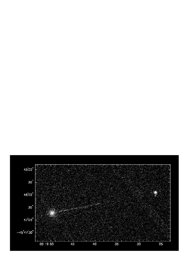
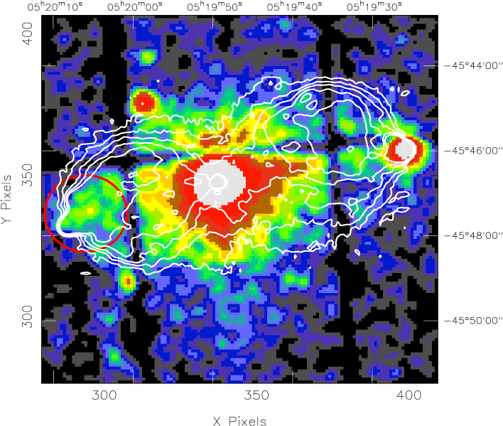
Figure 37: Upper panel: Chandra X-ray image of the radio galaxy Pictor A (Wilson, Young & Shopbell 2001), showing a non-expanding jet that emanates from the centre of the galaxy and extends across 360 thousand light years towards a brilliant hot spot at least 800 thousand light years away from where the jet originates. Lower panel: XMM/p-n image of Pictor A in the 0.2–12 keV energy interval, centred at the position of the leftmost spot in the upper panel, and superimposed on the radio contours from a 1.4 GHz radio VLA map (Grandi et al. 2003).

One of the arguments often brandished against the CB model is that CBs travelling in the ISM should produce bow shocks impeding the penetration of further ISM particles into them (e.g. A. Loeb, private communication). A bow shock is created by a bullet travelling in air because neither air nor the bullet are collisionless, nor relativistic (a beam of high-energy particles does penetrate lead targets). A collisionless bow shock is made by the low-energy protons emanating from the Sun as they encounter the Earth’s extensive (i.e. bipolar) magnetic field. But high-energy protons do reach the atmosphere, and so do most protons in the polar regions where the field is weak, witness the aurora. The ISM protons and electrons impinging on a CB do it with a very large relative Lorentz factor, and the magnetic field of a CB is chaotic: multipolar and of very short range outside the CB. Lastly, bow shocks are not observed in the CBs emitted by quasars (e.g. Pictor A in Fig. (37); M87: Harris et al. 2003; 3C273: Sambruna et al. 2001), microquasars (e.g. GRS 1915+105: Dhawan, Mirabel & Rodriguez 2000, XTE J1550-564: Corbel et al. 2002), and pulsars (e.g. Vela: Pavlov et al. 2003). In Fig. (35) we reproduce the May 1998 VLBA 2-cm radio images of the microquasar GRS 1915+105 and the superluminal CB it ejected $67\pm 7$ h before, at 75 AU resolution. No bow shocks are observed, neither in this image nor in higher resolution (2.5–7.5 AU) images, which are the most spatially resolved images of a relativistic jet ever obtained (Dhawan et al. 2000).

Strong X-ray emission lines with large equivalent widths and Doppler factors $\delta\sim\!2$ to 3, interpreted as Fe ${\rm K\alpha}$ lines, were found with the ASCA (e.g. Yaqoob et al. 1999) and Chandra (Wang et al. 2003) satellites in radio-loud quasars. Such emission cannot be produced if the Fe kinetic temperature in the quasar’s jets is well above a few tens of keV. Yet, if reverse shocks are generated in these jets by their interaction with the ISM of the host galaxy, the observed $\delta$ values imply relativistic temperatures.

The observed atomic lines from the relativistic jets of quasars and microquasars imply that the jets are made of ordinary atomic matter and not of $e^{+}e^{-}$ pairs. The lines can be emitted from relatively cold ordinary matter, by collisional excitation of the jet atoms by the incoming ISM particles (as in Röntgen’s experiment). The observed non-thermal line widths may be due to velocity dispersion of the motion of matter in the CBs of the jets.

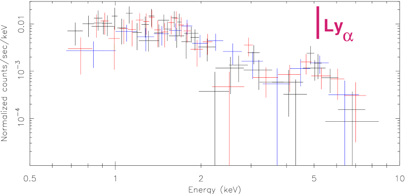
Figure 38: The X-ray spectrum of GRB 970828 in the intermediate time-period in which a putative line feature was observed (Yoshida et al. 2001). The vertical line is at the position (at that time) predicted in the CB model for the highly Doppler-boosted Hydrogen $\rm Ly\alpha$ transition (Dado et al. 2003b).

In the CB model the CBs responsible for GRBs are assumed to be made of ordinary matter, like the CBs emitted by quasars and microquasars. Even after a CB is no longer significantly heated by hadronic collisions with the SN shell and the wind, it is kept partially ionized by synchrotron self-absorption (Dado et al. 2003a,b). Its atoms should emit light at characteristic line energies $E_{l}$, seen by an observer at $E_{l}\,\delta(t)/(1+z)$, with $\delta(t)$ the Doppler factor at the observation time $t$, a decreasing function of time, given the fact that $\gamma(t)$ diminishes, in the way described by Eq. (65), as the CB ploughs through the ISM (a significant effect at the time of X-ray AG observations, insignificant in the GRB phase). For GRBs with measured AGs, the CB model fit to the AG determines $\delta(t)$, so that the line positions can be predicted. There are marginal but intriguing observations of X-ray lines in GRB AGs (Piro et al. 1998, 2000; Antonelli et al. 2000; Yoshida et al. 2001; Reeves et al. 2002; Watson et al. 2002a,b; Butler et al. 2003; Watson et al. 2003). All of these putative observed lines are, auspiciously, at boosted line energies expected in the CB model. An example of the comparison of the predicted boosted Ly$\alpha$ line and the observations is given in Fig. (38).

22 Appendix II: AGs in the FB models and in the CB model

Unlike the FB models, the CB model offers a very simple, successful and complete description of the AGs of all GRBs of known redshift, including the all-important GRB 980425, associated with SN1998bw (Dar & De Rújula 2000a, Dado et al. 2003a).

One key ingredient of the CB model in the AG phase is that, we contend, CBs stop expanding after minutes of (observer’s) time, to reach a stable situation in which (in the CB’s rest system) their internal magnetic pressure is balanced by the inward pressure of the ISM electrons and nuclei that they gather, isotropize and re-emit into the ISM. The re-emitted particles, accelerated in the CB by a single “collisionless elastic scattering” to energies up to $2\,\gamma^{2}\,M\,c^{2}$ (and by multiple scatterings to higher energies) subsequently constitute the cosmic rays of the GRBs’ host galaxy.

To quote one of our referees: “The majority of the [GRB] community believes this [CB] model is wrong, as the jet should spread”; the emphasis is ours. In Fig. (37) we show, in the upper panel, a Chandra X-ray image of the radio Galaxy Pictor A, showing a non-expanding jet that emanates from the centre of the galaxy and extends across some 360 thousand light years towards a brilliant hot spot at least 800 thousand light years away from where the jet originates (Wilson, Young & Shopbell 2001), and, in the lower panel, an XMM/p-n image of Pictor A in the 0.2–12 keV energy interval, superimposed on the radio contours from a 1.4 GHz radio VLA map (Grandi et al. 2003). What we intend to illustrate with this figure is that uncanningly narrow jets are observed in nature, when looked at the X-ray frequencies at which we see the synchrotron radiation or the Compton up-scattered photons of the cosmic microwave background, emanating from within the CBs. The extensive and somewhat biconical radio emission is, in our interpretation, due to synchrotron radiation by the mentioned cosmic rays in the ambient magnetic field. The hot spot is the place where the jetted CBs finally have lost all of their kinetic energy to cosmic-ray acceleration and, no longer suffering an inwards pressure, they simply expand.

Rather than deciding by fiat that the CB model is wrong, we would conclude that it also offers an explanation for the extremely narrow jets observed at X-ray frequencies, not only in Pictor A, but in more than twenty other quasars, blazars and radio galaxies that were observed with Chandra (Gelbord et al. 2003, Marshall et al. 2003). In several cases the narrow jets were resolved into plasmoids (CBs), such as in M87, Cygnus A and 3C279, or in microquasars such as GRS 1915+105 (Dhawan Mirabel & Rodriguez 2000), XTE J1550-564 (Corbel et al. 2002), 4U 1755-33 (Angelini & White, 2003), and even in pulsars (e.g. Vela: Pavlov et al. 2003).

We cannot compare one to one the analyses of GRB AGs in the FB and CB models, and we shall limit ourselves to a few illustrative examples. In Section 4.3 we mentioned the CB-model interpretation of AGs, with the example of the R-band AG of GRB 021211, shown in Fig. (3). This AG has also been analysed in an FB model (Fox et al. 2003a and references therein). The early AG is attributed to a “reverse shock”, whose fast time decline and normalization are fit to the data. The latter behaviour is, as in other GRBs, not measured at an early time, due to a “forward shock”, whose normalization and time decline are independently fit to the data, with two successive power laws, when a steepening with time (a “break” at a fit break time) is observed. The SN signature at $t>10$ days is not discussed. Moreover the FB model, unlike the CB model, fails to describe the evolution of the radio flux. Fox et al. (2003a) conclude that “the burst may have suffered substantial radiative corrections”. They offer no explicit support (i.e. a comparison of the data and the predictions of such a modified FB model) for their conclusion.

The FB-models’ analysis of the AG of GRB 991208 is more elaborate. Analysing its early broad–band data, Galama et al. (2003) are forced to conclude that “the jet model can account for the observed evolution… provided the jet transition has not been fully completed in the first two weeks after the event”. The predictions of this paper disagree with subsequent radio data, gathered and re-analysed in Galama et al. (2003). This time the conclusions, also unsupported, change to “the relativistic blast-wave entered a non-relativistic expansion phase several months after the burst”. In sharp contrast, the parallel successive analyses of this AG in the CB model —in the same simple terms that describe all other measured AGs— are predictive and successful (Dado et al. 2002a; 2003a,d).

The defence of the FB models in the analysis of AGs is sometimes less vague. An example is GRB 030329, whose light curves for the GRB photon number-count and R-band fluence (along with its CB-model fit) are shown in Figs. (30) and (31). In their FB model analysis, Granot, Nakar & Piran (2003) conclude that the fluctuations in the R-band fluence relative to a smooth curve are best explained by refreshed shocks. The logic of this conclusion is unassailable: fluctuations in the energy output are due to fluctuations in the energy input.

In the CB model, GRBs are less interesting, in that not many of them are —as they are in the FB models— indicative of new effects (ordered magnetic fields, radiative corrections, incomplete jet transitions, non-relativistic expansions, refreshed shocks, to quote only the ones we have mentioned in connection with AGs). The CB model fit to the AG of GRB 030329, shown in Fig. (31), relies on the observation that the GRB light curve is dominated by two clear pulses, or CBs, as shown in Fig. (30), where we have described the two pulses with the naive shape of Eq. (37). The AG is thus fitted (admittedly with similarly unassailable logic) with two distinct CB contributions. Notice that the data determining the properties of one or the other CB are different: before $t\sim 1$ day the AG is overwhelmingly dominated by the first CB, while the later data is overwhelmingly dominated by the second. Naturally, the fit returns very different values for the parameters of the two CBs, with one very significant exception: the observation angles are $\theta_{1}=2.00$ mrad and $\theta_{2}=1.95$ mrad. Values of $\theta$ for other data sets (other GRBs) expand over a much larger range. The chance probability of obtaining $\theta_{1}=\theta_{2}$ to such precision is negligible unless, that is, the CB model has some truth in it (the same “coincidence” takes place for the other GRB with two clear CB contributions, GRB 021004 (Dado et al. 2003c). Incidentally, the prediction of a SN contribution, shown in Fig. (31), was subsequently found to be correct (Stanek et al. 2003).

The FB model has been used, thrice to our knowledge, to predict the late-time evolution of AGs on the basis of the early data: those pertaining to the GRBs 021004, 030226 and 030329. The method was to use the “empirically demonstrated” relation between the total isotropic energy of the GRB and the “break” time, $t_{b}$, at which the AG light curves steepen (Frail et al. 2000; Berger et al. 2003; Bloom et al. 2003) to predict the latter in terms of the former, and to extrapolate the early AG data to later times with the use of a typical steepening at the break. In the case of GRB 021004, Malesani et al. (2003) predicted a break at $t_{b}\sim 13.7$ days. A first break took place at $t_{b}<0.1$ days after burst (Weidinger et al. 2002) and a second one at $t_{b}\sim 5$ days (Holland et al. 2003). For GRB 030226, Rhoads et al. (2003) predicted $t_{b}\sim 10$ days. The observation was $t_{b}\sim 0.8$ days (e.g. Greiner et al. 2003). Finally, for GRB 030329, the expectation (Uemura et al. 2003) was $t_{b}>60$ days, and the observation $t_{b}\sim 0.57$ days (Burenin et al. 2003). So, in each and everyone of these cases the prediction failed by a considerable margin.

Even when applied to the same GRB’s AG, the extraction of $t_{b}$ is problematic. In the case of GRB 020813, for instance, Covino et al. (2003b) extract $t_{b}=0.59\pm 0.03$ days from data in the interval between 3 hours and 4 days, while Li et al. (2003) obtain $t_{b}=0.13\pm 0.03$ days, for data in the 1.7 hours to 1.2 days period. The precision with which the fit values of $t_{b}$ are quoted is impressive, when compared with the difference between the central values.

Frail et al. (2000), Berger et al. (2003) and Bloom et al. (2003) have deduced values of the FB-model’s jet opening angle from the $t_{b}$-values of a sample of GRBs with good AG follow-up and known $z$, and inferred that the “true” $\gamma$-ray energy release in these GRBs is narrowly distributed around $1.3\times 10^{51}$ erg. In view of the fate of other uses of the break-time concept, we do not consider the many-orders-of-magnitude disagreement between this result and that of Eq. (34) to be significant. The CB model relation for the equivalent isotropic energy, Eq. (14), with a very narrow range of ${\cal{E}}^{\prime}_{CB}$ values —and the value of $\delta$ determined in each case by fits to the AG data— is much better satisfied than the FB-model-inspired relation, and this with no exceptions (e.g., Dado et al. 2002a; 2003c,e,f).

The absence of AGs with evidence for a wind-fed circumburst medium is a problem recognized by even the staunchest defenders of the FB models (e.g. Price et al. 2002, Nakar et al. 2003). In the CB model all AGs caught early enough to trace the wind-density profile —GRB 990123, GRB 021004 and GRB 021211, illustrated in Fig. (3)— show an impressive agreement with the very explicit prediction of the theory for the early optical AGs at fixed frequency: $F_{\nu}\propto(n_{e})^{2/3}$ (Dado et al. 2003e).

The wide-band spectrum of AGs in FB models (e.g. Sari, Piran & Narayan 1998) —which paraphrases the theoretical spectrum used to describe synchrotron emission from quasar jets and lobes (e.g. Meisenheimer et al. 1989; Longair 1994)— evolved through a series of papers to its current version (Granot & Sari 2002). This spectrum is extremely complicated: it has a handful of frequency breaks with different time behaviours, which may be ordered in a variety of ways, and must all be fit to the observations. In the CB model, the spectral shape involves no independent parameters other than a single number: an absorption frequency $\nu_{a}$, relevant only in the radio domain (Dado et al. 2003a). This stark contrast does not detract the CB model from working well where the FB models fail (see e.g. Galama et al. 2000b,2003; Dado et al. 2003d).

Two highly relativistic FB-model shells of equal mass $m$ and Lorentz factors $\gamma$ and $\gamma/2$ merge into an object of invariant mass $2\,m\,[1+1/16+{\cal{O}}(1/\gamma^{2})]$: the efficiency for creating new forms of energy is 1/16. The merged object, if colliding with something much more massive and at rest (the ISM), converts all of its kinetic energy into new internal energy. Thus, in the favoured internal–external-shock FB models —and as occasionally recognized (e.g. Ghisellini 2001)— the total energy in a GRB ought to be at least one order of magnitude smaller than that in the AG. The observations are the other way around.

We mentioned in the previous appendix the extremely simple and predictive CB-model interpretation of the X-ray lines allegedly seen in some GRB AGs (Dado et al. 2003b). In the realm of FB models, these lines are attributed to transitions in ionized Fe and other metals. Accommodating them calls for heavy metal envelopes with a large variety of ad-hoc properties and “designer” shapes (for reviews see, for instance, Boettcher 2002; Lazzati 2002). In the CB model the lines do not require any extra assumption, and their positions are predictable.

From our perspective, as we have argued and illustrated with a few examples, the FB models have very serious difficulties in predicting or even accommodating a posteriori the observations of GRB AGs.

23 Appendix III: The GRB/SN association

In Dado et al. 2003f we foretold that on 8 April, 2003 a SN akin to SN1998bw would be bright enough to be discovered spectroscopically as a contribution to the AG of GRB 030329. The spectroscopic discovery of SN2003dh in the AG of GRB 030329 on the expected date, with a luminosity and spectrum remarkably similar to those of SN1998bw (Garnavich et al. 2003b; Stanek et al. 2003), has provided convincing evidence that, undoubtedly, most long-duration GRBs are produced in SN explosions akin to SN 1998bw, as advocated in the CB model (Dar & De Rújula 2000a; Dado et al. 2002a), see Figs. (29,32).

The possible association of GRBs with SN explosions was suggested long before the first observational evidence was serendipitously found. Colgate (1968, 1975) conjectured that the breakout of the shock wave from the stellar surface in a core-collapse SN produces a GRB, but this implied a GRB rate orders of magnitude larger than observed and a GRB from SN1987A which was not detected (Chupp et al. 1987). Dar & Dado (1987) considered the possibility that radiative decay of neutrinos from core-collapse SN explosions would produce GRBs, they used the disparity between the cosmic SN and GRB rates to derive bounds on $\nu$ radiative decay. Goodman, Dar & Nussinov (1987) suggested that $e^{+}e^{-}$ pairs produced by $\nu\,\bar{\nu}$ annihilation in accretion-induced collapses of white dwarfs and/or neutron stars in binary systems, or from neutron-star mergers, may produce GRBs. Yet, the authors found that baryon contamination of the fireball (now known as “baryon-load”) poses a severe problem for this mechanism. Shaviv & Dar (1995) proposed that GRBs may be produced by ICS of light by collimated relativistic jets ejected in the birth of neutron stars and black holes in SN explosions in distant galaxies.

The first evidence for a possible GRB-SN association came from the discovery by Galama et al. (1998) of the very bright SN1998bw, at redshift $z=0.0085$, within the Beppo-SAX error circle around GRB 980425 (Soffitta et al. 1998), whose light curve indicated that the time of explosion was within $-2$ to 0.7 days of the GRB (Iwamoto et al. 1998). This evidence did not fit at all into the framework of the FB model of GRBs. The total equivalent isotropic $\gamma$-ray energy release, $\sim 8\times 10^{47}$ erg, was some 5 orders of magnitude smaller than that expected from a “classical” GRB at $z=0.0085$. The FB community concluded that either SN1998bw and GRB 980425 were not physically connected or that, if they were, they represented a new subclass of rare events (e.g. Bloom et al. 1998; Norris, Bonnel & Watanabe 1998; Hurley et al. 2002). These would be associated with what Iwamoto et al. (1998) and Paczynski (1999) called “hypernovae”: super-energetic explosions with kinetic energy exceeding $10^{52}$ erg, as was inferred for SN1998bw from its high expansion velocity and luminosity (Patat et al. 2001), and from the very strong radio emission from its direction (Kulkarni et al. 1998). Hofflich, Wheeler & Wang (1999) retorted that core-collapse SNe may not be spherical-symmetric and the inferred kinetic energy of SN1998bw could have been overestimated.

SN1998bw was initially classified as Type Ib (Sadler et al. 1998) and later as a peculiar Type Ic (Filippenko 1998; Patat and Piemonte 1998, Patat et al. 2001). Its discovery initiated intensive searches of positional and approximate temporal coincidence between GRBs and SN explosions (e.g. Kippen et al. 1998), in particular Type Ib and Ic SNe (Woosley, Eastman & Schmidt 1999). The search yielded two inconclusive associations, one of them, discussed in Section 17, between the peculiar Type II SN1997cy, at $z=0.063$, and the short-duration ($\sim 0.2$ s) GRB 970514 (Germany et al. 2000) and another one between the Type Ic SN1999E at $z=0.0261$ and the long-duration GRB 980910 (Thorsett & Hogg 1999; Rigon et al. 2003).

SNe of Types II/Ib/Ic are far from being standard candles. But if they are axially as opposed to spherically symmetric —as they would be if a fair fraction of them emitted bipolar jets— much of their diversity could be due to the angle from which we see them. Exploiting this possibility to its extreme, i.e. using SN1998bw as an ansatz standard candle, Dar (1999a) suggested that the AGs of all GRBs may contain a contribution from a SN akin to SN1998bw, placed at the GRB’s position. Dar & Plaga (1999) and Dar & De Rújula (2000) advocated the view that most core-collapse SN explosions may result in GRBs.

Possible evidence for a SN1998bw-like contribution to a GRB AG (Dar 1999a; Castro-Tirado & Gorosabel 1999) was first found by Bloom et al. (1999) for GRB 980326, but its unknown redshift prevented a definite conclusion. The AG of GRB 970228 (located at redshift $\rm z=0.695$) appears to be overtaken by a light curve akin to that of SN1998bw (located at $\rm z=0.0085$), when properly scaled by their differing redshifts (Dar 1999b; Reichart 1999; Galama et al. 2000a). Possible evidence of similar associations was found for GRB 990712 (Bjornsson et al. 2001; Dado et al. 2002a), GRB 980703 (Holland et al. 2001; Dado et al. 2002a), GRB 000418 (Dar & De Rújula 2000a; Dado, Dar & De Rújula 2000a), GRB 991208 (Castro-Tirado et al. 2001; Dado, Dar & De Rújula 2002a), GRB 970508 (Sokolov 2001; Dado et al. 2002a), GRB 000911 (Lazzati et al. 2001; Dado et al. 2002 unpublished), GRB 010921 (Dado, Dar & De Rújula 2002d), GRB 011121 (Dado et al. 2002b; Garnavich et al. 2003; Bloom et al. 2002) GRB 020405 (Price et al. 2002; Dado et al. 2003b), and GRB 021211 (Dado et al. 2003e).

In the absence of precise spectroscopic information on late-time AGs, the identification of a SN contribution requires a reliable model for extrapolating the early-time AG to later times, as well as reliable information on the extinction in the host galaxy. Using the CB model, Dado et al. (2002a) have shown that the optical AGs of all GRBs with known redshift $z<1.1$ contain either evidence for a SN1998bw-like contribution (in the GRBs 980425, 970228, 990712, 991208, 000911, 012111, 010405, 021211 and 030329) or clear hints (in the cases of GRBs 970508, 980613, 980703 000418 and 010921, for which the scarcity of data and/or the lack of spectral information and multi-colour photometry and/or uncertain extinction in the host galaxy prevented a firmer conclusion). In the more distant GRBs ($z>1.1$) the ansatz standard candle could not be seen, and it was not seen.

Naturally, truly “standard candles” do not exist, but SN1998bw made such a good job at it that it gave us enough confidence to predict the SN contribution to the late-time afterglow of all recent cases of early detection of the AGs of near-by GRBs (000911, 010921, 010405, 012111, 021211 and 030329). In all these cases, from a fit to the early-time afterglow, the CB model correctly predicted the late-time appearance of a SN in the late-time colour light curves (Dado et al. 2002b,c; 2003e,f). Besides the GRB 980425–SN1998bw pair, the most convincing GRB/SN associations were provided by the recent spectroscopic discoveries of a SN in the optical afterglows of GRBs 030329 (Stanek et al. 2003; Hjorth et al. 2003) and GRB 021211 (Della Valle et al. 2003).

The observability of a SN signal depends on the size of the AG “background”. The predictions of “the future” of AGs reviewed in the previuos paragraph are in stark contrast with the corresponding ones made in the realm of FM models, not only at optical frequencies, but also in the radio (as we discussed in the previous Appendix in connection with AG “break” times, and with GRB 991208; respectively) and in the X-ray domain (e.g., compare the observations of Pian et al. 2003 with the predictions of Dado et al. 2002a; 2003a).

Additional indirect evidence relating long-duration GRBs to core-collapse SNe follows from the association of well localized GRBs with massive star-formation regions in their host galaxies (e.g. Paczynski 1998; Fruchter et al. 1999; Holland & Hjorth 1999; Bloom, Kulkarni & Djorgovsky 2002), where most of these SNe are expected to take place, as well as from the statistics of the types of galaxies that host GRBs (e.g. Hogg and Fruchter 1999).

A model that explicitely links GRBs to SNe is the “supranova” model of Vietri & Stella (1999), in which it is assumed that a GRB occurs weeks or months after the SN. This is inconsistent with the measured delays between GRB times and the estimated time at which their observed associated SNe exploded.

In an abridged version of the long history of the GRB/SN association we have presented, Stanek et al. (2003b) and Hjorth et al. (2003) attribute its theoretical prediction to Woosley (1993a,b). In these papers, it is proposed that GRBs are produced by the collapse of very massive stars into a black holes in failed SNe: implosions that do not result in a SN signal. The “collapsar” model —wherein massive stars collapse into black holes in Type Ib or Ic SN events— was proposed by MacFadyen & Woosley (1998, 1999) and by Woosley & MacFadyen (1999) after the discovery of the association between GRB980425 and SN1998bw. This latter idea —in the realm of the CB model and for quite ordinary SNe, as opposed to hypothetical supranovae, collapsars or hypernovae— is, in our opinion, the only one still alive and doing well.

Table 1: Typical parameters of a CB^a, the early SN luminosity, the “wind” and the “ambient light”.

$$\begin{array}[]{ p{0.13\linewidth}l p{0.28\linewidth}l}\hline\cr\vskip 3.0pt plus 1.0pt minus 1.0pt\cr Parameter&\rm Value&Definition\\ \vskip 3.0pt plus 1.0pt minus 1.0pt\cr\hline\cr\vskip 3.0pt plus 1.0pt minus 1.0pt\cr$\;\;\;\;\;\>\;\gamma$&\approx 10^{3}&Lorentz factor\\ $\;\;\;\;\;\>\;\theta$&\sim 10^{-3}&Observer's viewing angle\\ $\;\;\;\;\;\>\;\delta$&\sim 10^{3}&Doppler factor\\ $\;\;\;\;\;\>\;\beta_{s}$&\sim 1&Initial expansion velocity\\ $\;\;\;\;\;\>\;N_{{}_{B}}$&{\cal{O}}(10^{50})&Baryon number\\ $\;\;\;\;\;\>\;E_{i}$&\sim 1\;{\rm eV}&Ambient-light energy\\ $\;\;\;\;\;\>\;L_{{}_{SN}}$&\sim 5\times 10^{42}\;{\rm erg\,s^{-1}}&Early SN luminosity\\ $\;\;\;\;\;\>\;\rho\,r^{2}$&\sim 10^{16}\;{\rm g\,cm^{-1}}&Wind's surface density\\ $\;\;\;\;\;\>\;{\cal{E}}^{\prime}_{{}_{CB}}$&\approx 10^{44}\;{\rm erg}&Rest radiation energy\\ \hline\cr\hline\cr\end{array}$$

• Comments: The various symbols reflect the spread of the fitted values for CBs, ranging from “$\approx$” for a narrow distribution to “${\cal{O}}$” for a rough estimate. The parameters $\delta$ and ${\cal{E}}^{\prime}_{{}_{CB}}$ are deduced, not used as inputs.

Table 2: GRBs of known redshift for which we have performed a CB-model fit to the AG. Listed are redshifts, viewing angles $\theta$ (in mrad), initial Lorentz and Doppler factors $\gamma$ and $\delta$, and the quantity $\sigma$ defined in Eq. (21). Two AGs were fitted with two CBs.

GRB	$z$	$\theta$	$\gamma$	$\delta$	$\gamma\,\theta$	$\sigma$
970228	0.695	1.69	540	590	0.91	0.376
970508	0.835	2.51	1123	325	2.82	0.398
970828	0.958	0.86	1153	1163	1.00	1.370
971214	3.418	0.71	999	1331	0.71	0.600
980425	0.0085	7.83	495	62	3.88	0.060
980703	0.966	0.95	779	1004	0.74	0.795
990123	1.600	0.46	1204	1630	0.55	1.509
990510	1.619	0.26	1009	1889	0.26	1.455
990712	0.434	0.75	948	1259	0.71	1.664
991208	0.700	0.11	1034	2041	0.11	2.482
991216	1.020	0.40	906	1598	0.36	1.433
000131	4.500	0.10	1200	2365	0.12	1.032
000301c	2.040	2.32	1061	300	2.46	0.209
000418	1.119	2.06	1241	329	2.55	0.385
000911	1.060	0.29	800	1516	0.23	1.177
000926	2.066	0.74	787	1521	0.58	0.781
010222	1.474	0.47	1178	1813	0.55	1.727
010921	0.451	0.15	1013	1980	0.15	2.765
011121	0.360	0.10	1222	2405	0.12	4.322
011211	2.141	1.16	824	862	0.95	0.452
020405	0.69	0.42	645	1201	0.27	0.917
020813	1.225	0.58	1128	1587	0.65	1.558
021004	2.330	1.47	1403	542	2.06	0.457
	2.330	1.47	1259	576	1.85	0.436
021211	1.006	1.76	262	431	0.48	0.113
030226	1.989	1.14	824	876	0.94	0.482
030329	0.168	2.25	1652	222	3.73	0.629
	0.168	2.10	1037	362	2.18	0.644

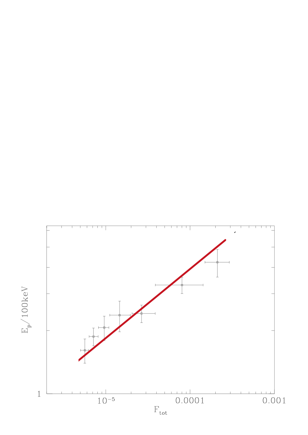
Figure 21: Averaged peak energy, $E_{p}$, versus total fluence, $F_{tot}$, in bins containing 20 GRBs of similar fluence (Lloyd et al. 2000). The line is the prediction of Eq. (59).

Figure 24: Observed GRB duration ($t_{90}$) and total energy fluence in the 7-400 keV band of 35 GRBs that were measured by HETE II (Barraud et al. 2003). The theoretical continuous line is the average trend expected in CB model for the width of the individual pulses. The theoretical dashed line is the expectation for the time intervals between pulses.

Figure 25: The luminosity–variability correlation. The data analysis is from Reichart et al. (2001). The line is the prediction of Eq. (61), applied to complete GRBs, rather than single peaks.

Figure 26: The peak energy–variability correlation. The data analysis is from Ramirez-Ruiz & Lloyd-Roning (2002), the filled circles are GRBs of known redshift. The line is the prediction of Eq. (57), for complete GRBs, as opposed to individual pulses.

Figure 30: The $\gamma$-ray number count $dN/dt$ of GRB 030329, as measured by HETE II (Vanderspek et al. 2003, http://space.mit.edu/HETE/Bursts/GRB030329) showing two dominant pulses, or CB contributions. The theoretical curve is not a full-fledged fit, but a “description” in terms of the naive pulse shape of Eq. (37), wherein only the pulses’ heights, widths and relative delay have been adjusted.

Figure 36: The two CBs emitted by SN1987A in opposite axial directions (Nisenson & Papaliolios 2000). The northern and southern bright spots are compatible with being jets of CBs emitted at the time of the SN explosion and travelling at a velocity equal, within errors, to $c$. One of the apparent velocities is superluminal. The corresponding GRBs were not pointing in our direction, which may have been a blessing (Dar & De Rújula 2002).

References

- (1) Aglietta, M., et al. 1987, Europhys. Lett. 3, 1315
- (2) Amati, L., et al. 2002, A&A, 390, 81
- (3) Angelini, L. & White, N. E. 2003, ApJ, 586, L71
- (4) Anonymous, 2003, Physics World, 16, 3
- (5) Antonelli, L.A., et al. 2000, ApJ, 545, L39
- (6) Arnett, W. D. 1966, Supernovae and Nucleosynthesis, Princeton Univ. Press
- (7) Arnett, W. D., Bahcall, J. N., Kirshner, R. P. & Woosley, S. E. 1989, ARA&A, 27, 629
- (8) Band, D., et al. 1993, ApJ, 413, 281
- (9) Barraud, C., et al. 2003, A&A, 400, 1021
- (10) Belli, B. M. 1995, ApS, 231, 43
- (11) Beloborodov, A. M., Stern, E. S. & Svensson, R. 2000, ApJ, 535, 158
- (12) Berger, E., Kulkarni, S. & Frail, D. A. 2003, ApJ. 590, 379
- (13) Bersier, D., et al. 2003, ApJ, 583, L63
- (14) Bhat, P. N., et al. 1994, ApJ, 426, 604
- (15) Bionta, R. M., et al. 1987, PRL, 58, 1494
- (16) Bjornsson, G., Hjorth, J., Jakobsson, P., Christensen, L. & Holland, S. 2001, ApJ, 552, 121L
- (17) Bjornsson, G., Hjorth, J., Pedersen, K. & Fynbo, J. U. 2002, ApJ, 579, L59
- (18) Blandford, R. D. & McKee, C. F. 1976, Phys. Fluids, 10, 1130
- (19) Blinnikov, S. & Sorokina, E. 2002, astro-ph/0212530
- (20) Bloom, J. S., Kulkarni, S. R., Harrison, F., Prince, T. & Phinney, E. S. 1998, ApJ, 507, L25
- (21) Bloom, J. S., et al. 1999, Nature, 401, 453
- (22) Bloom J. S., et al. 2002, ApJ, 572, L45
- (23) Bloom, J. S., Kulkarni, S. R. & Djorgovski, S. G. 2002, AJ, 123(3), 1111
- (24) Bloom, J. S., et al. 2003, astro-ph/0303514
- (25) Boettcher, M. 2002, astro-ph/0212034
- (26) Bond, H. E., et al. 2003, Nature, 422, 425
- (27) Burenin, R. A., et al. 2003, Astron. Lett. 29, 1
- (28) Butler, N.R., et al. 2003, astro-ph/0303539
- (29) Castro-Tirado, A. J. & Gorosabel, J. 1999, A&AS 138(3), 449
- (30) Castro-Tirado, A. J., et al. 2001, A&A, 370, 398
- (31) Capellaro, E. 2003, Supernovae and Gamma Ray Bursts (ed. K. W. Weiler, Springer Berlin) p. 37
- (32) Chevalier, R. A. 2003, astro-ph/0301370
- (33) Chevalier, R . A. & Emmering, R. T. 1989, ApJ, 342, L75
- (34) Chevalier, R . A. & Oishi, J. 2003, astro-ph/0306376
- (35) Chu, Y.-H., Weis, K. & Garnett, D. R. 1999, AJ, 117, 1433
- (36) Chugai, N. N. 1997a, Astr. Rep. 41, 672
- (37) Chugai, N. N. 1997b, Ap. Sp. Sci. 252, 225
- (38) Chugai, N. N. & Danziger, I. J. 2003, astro-ph/0306330
- (39) Chugai, N. N. et al. 2003, MNRAS (submitted)
- (40) Chupp, E. L., Vestrand, W. T., Share, G. H. & Reppin, C. 1987, BAAS, 19, 1101
- (41) Coburn, W. & Boggs, S. E. 2003, Nature, 423, 415
- (42) Cohen, A., De Rújula, A. & Glashow, S. L., 1998, ApJ, 495, 539
- (43) Colafrancesco, S., Dar, A. & De Rújula, A., 2003, astro-ph/0304444
- (44) Colgate, S. A. 1968, Canadian Journal of Physics, 46, 476
- (45) Colgate, S. A. 1975, ApJ, 198, 439
- (46) Corbel, S., Fender, R. P., Tzioumis, A. K., Tomsick, J. A., Orosz, J. A., Miller, J. M., Wijnands, R. & Kaaret, P. 2002, Science, 298, 196
- (47) Costa E., et al., 1997, Nature, 387, 783
- (48) Covino, S., et al. 1999, A&A, 348, L1
- (49) Covino, S., et al. 2002, A&A, 392, 865
- (50) Covino, S., et al. 2003a, A&A, 400, L9
- (51) Covino, S., et al. 2003b, A&A, 404, L5
- (52) Covino, S., et al. 2003c, GCN Circ. 2167
- (53) Crider, A., Liang, E. P., Preece, R. D., Briggs, M. S., Pendleton, G. N., Paciesas, W. S., Band, D. L. & Matteson, J. L. 1999, A&AS, 138, 401
- (54) Dado, S., Dar, A. & De Rújula, A. 2002a, A&A, 388, 1079
- (55) Dado, S., Dar, A. & De Rújula, A. 2002b, ApJ, 572, L143
- (56) Dado, S., Dar, A. & De Rújula, A. 2002c, A&A, 393, L25
- (57) Dado, S., Dar, A. & De Rújula, A. 2002d, astro-ph/0203315
- (58) Dado, S., Dar, A. & De Rújula, A. 2003a, A&A, 401, 243
- (59) Dado, S., Dar, A. & De Rújula, A. 2003b, ApJ, 585, 890
- (60) Dado, S., Dar, A. & De Rújula, A. 2003c, ApJ, 585, L15
- (61) Dado, S., Dar, A. & De Rújula, A. 2003d, PL, 562, 121
- (62) Dado, S., Dar, A. & De Rújula, A. 2003e, ApJ, 593, in press
- (63) Dado, S., Dar, A. & De Rújula, A. 2003f, ApJL, in press (astro-ph/0304106)
- (64) Dar, A. & Dado, S. 1987, PRL, 59, 2368
- (65) Dar, A. 1998, ApJ, 500, L93
- (66) Dar, A. 1999a, A&AS, 138(3), 505
- (67) Dar, A. 1999b, GCN Circ. 346
- (68) Dar, A. 2003, astro-ph/0301389
- (69) Dar, A. & De Rújula, A. 2000a, astro-ph/0008474
- (70) Dar, A. & De Rújula, A. 2000b, astro-ph/0012227
- (71) Dar, A. & De Rújula, A. 2001, MNRAS, 323, 391
- (72) Dar, A. & De Rújula, A. 2002, in Astrophysics and Gamma Ray Physics in Space (eds. A. Morselli and P. Picozza) Frascati Physics Series, Vol. XXIV, 513
- (73) Dar, A. & De Rújula, A. 2003, GCN Circ. 2174
- (74) Dar, A. & Plaga, R. 1999, A&A, 349, 259
- (75) Della Valle, M., et al. 2003, A&A, 406, L33
- (76) Dermer, C. D. 2002, astro-ph/0204037
- (77) Dermer, C. & Mitman, K. 1999, ApJ, 513, L5
- (78) De Rújula, A. 1987, Phys. Lett., 193, 514
- (79) De Rújula, A. 2002, astro-ph/0207033
- (80) De Rújula, A. 2003, hep-ph/0306140
- (81) Dhawan, V., Mirabel, I. F. & Rodriguez, L. F. 2000, ApJ, 543, 373
- (82) Dezalay, J. P., Barat, C., Talon, R., Syunyaev, R., Terekhov, O. & Kuznetsov, A. 1992, Gamma-ray bursts; Proc. of the Workshop, Univ. of Alabama, Huntsville, Oct. 16-18, 1991, 304
- (83) Dullighan, A., et al. 2003a, GCN Circ. 2326
- (84) Dullighan, A., et al. 2003b, GCN Circ. 2336
- (85) Eichler, D., Livio, M., Piran, T. & Schramm, D. N. 1989, Nature, 340, 120
- (86) Eichler, D. & Levinson, A. 2003, astro-ph/0306360
- (87) Eikenberry, S. S., Cameron, P. B., Fierce, B. W., Kull, D. M. Dror, D. H., Houck, J. R. & Margon, B. 2001, ApJ, 561, 1027
- (88) Efimov, Y., Antoniuk, K., Rumyantsev, V. & Pozanenko, A. 2003, GCN Circ. 2144
- (89) Fassia, A., et al. 2001, MNRAS, 325, 907
- (90) Fenimore, E. E., in ’t Zand, J. J. M., Norris, J. P., Bonnell, J. T. & Nemiroff, R. J. 1995, ApJ, 448, L101
- (91) Fenimore, E. E. & Ramirez Ruiz, E. 2000, astro-ph/0004176
- (92) Fesen, R. A., Becker, R. H. & Blair, W. P. 1987, ApJ, 313, 387
- (93) Filippenko, A. V. 1998, IAU Circ. 6969
- (94) Fishman, G. J. & Meegan, C. A. 1995, ARA&A, 33, 415
- (95) Fox, D. W., et al. 2003a, ApJ., 586, L5
- (96) Fox, D. B., et al. 2003b, GCN Circ. 2323
- (97) Frail, D. A., et al. 1997, Nature, 389, 261
- (98) Frail, D. A., Waxman, E. & Kulkarni, S. R. 2000, ApJ, 537, 191
- (99) Frail, D. A., et al. 2001, ApJ, 562, L55
- (100) Frederiks, D. D., Aptekar, R. L., Golenetskii, S. V., Mazets, E. P. & Palshin, V. D. 2003, astro-ph/0301318
- (101) Frederiksen, J. T., Hededal, C. B., Haugbolle, T. & Nordlund, A. 2003, astro-ph/0303360
- (102) Frontera, F., et al. 2000, ApJS, 127, 59
- (103) Fruchter, A. S., et al. 1999, ApJ, 519, L13
- (104) Fruchter, A. S., et al. 2002, GCN Circ. 1268
- (105) Fusco-Femiano, R., et al. 2000, ApJ, 534, L7
- (106) Fynbo, J. P. U., et al. 2003, GCN Circ. 2345
- (107) Galama, T. J., et al. 1998, Nature, 395, 670
- (108) Galama, T.J., et al. 2000a, ApJ, 536, 185
- (109) Galama, T.J., et al. 2000b, ApJ, 541, L45
- (110) Galama, T. J., Frail, D. A., Sari, R., Berger, E., Taylor, G. B. & Kulkarni, S. R. 2003, ApJ, 585, 899
- (111) Garnavich, P. M., et al. 2003a, ApJ, 582, 924
- (112) Garnavich, P. M., et al. 2003b, IAU Circ. 8108
- (113) Gelbord, J., et al. 2003, BASS, 35.0901
- (114) Germany, L. M., Reiss, D. J., Sadler, E. M., Schmidt, B. P. & Stubs, C. W., 2000, ApJ, 533, 320
- (115) Ghirlanda, G., Celotti, A. & Ghisellini, G. 2002, A&A, 393, 409
- (116) Ghisellini, G. 2001, astro-ph/0111584
- (117) Ghisellini, G. 2003, astro-ph/0301256
- (118) Ghisellini, G. & Celotti, A. 1998, ApJ, 511, L93
- (119) Ghisellini, G., Celotti, A. & Lazzati, D. 1999, MNRAS, submitted
- (120) Ghisellini, G., Lazzati, D., Celotti, A. & Rees, M. J. 2000, MNRAS, 316, L45
- (121) Giblin, T. W., et al. 2002, ApJ, 570, 573
- (122) Gies, D. R., McSwain, M. V., Riddle, R. L., Wang, Z., Wiita, P. J. & Wingert, D. W. 2002, ApJ, 566, 1069
- (123) Golenetskii, S. V., Mazets, E. P., Aptekar, R. L. & Ilinskii, V. N. 1983, Nature, 306, 451
- (124) Goodman, J., 1986, ApJ, 308, L47
- (125) Goodman, J., Dar, A. & Nussinov, S. 1987, ApJ, 314, L7
- (126) Grandi, P., Guainazzi, M., Maraschi, L., Morganti, R., Fusco-Femiano, R., Fiocchi, M., Ballo, L. & Tavecchio, F. 2003, ApJ, 586, 123
- (127) Granot, J., Panaitescu, A., Kumar, P. & Woosley, S. E.
- (128) Granot, J. & Sari, R. 2002, ApJ, 568, 820 2002, ApJ, 570, L61
- (129) Granot, J., Nakar, E. & Piran, T. 2003, astro-ph/0304563
- (130) Greiner, J., et al. 2003, GCN Circ. 1894
- (131) Gruzinov, A. 1999, ApJ, 525, L29
- (132) Gruzinov, A. & Waxman, E. 1999, ApJ, 511, 852
- (133) Hamuy, M., et al. 2003, Nature, in press (astro-ph/0306270)
- (134) Harris, D. E., Biretta, J. A., Junor, W., Perlman, E. S., Sparks, W. B. & Wilson, A. S. 2003, ApJ, 586, L41
- (135) Harrison, F. A., et al. 2001, GCN Circ. 1143
- (136) Heise, J., in’t Zand, J., Kippen, R. M. & Woods, P. M. 2001, Proc. 2nd Rome Workshop: GRBs in the Afterglow Era eds. E. Costa, F. Frontera & J. Hjorth, Springer Berlin)
- (137) Hirata, K., et al. 1987, PRL, 58, 1490
- (138) Hjorth, J., et al. 1999, Science, 283, 2073
- (139) Hjorth, J., et al. 2003, Nature, 423, 847
- (140) Hofflich, P., Wheeler, J. C. & Wang, L. 1999, ApJ, 521, 179
- (141) Hogg, D. W. & Fruchter, A. S. 1999, ApJ, 520, 54
- (142) Holland, S. & Hjorth, J. 1999, A&A, 344, L67
- (143) Holland S., et al. 2001, A&A, 371, 52
- (144) Holland, S., et al. 2003, 2003, AJ, 125, 2291
- (145) Horváth, I. 1998, ApJ, 508, 757
- (146) Hughes, J. P., Rakowski, C. E. & Decourchelle, A. 2000, ApJ, 543, L61
- (147) Hurley, K., Sari, R. & Djorgovski, S. G. 2002, astro-ph/0211620
- (148) Iben, I. Jr. & Tutukov, A. V. 1984, ApJS, 54, 355
- (149) Iwamoto, K., et al. 1998, Nature, 395, 672
- (150) Kaaret, P., Corbel, S., Tomsick, J. A., Fender, R., Miller, J. M., Orosz, J. A., Tzioumis, A. K. & Wijnands, R. 2003, ApJ, 582, 945
- (151) Katz, J. I. 1994a ApJ, 422, 248
- (152) Katz, J. I. 1994b, ApJ, 432, L107
- (153) Kazanas, D., Titarchuk, L. G. & Hua, X. 1998, ApJ, 493, 708
- (154) Kippen, R. M. 1998, http://gammaray.msfc.nasa.gov/ kippen/batserbr/brbr_obs.html
- (155) Kippen, R. M., et al. 1998, GCN Circ. 67
- (156) Kippen, R. M., et al., 2002, astro-ph/0203114
- (157) Kobayashi, S., Piran, T. & Sari, R. 1997, ApJ, 490, 92
- (158) Kocevski, D., Ryde, F. & Liang, E. 2003, astro-ph/0303556
- (159) Kouveliotou, C., et al. 1993, ApJ, 413, L101
- (160) Kulkarni, S. R., et al. 1998, Nature 395, 663
- (161) Kumar, P. & Panaitescu, A. 2000, ApJ, 541, L9
- (162) Lazzati, D. 2002, astro-ph/0211174
- (163) Lazzati, D. 2003, A&A, 399, 913
- (164) Lazzati, D., Ghisellini, D. & Celotti, A. 1999, MNRAS, 309, L13
- (165) Lazzati D., et al. 2001, A&A, 378, 996
- (166) Lee, A., Bloom, E. D. & Petrosian, V., 2000, ApJS, 131, 1
- (167) Leibundgut, B. 1995, The Lives of the Neutron Stars (eds. M. A. Alpar, U. Kiziloglu. & J. van Paradijs, NATO ASI series; Kluwer Amsterdam) Series C, Vol. 450
- (168) Leibundgut, B. & Suntzeff, N. B. 2003, Supernovae and Gamma Ray Bursts (ed. K. W. Weiler, Springer Berlin) p. 77
- (169) W. Li et al. astro-ph/0305207
- (170) Liang, E. P. 1997, ApJ, 491, L15
- (171) Liang, E. P. & Kargatis, V. 1996, Nature, 381, 49
- (172) Link, B. & Epstein, R. I. 1996, ApJ, 466, 764
- (173) Lloyd, N. M., Petrosian, V. & Mallozzi, R. S. 2000, ApJ, 534, L227
- (174) Longair, M. S., 1994, High Energy Asrophysics (Cambridge Univ. Press)
- (175) Lyutikov, M., Pariev, V. I. & Blandford, R. 2003, astro-ph/0305410
- (176) MacFadyen, A. & Woosley, S. 1998, BASS, 30, 1311
- (177) MacFadyen, A. & Woosley, S. 1999, ApJ, 524, 262
- (178) Madau, P., Pozzetti, L. & Dickinson, M. 1998, ApJ, 498, 106
- (179) Malesani, D., et al. 2003, GCN Circ. 1607
- (180) Mallozzi, R. S., Paciesas, W. S., Pendleton, G. N., Briggs, M. S., Preece, R. D., Meegan, C. A. & Fishman, G. J. 1995, ApJ, 454, 597
- (181) Magalhaes, A. M., et al. 2003, GCN Circ. 2163
- (182) Margon, B. A. 1984, ARA&A, 22, 507
- (183) Marshall, H. L., Canizares, C. R. & Schulz, N. S. 2002, ApJ, 564, 941
- (184) Marshall, H. L., Cheung, T., Canizares, C. R. & Fang, T. 2003, BAAS, 202.4213
- (185) Masetti, N., et al. 2003, astro-ph/0302350
- (186) Matheson, T., et al. 2003, astro-ph/0307435
- (187) McBreen, S., Quilligan, F., McBreen, B., Hanlon, L. & Watson, D. 2001, A&A, 380, L31
- (188) McBreen, S., Quilligan, F., McBreen, B., Hanlon, L., & Watson, D. 2002, astro-ph/0206294
- (189) McKee, C. F. & Hollenbach, D. J. 1980, ARA&A, 18, 219
- (190) Medvedev, M. V. & Loeb, A. 1999, ApJ, 526, 697
- (191) Meegan, C. A., Fishman, G. J., Wilson, R. B., Horack, J. M., Brock, M. N., Paciesas, W. S., Pendleton, G. N. & Kouveliotou, C. 1992, Nature, 355, 143
- (192) Meisenheimer, K., et al. 1989, A&A, 219, 63
- (193) Mészáros, P. 2002, ARA&A, 40, 137
- (194) Mészáros, P. & Rees, M. J. 1997, ApJ, 476, 232
- (195) Mészáros, P. & Rees, M. J. & Wijers, R. A. M. J. 1998, ApJ, 499, 301
- (196) Metzger M. R., et al., 1997, Nature 387, 878
- (197) Migliari, S., Fender, R. & Méndez, M. 2002, astro-ph/0209131
- (198) Mineo, T., Cusumano, G., Maccarone, M. C., Massaglia, S., Massaro, E. & Trussoni, E. 2001, A&A, 380, 695
- (199) Mirabel, I. F. & Rodriguez, L. F. 1999, ARA&A, 37, 409
- (200) Moderski, R., Sikora, M. & Bulik, T. 2000, ApJ, 529, 151
- (201) Mukherjee, S., et al. 1998, ApJ, 508, 314
- (202) Nakar, E., Piran, T. & Granot, J. 2003, NewA, 8, 495
- (203) Nakar, E., Piran, T. & Waxman, E. 2003, astro-ph/0307290
- (204) Namiki, M., Kawai, N., Kotani, T. & Makishima, K. 2003, PASJ, 55, 281
- (205) Narayan, R., Paczynski, B. & Piran, T. 1992, ApJ, 395, L83
- (206) Nemiroff, R. J. 1994, AIP Conf. Proc. 307, 730
- (207) Nemiroff, R. J., Norris, J. P., Wickramasinghe, W. A. D. T., Horack, J. M., Kouveliotou, C., Fishman, G. J., Meegan, C. A., Wilson, R. B. & Paciesas, W. S. 1993, ApJ, 414, 36
- (208) Nemiroff, R. J., Norris, J. P., Kouveliotou, C., Fishman, G. J., Meegan, C. A. & Paciesas, W. S. 1994, ApJ, 423, 432
- (209) Nisenson, P. & Papaliolios, C. 1999, ApJ, 518, L29
- (210) Norris, J. P., Nemiroff, R. J., Bonnell, J. T., Scargle, J. D., Kouveliotou, C., Paciesas, W. S., Meegan, C. A. & Fishman, G. J. 1996, ApJ, 459, 393
- (211) Norris, J. P., Bonnell, J. T. & Watanabe, K. 1998, ApJ, 518, 901
- (212) Norris, J. P., Marani, G. F. & Bonnell, J. T. 2000, ApJ, 534, 238
- (213) Paciesas, W. S., Preece, R.D., Briggs, M. S. & Mallozi, R. S. 2001, Proc. Gamma Ray Conference in the Afterglow Era (eds. E. Costa, F. Frontera & J. Hjorth, Springer Berlin-Heidelberg), 13
- (214) Paczynski, B. 1986, ApJ, 308, L43
- (215) Paczynski, B. 1998, ApJ, 494, L23
- (216) Paczynski, B. 1999, ApJ, 494, L45
- (217) Paczynski, B. & Rhoads, J. E. 1993, ApJ, 418, L5
- (218) Panaitescu, A. & Kumar, P. 2001, ApJ, 560L, 49
- (219) Panaitescu, A. & Kumar, P. 2002, ApJ, 571, 779
- (220) Panaitescu, A. & Kumar, P. 2003, ApJ, 592, 390
- (221) Patat, F. & Piemonte, A. 1998, IAU circ. 7017
- (222) Patat, F., et al. 2001, ApJ, 555, 900
- (223) Pavlov, G. G., Teter, M. A., Kargaltsev, O., Sanwal, D., Teter, M. A., Kargaltsev, O. & Sanwal, D. 2003, ApJ, 591, 1157
- (224) Perna, R., Sari, R. & Frail, D. 2003, astro-ph/0305145
- (225) Pian, E., et al. 2000, ApJ, 536, 778
- (226) Pian, E., et al. 2003, Adv. Sp. Res. in press (astro-ph/0304521)
- (227) Piran, T. 1999, Phys. Rep. 314, 575
- (228) Piran, T. 2000, Phys. Rep. 333, 529
- (229) Piro, L., et al. 1998, A&A, 331, L41
- (230) Piro, L., et al. 2000, Science, 290, 955
- (231) Plaga, R. 2001, A&A, 370, 351
- (232) Podsiadlowski, P. 1992, PASP, 679, 717
- (233) Preece, R. D., et al. 1998, ApJ, 506, L23
- (234) Preece, R. D., Briggs, M. S., Mallozzi, R. S., Pendleton, G. N., Paciesas, W. S. & Band, D. L. 2000, ApJS, 126, 19
- (235) Preece, R. D., Briggs, M. S., Giblin, T. W., Mallozzi, R. S., Pendleton, G. N., Paciesas, W. S. & Band, D. L. 2002, ApJ, 581, 1248
- (236) Price, P. A., et al. 2002, ApJ, 572, L41
- (237) Price, P. A., et al. 2003, ApJ, 589, 838
- (238) Prigozhin, G., et al. 2003, GCN Circ. 2313
- (239) Quilligan, F., McBreen, B., Hanlon, L., McBreen, S., Hurley, K. J. & Watson, D. 2002, A&A, 385, 377
- (240) Ramirez-Ruiz, E. & Fenimore, E. E. 1999, A&AS, 138, 531
- (241) Ramirez-Ruiz, E. & Fenimore, E. E. & Wu, B. 1999, ApJ, 518L, 73
- (242) Ramirez-Ruiz, E. & Fenimore, E. E. 2000, ApJ, 539, 12
- (243) Ramirez-Ruiz, E. & Lloyd-Ronning, N. M. 2002, ApJ, 576, 101
- (244) Rees, M. J. & Mészáros, P. 1992, MNRAS, 258, 41
- (245) Rees, M. J. & Mészáros, P. 1994, ApJ, 430, L93
- (246) Reeves, J. N., Watson, D., Osborne, J. P., Pounds, K. A., & O’Brien P. T. 2003, A&A, 403, 463
- (247) Reeves, J. N., et al. 2002, Nature, 416, 512
- (248) Reichart, D. E. 1999, ApJ, 521, L111
- (249) Reichart, D. E., Lamb, D. Q., Fenimore, E. E., Ramirez-Ruiz, E., Cline, Thomas L. & Hurley, K. 2001, ApJ, 552, 57
- (250) Rhoads, J. E. 1997, ApJ, 487, L1
- (251) Rhoads, J. E. 1999, ApJ, 525, 737
- (252) Rhoads, J. E., Castro Cerín, J.M., Gorosabel, J., Fruchter, A. S. & Kouveliotou, C. 2003, GCN Circ. 1893
- (253) Rigon. L,, et al. 2003, MNRAS, in press (astro-ph/0211432)
- (254) Rodriguez, L. F. & Mirabel, I. F. 1999, ApJ, 511, 398
- (255) Rol, E., et al. 2000, ApJ, 544, 707
- (256) Rol, E., et al. 2003, A&A, 405, L23
- (257) Rossi, E., Lazzati, D. & Rees, M. J. 2002, MNRAS, 332, 945
- (258) Rybicki, G. B. & Lightman, A. P. 1979, Radiative processes in astrophysics (New York, Wiley-Interscience)
- (259) Sadler, E. M., Stathakis, R. A., Boyle. B. J. & Ekers, R. D. 1998, IAU Circ. 6901
- (260) Sahu, K. C., et al. 1997, Nature 387, 476
- (261) Salamanca, I., Terlevich, R. J. & Tenorio-Tagle, G. 2002, MNRAS, 330, 844
- (262) Salamanca, I., et al. 1998, MNRAS, 300, L17S
- (263) Salamanca, I, Terlevich, R. J. & Tenorio-Tagle, G. 2002, MNRAS, 330, 844
- (264) Salmonson, J. D. 2003, ApJ, 592, 1002
- (265) Sambruna, R. M., Urry, C., Megan, T. F., Maraschi, L., Scarpa, R., Chartas, G. & Muxlow, T. 2001, ApJ, 549, L161
- (266) Sari, R., Piran, T. & Narayan, R. 1998, ApJ, 497, L17
- (267) Sari, R., Piran, T. & Halpern, J. P., 1999, 519, L17
- (268) Schmidt, M. 2001, ApJ, 559, L79
- (269) Segalis, E. B. & Ori, A. 2001, Phys. Rev. D64, 064018
- (270) Shaviv, N. J. & Dar, A. 1995, ApJ, 447, 863
- (271) Shemi, A. & Piran, T. 1990, ApJ, 365, L55S
- (272) Smith, D. A., et al. 2003, GCN Circ. 2338
- (273) Soderberg, A. M., et al. 2002, GCN Circ. 1554
- (274) Soffitta, P., et al. 1998, IAU Circ. 6884
- (275) Sokolov, V. V. 2001, in Gamma-Ray Bursts in the Afterglow Era, (Eds. E. Costa, F. Frontera, & J. Hjorth; Springer, Berlin), 136
- (276) Sorokina, E. & Blinnikov, S. 2003, in The Physics of Supernovae, Eds. W. Hillebrandt & B. Leibundgut, Springer Series “ESO Astrophysics Symposia”, Berlin (astro-ph/0212527)
- (277) Stanek, K. Z., et al. 2003, ApJ, 591, L17
- (278) Tamman, G. A., Loeffler, W. & Schroder, A. 1994, ApJS, 92, 487
- (279) Taylor, G. B., Frail, D. A. & Kulkarni, S. R. 2001, GCN Circ. 1136
- (280) Thorsett, S. E. & Hogg, D. W. 1999, GCN Circ. 197
- (281) Turatto, M., et al. 2000, ApJ, 534, L57
- (282) Uemura, M., et al. 2003, astro-ph/0306396
- (283) van den Bergh, S. & McClure, R. D. 1994, ApJ, 425, 205
- (284) van Paradijs, J., et al. 1997, Nature, 386, 686
- (285) Vanderspek, R., et al. 2003, GCN circ. 1997
- (286) Vietri, M. & Stella, L. 1999, ApJ, 527, L43
- (287) Vink, J., Laming, J. M., Gu, M. F., Rasmussen, A. & Kaastra, J. S. 2003, ApJ, 587, L31
- (288) Walker, K. C., Shaefer, B. E. & Fenimore, E. E. 2000, ApJ, 537, 264
- (289) Wang, J., et al. 2003, astro-ph/0305825
- (290) Wang, L., Baade, D., Hoeflich, P. & Wheeler J. C. 2003, astro-ph/0301266
- (291) Wang, X., Loeb, A. & Waxman, E. 2002, ApJ, 568, 830
- (292) Watson, D., et al. 2002a, A&A, 393, L1
- (293) Watson, D., et al. 2002b, A&A, 395, L41
- (294) Watson, D., Reeves, J. N., Hjorth, J., Jakobsson, P. & Pedersen K. 2003, astro-ph/0306284
- (295) Waxman, E. 1997a, ApJ, 485, L5
- (296) Waxman, E. 1997b, ApJ, 489, L33
- (297) Waxman, E. 2003a, astro-ph/030351
- (298) Waxman, E. 2003b, Nature, 423, 388
- (299) Webbink, R. F. 1984, ApJ, 227, 355
- (300) Weidinger, M., et al. 2002, GCN Circ. 1573
- (301) Whelan, J. & Iben, I. Jr. 1973, ApJ, 186, 1007
- (302) Wijers, R. A. M. J., et al. 1999, ApJ, 523, L33
- (303) Wilson, A. S., Young, A. J. & Shopbell, P. L. 2001, ApJ, 547, 740
- (304) Woosley, S. E. 1993a, BAAS, 25, 894
- (305) Woosley, S. E. 1993b, ApJ, 405, 273
- (306) Woosley, S. E. & MacFadyen, A. I. 1999, A&AS 138, 499
- (307) Woosley, S. E., Eastman, R. G. & Schmidt, B. P. 1999, ApJ, 516, 788
- (308) Wu, B. & Fenimore, E. E. 2000, ApJ, 535, L29
- (309) Yamazaki, R., Yonetoku, D. & Nakamura, T. 2003, astro-ph/0306615
- (310) Yaqoob, T., George, I. M., Nandra, K., Turner, T. J., Zobair, S. & Serlemitsos, P. J. 1999, ApJ, 525, L9
- (311) Yoshida, A., et al. 2001, ApJ, 557, L27
- (312) Zhang, B. & Mészáros, P. 2002, ApJ, 566, 712
-
a