The optical system of the H.E.S.S. imaging atmospheric Cherenkov telescopes
Part II: mirror alignment and point spread function

Abstract

Mirror facets of the H.E.S.S. imaging atmospheric Cherenkov telescopes are aligned using stars imaged onto the closed lid of the PMT camera, viewed by a CCD camera. The alignment procedure works reliably and includes the automatic analysis of CCD images and control of the facet alignment actuators. On-axis, 80% of the reflected light is contained in a circle of less than 1 mrad diameter. The spot widens with increasing angle to the telescope axis. In accordance with simulations, the spot size has roughly doubled at an angle of $1.4^{\circ}$ from the axis. The expected variation of spot size with elevation due to deformations of the support structure is visible, but is completely non-critical over the usual working range. Overall, the optical quality of the telescope exceeds the specifications.

, , , , , , , , , , , , , , , , , ,

1 Introduction

H.E.S.S. (High Energy Stereoscopic System) [1] is a system of large imaging Cherenkov telescopes currently under construction in the Khomas Highland of Namibia at 1800 m a.s.l., $23^{\circ}16^{\prime}$ S, $16^{\circ}30^{\prime}$ E. The first telescope commenced observations in the summer of 2002. Three additional telescopes are well advanced in their construction, and should be completed in 2004. Apart from a large mirror area – over 100 m² per telescope – the design of the system emphasizes the stereoscopic observation of air showers over a large field of view of $5^{\circ}$ diameter, as required both for the study of extended TeV gamma-ray sources and for survey tasks.

The purpose of this paper and a companion paper is to describe and document the optical system of the H.E.S.S. telescopes and its performance. This optical system is used to image the Cherenkov light generated by air showers onto the photomultipliers (PMTs) of the camera. The optics should provide high throughput and an imaging quality matched to the resolution of the PMT camera with its 960 pixels of $0.16^{\circ}$ size. The point spread function of the optics influences the image shape and hence both the angular resolution of the telescope system and the gamma/hadron separation on the basis of image morphology. It is therefore of prime importance that the imaging properties of the telescopes are well understood, and that they are stable in time and over a range of operating parameters. The companion paper [2] – in the following referred to as Part I – covers the layout and the components of the telescope optical systems, including the segmented mirror with its support structure, the mirror facets – 380 for each telescope – and the Winston cone light concentrators in front of the PMT camera. In this Part II we concentrate on the technique used to automatically align the facets using the motorized facet actuators, and present the resulting point spread function. We also illustrate how the data gained in the alignment process can be used to study the stability of the dish structure.

2 Mirror alignment

For optimum imaging quality the alignment of the 380 mirror facets is crucial. The alignment uses the image of an appropriate star on the closed lid of the PMT camera, viewed with a CCD camera at the center of the dish (Fig. 1). To serve as a screen, the 1.6 m wide camera lid is painted white and provides on the optical axis a flat area of 60 cm by 60 cm free of bracings etc.. The individual facets are adjusted with the goal of combining the star images of all facets into a single spot at the center of the PMT camera.

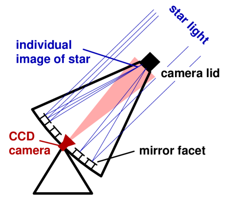
Figure 1: Mirror alignment technique: the telescope is pointed towards an appropriate star whereupon all mirror facets generate individual images of the alignment star in the focal plane. Actuator movements change the location of the corresponding light spot. This is observed by a CCD camera viewing the lid of the PMT camera which acts as a screen.

The basic algorithm is as follows [3, 4]: a CCD image of the camera lid is taken. Before alignment, and with all facet actuators positioned roughly at the center of their range, this image might appear as shown in Fig. 2. A facet which is to be aligned is moved in both axes. The effects on the image are recorded and provide all information required to move the corresponding spot to the center of the main focus. This procedure is repeated for all facets in sequence. The alignment accuracy is constrained by the CCD resolution, the actuator step size, and the mechanics of the facet supports, as well as by the design of the alignment algorithm.

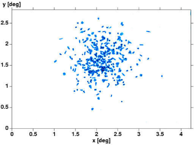
Figure 2: Image of a star on the camera lid before alignment, using a logarithmic intensity scale. The coordinates $x$, $y$ refer to the CCD image, translated into degrees using the known focal length of the CCD optics. The origin is at the lower left corner of the CCD chip. Each spot corresponds to a mirror facet. The spread of the spots reflects the precision in the alignment of the facet support brackets on the dish, about $0.5^{\circ}$, doubled due to reflection.

2.1 The monitoring CCD cameras

Given the large number of mirror facets on each H.E.S.S. telescope, a reliable and automatic scheme for mirror alignment is required. Such a scheme is implemented using the CCD camera to record the star images and to provide feedback for the actuator movements. The camera (“Lid CCD”) is located at the center of the dish and is used to view images of stars on the closed lid of the PMT camera. In addition, each H.E.S.S. telescope is equipped with a a second CCD camera (“Sky CCD”) which is mounted off-axis viewing the sky, and which serves as a guide telescope. The main parameters of these cameras and their optics are summarized in Table 1. The field of view of the lid CCD should be adjusted such that the central region of the PMT camera is covered and in addition at least three of eight positioning LEDs mounted at the corners of the PMT array are viewed . These LEDs serve to monitor deformations of the camera masts. The two CCD cameras are optimized differently. The lid CCD emphasizes a large dynamic range. During the alignment process, images generated by individual facets as well as the central spot with contributions from up to 380 facets must be resolved; the required frame rate is modest. The sky CCD, on the other hand, has a lower intensity resolution, but high frame rate in order to monitor telescope tracking continuously (during part of the measurements described here, the fast Ap1E was not yet available, and a slower ST7 camera was substituted). Both cameras are controlled using a PC running Linux, and the images produced may be directed into the main data stream (during normal operation), and/or to a specialized mirror alignment process. For the mirror alignment procedure only the lid CCD is used.

	Lid CCD	Sky CCD
Optics	Nikkor lens	Vixen 120 NA S refractor
	180 mm, f/2.8	800 mm, f/6.7
Camera type	Apogee Ap2Ep	Apogee Ap1E / Sbig ST7
Pixels	1536 x 1024	768 x 512
Pixel size	9.9”	2.3”
Field of view	$4.23^{\circ}$ x $2.82^{\circ}$	$0.51^{\circ}$ x $0.33^{\circ}$
Full-frame readout	45 s	0.3 s (Ap1E) / 12 s (ST7)
ADC	16 bit	14 bit / 16 bit (ST7)

Table 1: Characteristics of the two monitoring CCD cameras. During the initial work, an ST7 was used for the “Sky CCD”, replaced later by an Ap1E.

2.2 CCD image analysis

For the mirror alignment stars between -1.5 and 2.0^mag were used, with typical exposure times in the 0.2 to 16 s range; the measurement of the point spread function was performed in the -1.5 to 4.1^mag range, with exposures from 0.7 to 100 s. After alignment the image of a star typically contains a few $10^{6}$ electron charges, spread over O(100) CCD pixels. Signals are therefore very large compared to typical noise levels of 11 electrons (rms) per pixel. During the alignment, isolated images generated by individual mirror facets contain 2000 or more electrons.

CCD image processing relies on the eclipse library [5] from the European Southern Observatory (ESO), supplemented by additional methods. Details of the image processing differ between the mirror alignment procedure – where the emphasis is to define spot locations in a relatively short time – and the measurement of the point spread function – where the signal regions must be defined without discarding the tails of the intensity distribution.

In the mirror alignment procedure, light spots generated by individual mirror facets need to be identified. The detection of these spots is based on the difference of two CCD images taken in sequence for different positions of one of the alignment actuators of a certain mirror facet. The subtraction of the two images eliminates spots generated by other mirror facets, images of secondary stars, and inhomogeneous background illumination (such as moon light partially shadowed by the steel structure). Only the images generated by the mirror facet which was moved remain, and are usually easy to identify. Various consistency checks are applied during the analysis of the two CCD images. These include checks for intermediate tracking problems, changing weather conditions, and accidental identification of image artefacts. The difference method is very robust concerning image quality and therefore the preparation of the raw images can be rather simple. In a first step the (assumed constant) background level in the image (i.e., electronics offset, dark current, background light) is estimated by calculating the median of the pixel intensities, and is subtracted. The background subtracted images are cleaned by a 3x3 median filter in order to eliminate single hot pixels. A 3x3 Gaussian filter smoothes the images and simplifies the detection of image objects.

For the determination of the point spread function, the correct removal of the background and the identification of pixels belonging to the light spots are of prime concern. Faint tails of the intensity distribution need to be included without the introduction of a pedestal due to an underestimated background level. In a first step, the spot location is estimated using the image object detection algorithm of the eclipse library. The background level is then determined by applying a Gaussian fit to the distribution of pixel intensities using a relatively small area around the spot location. Because of the good homogeneity of the CCD chip, a flat-fielding correction can be omitted. To determine the pixels belonging to the star image, a special spot extraction algorithm has been developed. The area surrounding the spot is divided into segments for which the total intensities are calculated. Segments with negative total intensities are discarded. This is repeated for increasing segmentations of the remaining area. After the isolation of the signal region the center of gravity of all associated pixels is calculated. In case the newly determined spot location differs by more than a quarter of an image pixel from the previous location, the spot extraction is reiterated.

Extensive tests were performed to ensure that the procedures to define signal pixels do not introduce a bias in the determination of the point spread function and image shape. In addition, the results were verified using an independent analysis based on an alternative segmentation algorithm [6, 7, 8].

2.3 Location of focus

For optimal imaging, a Cherenkov telescope should be focused at the height of the shower maximum or somewhat higher [9]. For a typical distance to the shower maximum of $D\approx 8$ km, this implies that the focal plane should be positioned at $d\approx f/(1-f/D)\approx f+28\mbox{ mm}$, where $f$ is the nominal focal length. In case of the H.E.S.S. telescopes, the mirror alignment was carried out using the images of stars on the camera lid, positioned at $f=15.00$ m. The corresponding focus for shower images is then located about 30 mm behind the lid, and concident with the entrance of the array of Winston cones mounted in front of the PMTs. The Winston cones then act as non-imaging light concentrators, funnelling light onto the photocathodes. Therefore, after focusing star images on the camera lid, the PMT camera is at the optimal focus for shower images.

2.4 Alignment algorithm

The position of an individual light spot in the focal plane, $\mathbf{x}\equiv(x_{1},x_{2})$, is given by a function

$$\mathbf{x}=f(q_{1},\ldots,q_{6},\mathbf{a})\,,$$ (1)

which depends on the position and orientation of the corresponding facet support, $q_{i}$, and on the position of both actuators, $\mathbf{a}\equiv(a_{1},a_{2})$. Actuator positions are measured in units of counts of the Hall sensors, which monitor turns of the alignment motors (see Part I for a detailed description of the facet support units, and of the facet actuators and the associated control electronics). As the explicit expression for $f$ is rather complex and the exact values of the $q_{i}$ are hard to determine, a linear approximation is used to relate $\mathbf{\Delta x}$ and $\mathbf{\Delta a}$:

$$\mathbf{\Delta x}=\mathbf{T}\,\mathbf{\Delta a}\,,\quad\mathbf{\Delta a}=\mathbf{T^{-1}}\mathbf{\Delta x}$$ (2)

The transformation matrix

$$\mathbf{T}=\left(\begin{array}[]{cc}\delta x_{1}/\delta a_{1}&\delta x_{1}/\delta a_{2}\\ \delta x_{2}/\delta a_{1}&\delta x_{2}/\delta a_{2}\end{array}\right)$$ (3)

is determined by driving both actuators individually for a fixed number of counts while imaging the change in $\mathbf{x}$ with the lid CCD camera. The components of $\mathbf{T}$ are correlated due to the geometry of the facet support triangles, which are mounted on the dish with a fixed orientation:

$${\delta x_{1}/\delta a_{2}\choose\delta x_{2}/\delta a_{2}}\simeq\mathbf{R_{120}}{\delta x_{1}/\delta a_{1}\choose\delta x_{2}/\delta a_{1}}\,,\quad\mathbf{R_{120}}\equiv\left(\begin{array}[]{cc}-1/2&-\sqrt{3}/2\\ \sqrt{3}/2&-1/2\end{array}\right)$$ (4)

Here, $\mathbf{R_{120}}$ accounts for the angle of $\sim 120^{\circ}$ between the two directions of movement. The function $f$ is not strictly linear in $\mathbf{a}$ so the transformation matrix itself is a function of $\mathbf{a}$ and its components vary by some $\pm 10$ % for the whole range of the actuators. The validity of a certain matrix $\mathbf{T}$ is thus confined to a small range. To move a facet spot over a larger distance, an iterative procedure has to be used, with a compromise between precision and number of the iterations required (and hence the time required for alignment). Various procedures (“alignment algorithms”) have been studied. They differ, for example, in the effort made to determine $\mathbf{T}$ or in the step sizes.

To investigate the performance of different alignment algorithms, a simulation of the facet support mechanism and of the alignment process has been developed. (With the intention of concentrating on the inaccuracies caused by the finite step size of the actuators and by the uncertainty of the transformation matrix, the influence of the CCD imaging with its finite pixel size and noise was not simulated in detail.) For each algorithm investigated, $10^{5}$ mirror alignments have been simulated repeatedly for various distances of the mirror facet to the center of the dish. For reference, the alignment was first simulated using the exact representation of $\mathbf{x}$ (Eq. (1)) to determine the maximum achievable accuracy. In this case, the deviation from the nominal position is only due to the uncertainty of one count in each actuator position and represents the limits of the hardware. The simulation resulted in a distribution for individual light spots in the focal plane with a rms deviation of $0.015$ mrad and a worst case of $0.051$ mrad (see Fig. 3).

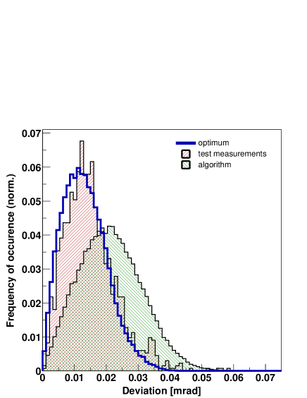
Figure 3: Alignment accuracy for individual light spots in the focal plane, determined in a laboratory test setup. The narrow filled histogram shows the experimental results, obtained by repeating the positioning cycle many times. The open histogram represents the theoretical optimum based on simulations. It is in good agreement with the results obtained from measurements with the test setup. The wider filled histogram represents the alignment accuracy of the algorithm chosen to align the telescopes, which represents a compromise between speed and precision. The deviations shown here refer to image coordinates, which are doubled due to reflection compared to the deviations in the orientation of facets.

This is in good agreement with test measurements of the facet support mechanics ($0.017$ mrad rms, see Fig. 3 and also Part I). After simulating the alignment accuracy for various algorithms, the algorithm described in the following section was chosen; its rms deviation of $0.023$ mrad is only marginally worse than the optimal case.

2.5 Alignment procedure

In addition to achieving a high alignment accuracy, the algorithm should enable the fast and reliable realignment of the mirror facets, in case the point spread function is observed to deteriorate over time. This is accomplished by splitting the procedure into two parts. During the initial alignment certain parameters are determined and stored in a database for further usage. These parameters include the range and position of the actuators and the final matrix to transform between CCD and actuator coordinates, valid near the center of the camera. The realignment procedure does not redetermine these values but simply retrieves them from the database. Since this transformation matrix depends primarily on the orientation of the facets, it should not vary with time, and in fact no significant changes were observed over several months. Following this approach, the time-consuming determination of these parameters has to be performed only once. The time required to align mirrors is to a significant extent determined by the CCD readout time. Another criterion was therefore to minimize the number of CCD exposures and wherever possible, only preselected CCD regions are read out.

The initial alignment procedure for a facet consists of several steps. At first the correct connection to the corresponding node on the branch cable is checked (see Part I). Next the range of both actuators is determined (refered to as “referencing”). As the actuator motors are not equipped with encoders and only provide information about the direction and amount of their travel, the lower stop is used as an internal position reference. The upstrokes of both actuators are determined by driving them to the lower stop and measuring the range from there to the upper stop. The valid range for positioning the actuators is then slightly reduced at both ends (by 5%) to avoid driving the actuators into the springs at the stops, reducing the potential of mechanical failure. Finally both actuators are driven to the lower end of their range to move the facet image out of the field of view of the lid CCD camera. Electrical problems and most types of mechanical defects will show up in these steps; the referencing is therefore also used to test the modules. These first two steps of the initial alignment procedure may take place during daytime; no optical feedback is required.

The aim of the next step is to identify the individual image of a star (spot) corresponding to the mirror facet to be aligned, and to determine a coarse transformation matrix for positioning the spot near the nominal position (“coarse alignment”). The nominal position is defined by the center of gravity of the facets which have been already aligned (the “main spot”). Due to the lack of a main spot for the first few facets, the spot of a laser pointer is used instead. The facets are aligned in sequence, with only one unaligned spot in the CCD field of view at a given time; images from other unaligned facets remain outside the field of view. A good starting point for positioning the spot of a facet inside the field of view is to move both actuators of a facet to the center of their range (Fig. 2 shows the resulting spread for all facets). Facets which have their image still outside of the CCD field of view ($\sim$2%) must be pre-aligned with human intervention. Next, a CCD image is taken. One of the actuators is then driven a predefined number of counts and another CCD image is taken. Here a 2$\,\times\,$2 CCD pixel binning is used which is sufficient for deriving a coarse transformation matrix, while significantly reducing exposure and CCD image readout times. From the analysis of these images, two elements of the transformation matrix are determined. Given these two elements, the other two can be estimated with sufficient precision on the basis of Eq. (4), due to the fixed geometry of the facet supports. Based on the measured spot location and the estimated matrix, both actuators are then driven to move the facet spot to the location of the main spot.

The initial alignment ends with the determination of the transformation matrix with maximum accuracy followed by the positioning of the facet spot at the center of the main spot (“fine alignment”). The procedure is similar to the coarse alignment; however, the transformation matrix is derived for both actuators individually and a 1$\,\times\,$1 CCD pixel binning is used. To obtain an accurate transformation matrix for the area around the main spot, the facet spot is placed at positions symmetrically surrounding the main spot. With this approach, the resulting transformation matrix is essentially perfect for the vicinity of the main spot. This step is illustrated in Fig. 4. The image readout time is reduced by retrieving only the relevant small sub-frame of the CCD image containing the spots.

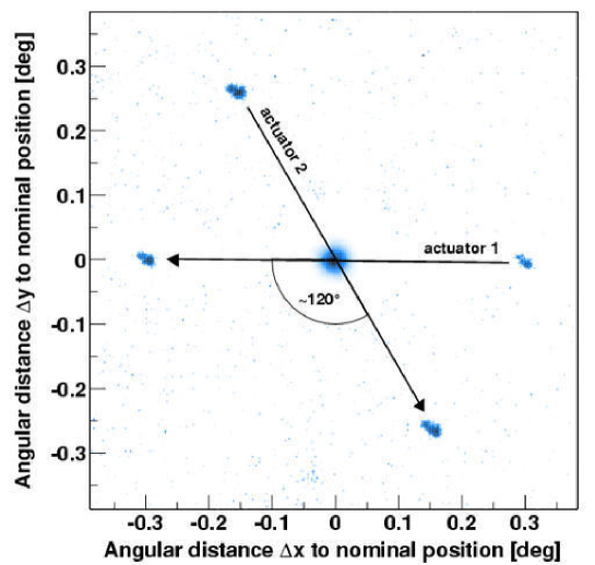
Figure 4: Superposition of four images taken by the lid CCD camera during the fine alignment, demonstrating the effect of the alignment actuators. In turn, each of the two actuators of a facet was moved a certain distance up and down, starting from a position in the central spot (which is scaled down for better visibility of the single spots). The resulting four displaced spots serve to calibrate the actuator movements. The angle of $\sim 120^{\circ}$ between the two directions is due to the geometry of the facet support triangle.

The realignment procedure is essentially a fine alignment of a single actuator without deriving a new transformation matrix. The spot of a given facet is moved out of the main spot, located, and driven back to the exact center of the main spot. This technique requires two CCD exposures to locate the facet spot, before and after the facet is moved. An even faster realignment was achieved by omitting the ‘before’ exposure and using the known transformation matrix to predict where to search for the spot generated by the facet, after it is moved out of the main spot. However, secondary stars accidentally overlapping the facet spot are then not corrected and may result in slight alignment errors.

We note here that mirrors are aligned relative to the main spot (or a laser spot for the first few mirrors). This procedure can be applied even if the telescope does not track the star perfectly. In any case, with a measured absolute pointing precision of about one arc-minute and relative tracking deviations with respect to the average orbit of a few arc-seconds, tracking of the H.E.S.S. telescopes is perfect for all practical purposes. This holds in particular for the measurements of the point spread function discussed later; using bright stars, stable tracking over a few seconds of exposure time is sufficient.

Table 2 summarizes the net duration for the different steps of the alignment procedure.

step	approximate net duration per
	facet	telescope
connection	1 sec (daytime)
referencing	8 min (daytime)	51 hrs
coarse alignment	90 – 120 sec
fine alignment	90 – 150 sec	24 hrs
total	12 min	75 hrs
realignment	45 – 75 sec	6.5 hrs
fast realignment	25 – 40 sec	3.5 hrs

Table 2: Duration of the alignment procedure. The first two steps can be performed during daytime while the two alignment steps require darkness but allow for the moon to be partially visible. The duration of the steps where optical feedback is required varies with the brightness of the star used for alignment. Under normal circumstances, the initial alignment needs about two weeks and the realignment can be performed in one to two nights.

The steps requiring optical feedback can be performed during times where the moon is partially visible, and do not interfere with the schedule for taking very high energy gamma-ray data.

3 Point spread function

All mirror facets of the first H.E.S.S. telescope (for historical reasons labelled “CT03”) were successfully aligned in January/February 2002; the second telescope (“CT02”) was aligned in November/December 2002. In construction, all four H.E.S.S. telescopes are identical, and should therefore exhibit identical mechanical and optical characteristics . During the initial alignment of the telescopes, the PMT cameras were not yet available; instead, dummies of roughly the same weight and with front surfaces in the same location as the real camera lid were installed.

To study the point spread function after the alignment of the telescopes was completed, a variety of stars were used, covering a wide range of locations within the field of view (Fig. 5 left) and of elevation and azimuth angles for the telescope pointing (Fig. 5 right). Because of the limited field of view of the lid CCD camera of the first telescope, the entire field of view of the PMT camera – with $5^{\circ}$ diameter – could not be covered in these measurements. For the second telescope, the camera was pointed slightly off-axis, to cover both the center of the field of view, and – in one direction – the edge.

The measured point spread functions of both telescopes are essentially identical.

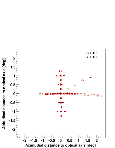
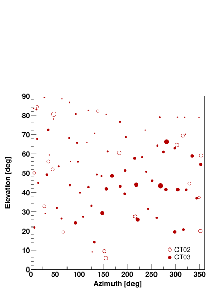
Figure 5: Left: Locations in the field of view where the point spread function was measured. The origin refers to the optical axis of the telescope. Full symbols: first telescope (CT03), open symbols: second telescope (CT02). Right: Elevation/azimuth values of telescope pointing where the point spread function was measured. The azimuth coordinate increases from north to east. The size of the points indicates the brightness of stars.

Fig. 6 shows a typical result, namely the CCD image of the image of a star on the camera lid, in relation to the size of a hexagonal PMT pixel. The image spot is symmetrical, without pronounced substructure, and the width of the spot is well below the PMT pixel size. As mentioned earlier, the signal charges in the CCD pixels are very high, so that noise and statistical fluctuations in the signal are of no concern.

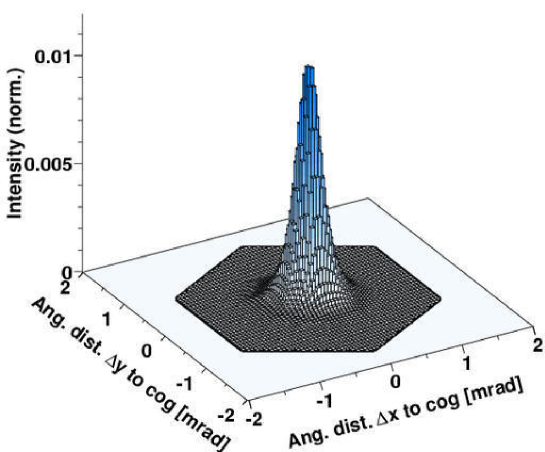
Figure 6: Image of a star on the camera lid of CT03, as viewed by the lid CCD camera. The boxes correspond to CCD pixels, and the hexagonal border indicates the size of a pixel of the PMT Cherenkov camera. The image was taken at an elevation of $70^{\circ}$, near the alignment range.

To quantify the width of the intensity distributions, different quantities are used. These include the rms width $\sigma_{proj}$ of the projected (1-dimensional) distributions, the rms width $\sigma$ of the two-dimensional distribution, and the radii $r_{60}$ or $r_{80}$ of circles around the center of gravity of the image, containing 60% or 80% of the total intensity, respectively. For a symmetrical Gaussian intensity distribution, the following relations hold:

$$\sigma = \sqrt{2}\sigma_{proj}$$ (5)

$$r_{60} = \sqrt{2\ln{(5/2})}~{}\sigma_{proj}=\sqrt{\ln{(5/2)}}~{}\sigma$$ (6)

$$r_{80} = \sqrt{2\ln{5}}~{}\sigma_{proj}=\sqrt{\ln{5}}~{}\sigma$$ (7)

On the optical axis, the point spread function is characterized by values $\sigma=0.33$ mrad (CT02) and 0.32 mrad (CT03) (compared to an initial specification of 0.71 mrad), $\sigma_{proj}=0.23$ mrad and 0.23 mrad (compared to 0.50 mrad), $r_{60}=0.30$ mrad and 0.28 mrad (compared to 0.68 mrad) and $r_{80}=0.41$ mrad and 0.40 mrad (compared to 0.90 mrad).

3.1 Variation across the field of view

Optical aberrations are significant in Cherenkov telescopes, due to their single-mirror design without corrective elements and their modest $f/d$ ratios. At some distance from the optical axis, one therefore expects the width $\sigma$ of the point spread function to grow linearly with the angle $\theta$ to the optical axis. On the axis, the width of images is determined by the intrinsic optical quality of the mirror facets, $\sigma_{o}$, by the aberrations caused by the fact that most facets are inclined relative to the optical axis, $\sigma_{a}$, and by the precision $\Delta_{align}$ with which the individual mirror facets are aligned. To a good approximation, the width of the point spread function should hence be given by

$$\sigma=(\sigma_{o}^{2}+\sigma_{a}^{2}+4\Delta_{align}^{2}+c\theta^{2})^{1/2}$$

where the factor 4 accounts for the doubling of facet alignment errors due to reflection. The constant $c$ describes the aberrations for off-axis rays and is proportional to the inverse square of the $f/d$ ratio of the telescope.

With increasing inclination to the optical axis the spot is indeed observed to widen (Fig. 7); it also develops an asymmetric tail away from the optical axis. A more quantitative description of the spot shape is provided by projections of the intensity distribution on the radial and tangential directions, shown in Fig. 8 for angles of $0^{\circ}$, $0.96^{\circ}$ and $2.05^{\circ}$ relative to the optical axis.

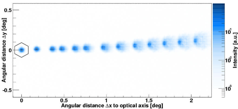
Figure 7: Star images viewed on the camera lid of CT02, for different distances from the optical axis. For comparison, the pixel size is indicated.

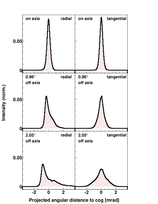
Figure 8: Intensity distributions for images of stars on the camera lid of CT02, for stars on the optical axis (top row), $0.96^{\circ}$ off-axis (middle row) and $2.05^{\circ}$ off-axis (bottom row), projected onto the radial direction (left) and onto the tangential direction (right).

For measurements near the elevation angle where the telescope was aligned, around $65^{\circ}$, Fig. 9 summarizes the spot parameters as a function of the angle $\theta$ to the optical axis. In addition to $r_{80}$, the rms widths of the distributions projected on the radial ($\sigma_{radial}$) and tangential ($\sigma_{tangential}$) directions are given. The radial axis goes from camera center to the center of the spot, the tangential axis is the corresponding orthogonal direction. The measurements demonstrate that the spot width depends primarily on $\theta$; any other variation, depending on the exact location in the field of view, is small and no other systematic trend is found. With increasing angle to the optical axis, the spot width increases, following a shallow parabola at small angles. Later a transition to a linear dependence is observed, as expected on the basis of the modeling of the optical system (see Part I). The images become slightly elliptical, elongated in the radial direction, again as expected. The two telescopes show very similar point spread functions; the last three points for $r_{80}$ of CT03 in Fig. 9 are marginally above the corresponding values for CT02, but are still consistent given the typical scatter of the measurements, and taking into account the varying observing conditions, night sky brightness etc.

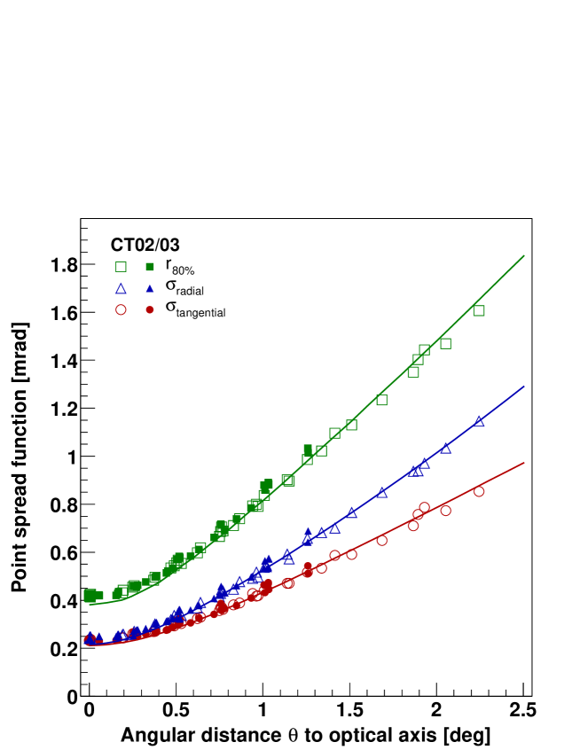
Figure 9: Width of the point spread function as a function of the angular distance $\theta$ to the optical axis, at elevations around $65^{\circ}$. Different measures of the width of the point spread function are shown: the rms width in the radial direction (triangles), the rms width in the tangential direction (circles) and the radius of a circle enclosing 80% of the light, centered on the center of gravity of the image (squares). Off-axis data were taken at different points of the field of view, see Fig. 5. Full symbols: first telescope (CT03), open symbols: second telescope (CT02). For CT03, the CCD camera used to view the spot was aligned to provide a symmetric field of view with respect to the optical axis, limiting its field of view to $1.5^{\circ}$. The CCD camera of CT02 has an asymmetric field of view and provides measurements out to $2.3^{\circ}$. The lines indicate the result of simulations, using the known point spread functions of the mirror facets as input, combined with the precision of the alignment algorithm as derived from the simulations of the alignment process.

To verify that the measured intensity distribution is quantitatively understood, Monte Carlo simulations of the actual optical system were performed, including the exact locations of all facets, shadowing by camera masts, etc. As further input, the measured average spot size of the mirror facets and the precision of the alignment algorithm were used. The latter is govered primarily by the accuracy with which images of individual facets can be located in the CCD images, which enters both directly and indirectly via errors in the determination of the transformation matrix and which results in an overall alignment uncertainty of 0.10 mrad for the individual spots. The errors in the location of images were derived by moving some individual mirrors in steps along straight lines and comparing expected and measured positions, and by comparing the positions determined with different algorithms for image analysis.

The results are included in Fig. 9 as solid lines, and are in good agreement with the measurements. The simulations tend to slightly underestimate the point spread function on axis. A likely explanation is that the simulations use identical Gaussian point spread functions for the individual facets, whereas some of the actual measured spots are highly non-Gaussian, and in extreme cases even exhibit double sub-spots.

3.2 Variation with telescope pointing

Given the weight of the facets and the size of the dish, it would be non-trivial and quite costly to design a dish structure which does not deform under the influence of gravity when moved in elevation. The structure of the H.E.S.S. telescopes represents a compromise between stiffness versus weight and cost. Over the working range in elevation, about $30^{\circ}$ to $90^{\circ}$, the influence of gravity-induced deformations should be small compared to the intrinsic point spread function of the mirror facets, specified by the requirement that 80% of the light is contained in a circle of 1 mrad diameter.

To test for variations of the spot size with telescope pointing, the (most sensitive) on-axis point spread function was measured over a wide range of pointings, see Fig. 5. No significant dependence of the point spread function on telescope azimuth was detected at fixed elevation. This is non-trivial, since in the H.E.S.S. telescopes additional stiffness is provided by tensioning the dish between the two elevation towers. A deviation from perfect flatness of the azimuthal rail could introduce an azimuth-dependent modulation of the tension and hence of the shape of the dish.

What is both predicted (see Part I) and observed is a variation of the point spread function with elevation, presumably mainly due to deformations of the dish structure, but also with small contributions from the facet support units. Fig. 10 illustrates how the measured spot width changes with elevation. The width is at a minimum around $65^{\circ}$ to $70^{\circ}$, the angle at which the facets were aligned. For the range of elevation angles most relevant for Cherenkov observations (above $45^{\circ}$) the spot size $r_{80}$ varies by less than 10%; at $30^{\circ}$ it is about 40% larger than the minimum size. At the alignment elevation the on-axis spot is essentially circular; at lower and higher elevations the spot becomes elliptical and is narrower in the elevation direction as compared to the orthogonal direction, along the telescope azimuth. At low elevations, the deviation between the spot widths along its two main axes can reach 50%.

To provide a description for use in simulations etc., the spot size as a function of elevation $\Theta$ was parametrized by the function

$$r_{80}(\Theta)=(r_{eff}^{2}+d^{2}(\sin\Theta-\sin\Theta_{0})^{2})^{1/2}$$

with $r_{eff}=0.41$ mrad, $d=0.96$ mrad and $\Theta_{0}=66^{\circ}$. The parameter $d$ refers to the deformation of the dish relative to the alignment position; the measured value agrees within 25% with the value expected on the basis of finite element simulations of the dish. A more detailed discussion of the dish deformations will be given in section 4.

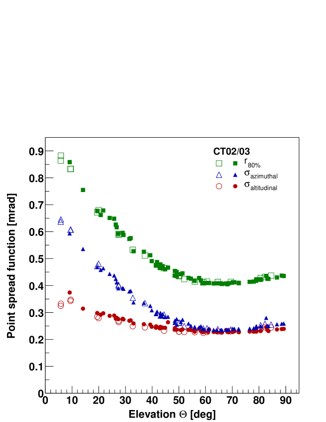
Figure 10: Width of the point spread function as a function of elevation $\Theta$. Full symbols: first telescope (CT03), open symbols: second telescope (CT02).

3.3 Long-term stability of the point spread function

While a realignment of facets is possible within a relatively short time, the telescope structure was designed for good long-term stability, to minimize drifts in the imaging characteristics.

The point spread function of the first telescope (CT03) has been measured several times over the course of nearly a year, first in February 2002 after the initial alignment, then in Summer 2002 after the PMT camera was mounted, and again in December 2002 when the mirror of the second telescope (CT02) was aligned, and in July 2003. An increase in the width of the (on-axis) point spread functions of up to 15% was observed between the first and the second measurement, in particular in $r_{80}$ and in the horizontal direction of the image. This change is very likely caused by the difference of about 100 kg between the actual camera and the dummy load used during the initial alignment; the forces generated by the camera arms represent a significant contribution to the gravity-induced deformations of the dish. Since the point spread function after installation of the camera was still well below specifications, a realignment was not required. Between the second, third and forth measurement, the point spread function was stable.

4 Study of deformations of the dish structure

The remote control of individual facets offers additional options to study the mechanical characteristics of the dish. Once facets are aligned – i.e., the actuators are referenced relative to an absolute system and the transformation between actuator coordinates and image coordinates is determined – spots generated by individual facets can be arranged in arbitrary patterns. As an example, Fig. 11 shows the spots corresponding to individual mirror facets arranged in the form of a square matrix. Each element of the matrix is the image of the observed star generated by one facet. One notices significant differences between facets; some of the images are notably elongated, while others are approximately circular spots. Part of these differences are caused by variations in the quality of the mirror facets; the bulk of the effect, however, are optical aberrations for off-axis facets. Facets at the edge of the dish generate the majority of the elongated images, and the orientations of the images correlate with the position on the dish.

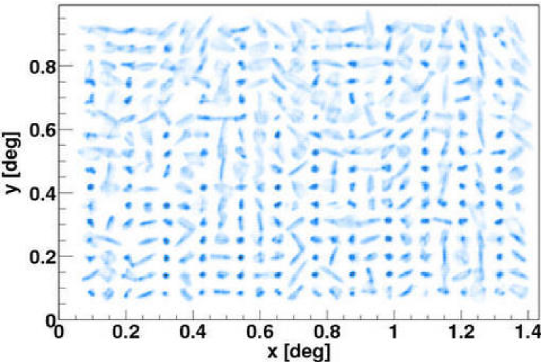
Figure 11: Individual spots arranged in the form of a matrix. Each spot corresponds to the image of the observed star generated by an individual mirror facet; rather than combining all individual spots at the center, the actuators were driven to generate this specific pattern.

The matrix pattern enables one to study deformations of the dish structure in much greater detail, than is possible by observing only the effect on the overall point spread function. For this purpose, images of the matrix were taken for different elevations of the dish. By tracking the relative movement of individual spots with elevation, the deformation of the corresponding locations in the dish can be determined. Fig. 12 shows the deflection of facets between $65^{\circ}$ and $29^{\circ}$ elevation. Deformations are particularly strong in the regions where the dish is supported and where the camera arms are attached.

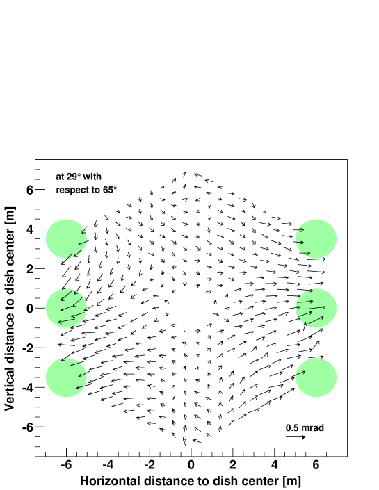
Figure 12: Change in the orientation of facets with elevation between $65^{\circ}$ and $29^{\circ}$ elevation. The deflection of a given facet is indicated as an arrow drawn at the position of the facet on the dish; the length of the arrow is proportional to the square root of the angular distance a facet is deflected. Shaded areas indicate the regions where camera arms are attached (top and bottom areas) and where the dish is supported (middle).

The data on facet deflection allows a direct comparison between the finite element (FEM) simulations and the actual performance of the dish. In the design of the dish, FEM simulations were carried out for elevations of $20^{\circ}$, $50^{\circ}$ and $90^{\circ}$ (see Part I). In the simulations, the middle elevation was defined as the reference point were the facets are aligned . To directly compare data and FEM simulations, facet deflections were determined relative to the facet pointing at $50^{\circ}$ elevation. The rms deflection for all facets is shown in Fig. 13, as a function of elevation, separately for the horizontal and vertical deflections.

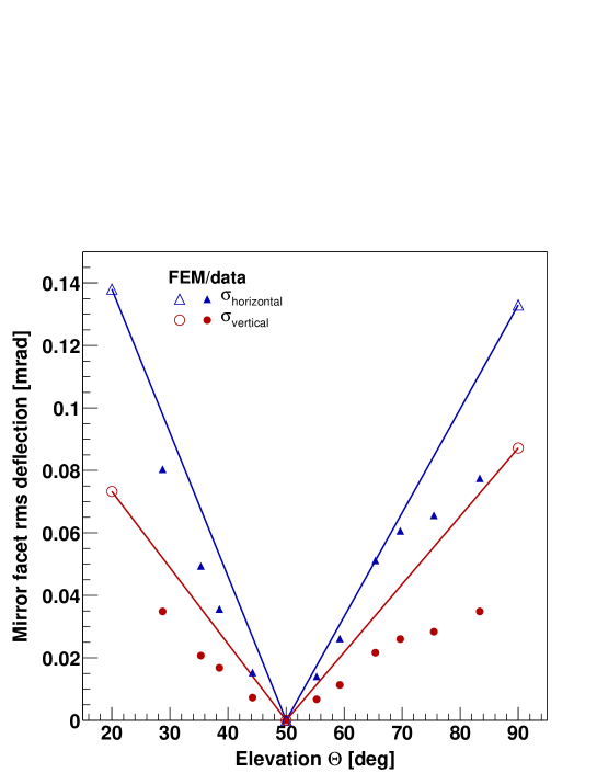
Figure 13: Rms horizontal and vertical deflection of mirror facets relative to $50^{\circ}$ elevation, for data (closed symbols) and for the FEM model of the dish (open symbols). Model calculations are only available for $20^{\circ}$, $50^{\circ}$ and $90^{\circ}$; the straight lines drawn between the model points should however represent a reasonably reliable interpolation. The data were obtained for CT03.

Data and simulation agree reasonably well; the dish actually deforms less than predicted. Given the differences between the actual dish and the simplified model assumed in the simulations, such differences are to be expected – for some beams, slightly modified wall thicknesses were used, weight was added due to material in the nodes of the structure, walkways etc. Also, the FEM model made very conservative assumptions concerning the stiffness of the nodes of the spaceframe backing the dish.

In summary, we conclude that the FEM simulations have proven a reliable (or even conservative) tool for the design of the H.E.S.S. instruments.

5 Absolute pointing of the telescope

The discussion was so far mainly concerned with the point spread function, i.e. the width of the image. A second important quality criterion of a Cherenkov telescope is the pointing precision. For strong gamma-ray sources, the location of the source on the sky can be determined with a statistical precision of a few arc-seconds. Systematic errors – resulting, for example, from deviations of the telescope pointing – should be reduced to a similar level. This is non-trivial, since image information obtained during normal operation – such as stars in the field of view – cannot be used to monitor telescope pointing with sufficient precision, given the coarse pixel size. Cherenkov telescopes therefore have to rely primarily on shaft-encoder data for pointing (in the case of the H.E.S.S. telescopes, this information is augmented by images from the optical guide telescope – the “sky CCD”), and one needs to apply corrections for effects such as the bending of the camera arms.

A detailed discussion of this issue is beyond the scope of this paper and will be addressed elsewhere. Here, we will only summarize the main conclusions obtained at this time:

• Deformations of the camera arms, which result in a shift of images relative to the PMT pixel matrix, are monitored by viewing the set of LEDs at the edge of the PMT camera using the lid CCD; the measured bending of the arms – expressed in terms of the image shift – is well described by $b=82.7"\cos{\Theta}$ .

• Using a parameterization to relate measured shaft encoder values to true pointing, a pointing precision of about 8” rms is obtained. The corrections account for the bending of the masts, but also for nonlinearities of the encoders, alignment errors of the telescopes azimuth and elevation axes, etc.

• Using in addition the information from the sky CCD camera when a star is in its field of view, pointing can be improved to less than 3” rms.

6 Summary

Using the first two telescopes of the H.E.S.S. system, an automatic alignment technique for the mirror facets has been developed and tested, and the optical properties of the telescopes were studied in detail.

The alignment of the 380 facets proceeded to a large extent automatically. Operator intervention was required only for a small fraction of facets where the actuator mechanics had problems and needed to be exchanged, or where the initial spot was not within the field of view of the CCD camera. In total, about 75 h are required in total to align all mirrors, about 2/3 of the work being possible during daytime. A realignment is possible within one or two nights.

The point spread function of a telescope depends on the optical design, on the quality of the individual mirror facets, on the precision of the alignment and on the mechanical stability of the dish and the facet supports. The quality of the mirror facets and the precision of the alignment system exceed specifications by a significant margin. At the time of the design, 0.5 mrad was specified for the rms width of the one-dimensional projection of the spot, evaluated on the optical axis where the spot size is minimal (see Part I). This value should be compared to the measured width of 0.23 mrad.

The point spread function is expected to broaden with increasing distance from the optical axis, and to vary slightly with elevation beause of gravity-induced deformations of the dish. The point spread function, measured around $65^{\circ}$ elevation and characterized by the radius $r_{80}$ of a circle containing 80% of the light, and is well described by

$$r_{80}=(0.42^{2}+(0.71\theta)^{2})^{1/2}~{}~{}~{}\mbox{[mrad]}$$

where $\theta$ is the angle to the optical axis in degrees. The point spread functions are almost identical for the two telescopes. Individual fits show a difference of 0.01 between the telescopes for the first coefficient, and of 0.05 for the second. Monte Carlo simulations using the measured facet characteristics as input predict

$$r_{80}=(0.38^{2}+(0.72\theta)^{2})^{1/2}~{}~{}~{}\mbox{[mrad]}$$

indicating that the telescopes behave as expected. With elevation $\Theta$, the on-axis spot size varies roughly as

$$r_{80}=(0.41^{2}+0.96^{2}(\sin\Theta-\sin 66^{\circ})^{2})^{1/2}~{}~{}~{}\mbox{[mrad]}$$

where $\Theta$ is given in degrees. This spot size should be compared with the PMT pixel size of 2.8 mrad.

References

- [1] W. Hofmann, Proc. of the 27th Int. Cosmic Ray Conf., Hamburg, 2001, M. Simon, E. Lorenz, M. Pohl (Eds.), p. 2785
- [2] K. Bernlöhr et al., submitted for publication
- [3] R. Cornils, I. Jung, Proc. of the 27th Int. Cosmic Ray Conf., Hamburg, 2001, M. Simon, E. Lorenz, M. Pohl (Eds.), p. 2879
- [4] W. Hofmann, H.E.S.S. Internal Note 98/15, 1998 (unpublished)
- [5] N. Devillard, “The eclipse software”, The messenger No 87 - March 19; see also http://www.eso.org/projects/aot/eclipse/
- [6] B. Jähne, Digitale Bildverarbeitung, Springer Berlin, Heidelberg, New York, 1993
- [7] J.P. Burt, T.H. Hong, A. Rosenfeld, IEEE Trans. on Systems, Man and Cybernetics 11 (1981) 802
- [8] S. Gillessen, Diploma Thesis, Heidelberg 1999
- [9] W. Hofmann, J. Phys. G 27 (2001) 933