Cosmological Evolution of the Hard X-ray AGN Luminosity Function and the Origin of the Hard X-ray Background

Abstract

We investigate the cosmological evolution of the hard X-ray luminosity function (HXLF) of Active Galactic Nuclei (AGNs) in the 2–10 keV luminosity range of $10^{41.5}-10^{46.5}$ erg s^-1 as a function of redshift up to 3. From a combination of surveys conducted at photon energies above 2 keV with HEAO1, ASCA, and Chandra, we construct a highly complete ($>$96%) sample consisting of 247 AGNs over the wide flux range of $10^{-10}-3.8\times 10^{-15}$ erg cm^-2 s^-1 (2–10 keV). For our purpose, we develop an extensive method of calculating the intrinsic (before-absorption) HXLF and the absorption ($N_{\rm H}$) function. This utilizes the maximum likelihood method fully correcting for observational biases with consideration of the X-ray spectrum of each source. We find that (i) the fraction of X-ray absorbed AGNs decreases with the intrinsic luminosity and (ii) the evolution of the HXLF of all AGNs (including both type-I and type-II AGNs) is best described with a luminosity dependent density evolution (LDDE) where the cutoff redshift increases with the luminosity. Our results directly constrain the evolution of AGNs that produce a major part of the hard X-ray background, thus solving its origin quantitatively. A combination of the HXLF and the $N_{\rm H}$ function enables us to construct a purely “observation based” population synthesis model. We present basic consequences of this model, and discuss the contribution of Compton-thick AGNs to the rest of the hard X-ray background.

1 Introduction

Revealing the cosmological evolution of the AGN luminosity function, which is directly linked to the accretion history of the universe and hence the formation history of supermassive black holes in galaxies, has been a main goal of X-ray surveys. Previously, most of these studies (e.g., Maccacaro et al., 1991; Boyle et al., 1993; Jones et al., 1997; Page et al., 1997; Miyaji, Hasinger, & Schmidt, 2000a) were made in the soft X-ray band ($\;\buildrel<\over{\sim}\;$3 keV) which could be subject to biases against absorbed AGNs. Hard X-ray surveys (above 2 keV) are a key ingredient to trace the luminosity function of the whole AGN population including obscured (type-II) AGNs, main contributors to the cosmic X-ray background (CXB or XRB; for reviews see e.g., Boldt 1987 and Fabian & Barcons 1992).

Earlier work on the hard X-ray luminosity function (HXLF) by Boyle et al. (1998) and La Franca et al. (2002) indicates strong evolution of the HXLF, like that seen in soft X-rays. Cowie et al. (2003) has constrained the 2–8 keV HXLF at two redshift bins ($z$=0.1–1 and $z$=2–4) mainly from Chandra surveys. They argued that the AGN number density for luminosities lower than $\approx 10^{44}$ erg s^-1 seems to peak at a closer redshift than those of higher luminosity, unless they assumed a very extreme redshift distribution for unidentified sources. This is consistent with the soft X-ray luminosity function (SXLF) result from a combined analysis of ROSAT and Chandra data (Hasinger, 2003). However, the X-ray samples used in the above studies of the HXLF are still limited in completeness and size. A further study using a much larger, highly complete sample over a wide luminosity-redshift range is necessary to unambiguously constrain the evolution of the luminosity functions of both type-I and type-II AGNs.

Recently Akiyama et al. (2003; hereafter A03) have completed an optical identification program of a 2–10 keV selected sample in the ASCA Medium Sensitivity Survey (AMSS; Ueda et al. 2001) from an area of 69 degree² in the northern sky (Dec. $>-10^{\circ}$) with a flux limit of $3\times 10^{-13}$ erg cm^-2 s^-1 (AMSSn sample). The AMSSn sample contains 85 identified AGNs, which is currently the largest hard-band selected AGN sample that covers the flux range above $\sim 10^{-13}$ erg cm^-2 s^-1 (2–10 keV). In this paper we also utilize another sample from an extension of the identification program of the AMSS in the southern sky. In total we now have 141 hard X-ray selected AGNs solely from ASCA surveys with completeness of 97% including the AMSS, the ASCA Large Sky Survey (=ALSS; Ueda et al. 1999a; Akiyama et al. 2000), the deep ASCA surveys in the Lockman Hole (Ishisaki et al., 2001), and in the Lynx field (Ohta et al., 2003). These highly complete ASCA samples provide an ideal opportunity to constrain the nature of the AGNs, in particular, at the intermediate redshift universe below $z\approx 1$. Furthermore, combining brighter AGN samples from HEAO1 surveys and fainter ones from Chandra surveys enables us to trace the cosmological evolution of AGNs in the 2–10 keV luminosity range of $10^{41.5}-10^{46.5}$ erg s^-1 at redshifts up to 3.

In this paper we directly constrain the evolution of AGNs that constitute a major part of the 2–10 keV X-ray background. We construct a hard X-ray (2–10, 2–8, or 2–7 keV) selected sample with an extremely high degree of completeness from HEAO1, ASCA, and Chandra surveys. The sample consists of 247 sources in total. In the analysis we fully consider the detector response and the X-ray spectrum of each source making use of the best information available. This step is crucial to correct for selection biases caused by using a count-rate (not flux) limited sample. We firstly formulate the absorption distribution function of AGNs and discuss its luminosity and redshift dependence. Then, we present our results of an intrinsic (before absorption) HXLF. Finally, we discuss the contribution of AGNs to the CXB by constructing a purely “observation based” population synthesis model. We adopt the cosmological parameters of ($H_{0}$, $\Omega_{\rm m}$, $\Omega_{\lambda}$) = (70$h_{70}$ km s^-1 Mpc^-1, 0.3, 0.7) as a default, but in some cases we also show results with ($H_{0}$, $\Omega_{\rm m}$, $\Omega_{\lambda}$) = (50$h_{50}$, 1.0, 0.0) for comparison with previous works. Throughout the paper the “Log” symbol represents the base-10 logarithm, while “ln” the natural logarithm.

2 Sample

To cover a wider luminosity and redshift range for studying the AGN HXLF, we construct a flux-limited sample by adding published data from the HEAO1 survey and Chandra Deep Field North (CDFN) survey to the ASCA sources. The whole sample contains 247 hard band selected AGNs (excluding BL Lac objects). The number of the sources and flux limit (2–10 keV) in each survey is listed in Table 1. The following subsections describe the details of each survey and selection criteria of the sample.

2.1 The HEAO1 sample

A flux-limited, hard X-ray selected sample from the HEAO1 surveys is included in our analysis as the brightest flux end sample. We use the same sample as used for follow-up spectroscopic studies with ASCA and XMM-Newton by Miyaji et al. (2003b). This enables us to take into account the best spectral information at present. It consists of 49 sources, (Part I) 28 AGNs from the HEAO1 A2 complete sample by Piccinotti et al. (1982) and (Part II) 21 AGNs from a region-limited subsample of the MC-LASS (HEAO1 A1/A3) catalog by Grossan (1992). Since our purpose is to constrain the global spectral distribution of AGNs, detailed modeling of individual sources is not crucial for our studies. Basically we refer to results of a single power law fit with a neutral absorber at the source redshift over the Galactic absorption, which are in most cases acceptable. One source (Kaz 102 / V1803+676) shows a very flat spectrum, which may be caused by an extreme warm absorber (Miyaji et al., 2003a). We treat the spectrum of this object as an unabsorbed power law with a photon index, $\Gamma$, of 0.96. In a few sources there is evidence for a strong warm absorber, dual absorbers and/or a soft excess (Miyaji et al., 2003b), where significant residuals are seen from an absorbed power-law model. For simplicity and consistency with analysis of the other samples, we only assume a single, neutral absorption even if the fit is not acceptable. Hence, the column density we use is an “effective” one that may partially contain the effects of warm or dual absorbers. A soft excess component, if any, is neglected in calculating the luminosity.

In the Part I sample we selected 28 emission-line AGNs from Piccinotti et al. (1982) brighter than 1.25 $R15$ c s^-1 in the first scan of the HEAO1 all sky survey at Galactic latitude of $|b|>20^{\circ}$. For convenience two Piccinotti AGNs (NGC 4151 and NGC 5548) located in the overlapping region of the Part II sample are included in the latter sample. We refer to the new identification of the HEAO1 source H 0917-074 as the Seyfert 2 galaxy MCG–1–24–12 ($z=0.0198$) revealed by Malizia et al. (2002). The $R15$ count rate is defined as a sum of the two detectors, HED and MED, from the HEAO1 A2 experiment (Marshall et al., 1980). The 1.25 $R15$ c s^-1 count rate corresponds to a flux limit of $2.7\times 10^{-11}$ erg cm^-2 s^-1 (2–10 keV) for a power law with $\Gamma=1.7$. The sample is 100% complete. Except for Mrk 590 and H 0917-074, which are observed by XMM-Newton (Miyaji et al., 2003b) and BeppoSAX (Malizia et al., 2002) respectively, the AGNs have been observed with ASCA.

The Part II sample comes from a complete flux-limited AGN sample constructed from the MC-LASS catalog. The area covers a 55 degree region from the North Ecliptic Pole. The count rate limit is 0.0036 LASS c s^-1, corresponding to $1.9\times 10^{-11}$ erg cm^-2 s^-1 (2–10 keV) for $\Gamma=1.7$. We exclude 3C 351 and H 1443+421 from the original Grossan (1992) catalog because of possible source confusion and/or misidentification problem. The completeness of the total Grossan sample is 86% (or 85% within our limited region according to comparison between the HEAO1 A1 and A3 catalogs). Grossan (1992) argues, however, that a majority of unidentified sources turned out to be active coronae (Galactic stars) or BL-Lac objects from a comparison with Einstein and ROSAT data. Thus, we make the first working hypothesis that the identification of the HEAO1 Part II sample is complete for AGNs other than BL Lac objects, and do not apply any completeness correction. Note that our results for the HXLF presented below are not affected over the statistical error by whether the completeness correction (85%) is applied to this sample or not. We have spectral data of ASCA or XMM-Newton for all the sources except H 1537+339, for which we assume a power law with $\Gamma=1.7$ and no absorption. For NGC 4151, whose X-ray spectrum is known to be highly variable and complex, we adopt $\Gamma=1.5$ and $N_{\rm H}$= $2\times 10^{23}$ cm^-2 as typical values from the results of Weaver et al. (1994). To convert the LASS count rate into physical flux unit in our analysis, we create an approximated energy response by scanning the quantum efficiency curve of the A1 detector given by Wood et al. (1984).

2.2 The ASCA sample

2.2.1 The AMSS

The AMSSn sample consists of 87 serendipitous sources in the AMSS X-ray catalog (Ueda et al., 2001) in the northern sky (DEC$>20^{\circ}$), detected with a detection significance larger than 5.5 $\sigma$ at a flux limit of $3\times 10^{-13}$ in the 2–10 keV band. The criteria for the detection significance and flux limit were set relatively conservative to lessen systematic errors due to the Eddington bias and source confusion. Detailed description of the optical identification is given in A03. They are identified with 78 AGNs, (including 3 BL Lac objects), 7 clusters of galaxies, and 1 galactic star. One source (1AXG J133937+2730) is still unidentified. The AMSS catalog was constructed only from “faint” fields with a total GIS count rate smaller than 0.8 c s^-1. As mentioned in Ueda et al. (1999b), this could cause a bias against bright sources with fluxes larger than $\sim 10^{-11}$ erg cm^-2 s^-1 (2–10 keV). Hence, to ensure the completeness we also apply an upper limit of $5\times 10^{-12}$ erg cm^-2 s^-1 (2–10 keV) to define a good statistical sample for the present study. Finally, we have 74 identified AGNs from A03 after excluding the BL Lac objects and the brightest source 1AXG J122135+7518. The survey area is calculated as a function of limiting count rate by the same technique as described in Ueda et al. (1999b). The total area covered for the AMSSn sample is 69 deg² at bright fluxes. Except for 1AXG J233200+1945 and 1AXG J234725+0053, for which XMM-Newton follow-up observations have been performed, we only have information of the hardness ratio $HR1$, defined as $(C1-C2)/(C1+C2)$, where $C1$ and $C2$ represent the 2–10 keV and 0.7–2 keV vignetting-corrected count rate, respectively.

Furthermore, we are conducting an extension of the identification program of the AMSS sources to the southern sky (we here tentatively call it the “AMSSs sample”; Akiyama et al., in preparation), including X-ray sources in a new Gas Imaging Spectrometer (=GIS; Ohashi et al. 1996) source catalog constructed from ASCA archival data taken after 1997 (Ueda et al., in preparation). The extended sample currently available provides 20 additional identified AGNs to the AMSSn sample with 2 unidentified objects.

2.2.2 The ALSS

The ASCA Large Sky Survey (ALSS) is a wide-area unbiased source survey covering continuous area of 5.5 deg² near the North Elliptic Pole (Ueda et al., 1998, 1999a). From 34 sources detected in the 2–7 keV band with the Solid-state Imaging Spectrometer (=SIS; Burke et al. 1991) above 3.5$\sigma$, Akiyama et al. (2000) identified 30 AGNs, 2 clusters of galaxies, and 1 star. We use this sample with recent updates based on follow-up X-ray observations. The completeness of the ALSS is 100%. For 6 sources we refer to the result of follow-up X-ray observations by ASCA or XMM-Newton. For the rest we use the result of a simultaneous fit to the GIS and SIS spectra from the original ASCA survey data.

2.2.3 The ASCA deep surveys

We also use AGN samples from the ASCA deep surveys in the Lockman Hole field (Ishisaki et al., 2001) and in the Lynx field (Ohta et al., 2003). In both fields only the SIS data were analyzed, where higher sensitivity than the GIS data was achieved thanks to its superior positional resolution. The results of ROSAT surveys in the same fields were utilized to reduce source confusion in source detection. To estimate the X-ray spectrum of each source, we also utilize recent data obtained by XMM-Newton or Chandra.

From the ASCA Lockman Hole 2–7 keV survey we have 12 AGNs (6 type-1 AGNs and 6 type-II AGNs) at a flux limit of $2.7\times 10^{-14}$ erg cm^-2 s^-1. They belong to the “hard-band selected sample” defined by Ishisaki et al. (2001), consisting of the 12 AGNs, 1 star, 1 cluster of galaxies, and 1 unidentified source. The unidentified source (designated ASCA-2 in Ishisaki et al. 2001) is highly variable and was detected only in one epoch out of the four ASCA observations but neither in the ROSAT nor XMM-Newton observations. Considering the unusual nature of this source, we do not apply a completeness correction. The survey area is calculated as a function of a limiting sensitivity by the same technique applied to the ALSS (Ueda et al., 1999a) after excluding a very low exposure region. The area at the brightest fluxes is 0.224 deg². Except for two sources (PSPC-504 and HRI-307) good quality X-ray spectra in the 0.5–10 keV range are available from the XMM-Newton observations (Mainieri et al., 2002). For the rest we use the ASCA hardness ratio between the SIS 1–2 keV and 2–7 keV count rates to obtain spectral information.

We have 5 optically identified AGNs out of 6 hard-band selected sources in the ASCA Lynx 2–7 keV survey (Ohta et al., 2003). Accordingly we apply completeness correction using this ratio (5/6). The sensitivity limit is $3.6\times 10^{-14}$ erg cm^-2 s^-1 (2–7 keV). Three sources, including the type-II quasar candidate AX J08494+4454 (Akiyama, Ueda, & Ohta, 2002), are located within the field of view of the Chandra ACIS observations performed in 1999. For these sources we perform spectral analysis using the Chandra archive data, while we use the hardness ratio between the SIS 0.7–2 keV and 2–7 keV count rates for the others.

2.3 The CDFN sample

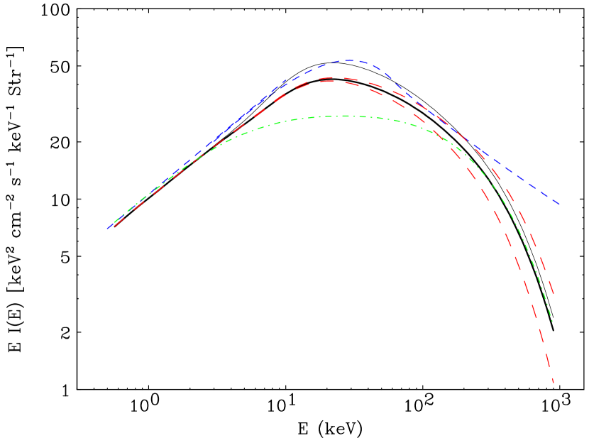
Figure 18: The integrated AGN spectra computed from our HXLF and the $N_{\rm H}$ function where several different conditions are compared with the observed CXB spectrum (uppermost dashed curves, blue). For the CXB spectrum we plot a power law with $\Gamma=1.4$ in the 0.5–10 keV band assuming the maximum normalization estimated by Barcons et al. (2000). In the 3–1000 keV band, the analytical formula by Gruber et al. (1999) is plotted with a normalization increased by 26% from the original value. Thick solid curve (black): the integrated spectrum of Compton-thin AGNs with Log $L_{\rm X}$ = 41.5–48 at $z<$5.0. Dot-dashed curve (green): that when the reflection component is not included. Dashed curves (red): those when the high energy cutoff is changed from $E_{\rm c}$= 500 keV to 400 keV (left) and 600 keV (right). Thin solid curve (black): that when the same number of Compton-thick AGNs with Log $N_{\rm H}$ =24–25 as those with Log $N_{\rm H}$ =23–24 are included.

At the faintest end we define a flux limited sample in the 2–8 keV band above $3.0\times 10^{-15}$ erg cm^-2 s^-1 (corresponding to $3.8\times 10^{-15}$ erg cm^-2 s^-1 in the 2–10 keV band for $\Gamma=1.4$) from the X-ray catalog of the Chandra Deep Survey North (CDFN) of a 1 Msec exposure (Brandt et al., 2001). We refer to the published results of optical identification by Barger et al. (2002) (we also utilize updated information given in Barger et al. 2003), including both spectroscopic and photometric redshifts. Following their definition, we divide the X-ray sample into two, the bright sample and the deep sample. The bright sample has a flux limit of $5\times 10^{-15}$ erg cm^-2 s^-1 (2–8 keV) within a 10 arcmin radius region around the field center covering an area of 294 arcmin². The deep sample is defined within a 6.5 arcmin radius, for which we limit the flux range brighter than $3.0\times 10^{-15}$ erg cm^-2 s^-1 (2–8 keV) to ensure high completeness. Finally redshifts of 57 sources (including 8 photometric redshifts) are known out of 61 sources. The completeness is 93%. From flux values listed in the Brandt et al. (2001) table we calculate flux hardness-ratio between the 0.5–2 and 2–8 keV bands, from which we estimate the absorption and luminosity, using an appropriate response of the ACIS instrument. We verified that our results are consistent with the absorption values derived by Barger et al. (2002) assuming $\Gamma=1.8$ (plotted in their Fig. 18). As argued in Barger et al. (2002) the X-ray sample is complete down to its flux limits over the defined area. Note that unlike the other samples, which are defined by count rate limits, this CDFN sample is defined by a true flux limit calculated by assuming a single power law with varying photon indices (see Brandt et al., 2001). We have taken this into account when correcting for selection biases of the sample.

2.4 Sample Summary

In summary, we have in total 247 hard-band selected AGNs covering the wide flux range from $10^{-10}$ to $3.8\times 10^{-15}$ erg cm^-2 s^-1 (2–10 keV), 49 AGNs from the HEAO1 surveys, 141 from ASCA, and 57 from Chandra with completeness of 100%, 97%, and 93%, respectively. AGNs at the overall flux range constitute a major part ($\;\buildrel>\over{\sim}\;$70%) of the CXB in the 2–10 keV band.

Our basic policy is to consider the HXLF of the entire AGN population we detected (except for a minor population of BL Lac objects) to avoid errors caused by further classification, which is not important in our discussion of the CXB origin as a whole. Nevertheless, for convenience of discussion, we classify each object into either a type-I or type-II AGN based on the X-ray or optical properties. We define X-ray type-II AGNs as those showing a best-fit absorption column density at the source redshift larger than $10^{22}$ cm^-2, and X-ray type-I AGNs as less absorbed sources. The method to obtain the column density is described in the next section.

From the optical data we basically define optical type-I AGNs as those showing broad emission lines and the rest as optical type-II AGNs. For the HEAO1 Part I AGNs we refer to the table compiled by Schartel et al. (1997) except NGC 2992, NGC 5506, and ESO 103, which we all classify as optical type-II. All the HEAO1 Part II sources are classified as optical type-I, including Seyfert 1.5, by referring mainly to the NED database. For the ASCA sources located at $z<0.6$, where the H$\beta$ region is covered in the optical spectroscopic observations (see A03), optical type-II AGNs are defined as those where broad H${\beta}$ lines are not significantly detected above 3$\sigma$. For those at $z>0.6$, we only classify those with broad emission lines of Mg II$\lambda$2800, C III]$\lambda$1909, and/or Ly$\alpha$ as optical type-I AGNs. For sources in the Lockman hole we adopt the same classification as in Lehmann et al. (2001). As for the CDFN sources, we refer to the last column in Table 1 of Barger et al. (2002) if there are broad emission lines. Thus, these optical classification schemes are not uniform for the whole sample and sometimes ambiguous, depending on the quality of the available optical spectrum and the wavelength coverage. In § 4.4 we discuss correlation between optical type-II AGNs and X-ray type-II AGNs.

Figure 1 shows the combined survey area as a function of limiting fluxes in the 2–10 keV band for the whole sample. The gap between $1.9\times 10^{-11}$ and $5\times 10^{-12}$ erg cm^-2 s^-1 (2–10 keV) is a result of setting the upper flux limit for the AMSS sample as mentioned above. Because the area is originally given as a function of count rate (except for the CDFN) in the survey band, we have assumed a power law with $\Gamma=$1.7, 1.6, and 1.4 for HEAO1, ASCA, and Chandra, respectively, in plotting this figure. To make an effective correction for completeness in the calculation of the HXLF, we modify the survey area by multiplying these completeness percentages, assuming that the luminosity/redshift distribution of unidentified sources is the same as that of identified sources. This assumption may not be always true because the incompleteness due to difficulty of optical identification is likely to be caused by non-random effects. Nevertheless, this does not cause any significant impacts on our conclusions presented in this paper within statistical uncertainties, thanks to the extremely high degree of the completeness.

3 Analysis

3.1 Goals

In this paper, we derive absorption column-density distribution function (“$N_{\rm H}$ function”) and the intrinsic hard X-ray luminosity function from our sample. The “intrinsic” luminosity (hereafter $L_{\rm X}$) means that it is corrected for an absorption (the value before being absorbed) in the rest frame 2–10 keV band. This enables us to discuss more directly the cosmological evolution of AGNs. Note that, in contrast, the SXLF by Miyaji et al. (2000a) is given in the observers’ frame by assuming a single photon index of 2 for all the sources. As a matter of fact, it has not been practical to correct for absorption of a ROSAT source because of the narrow bandpass limited below 2 keV. Consequently, however, the ROSAT results could be subject to biases against absorbed sources in that they miss them or significantly underestimate the true luminosity, in particular at lower redshifts where $k$-correction is not significant. The use of a hard-band selected sample itself greatly improves these disadvantages.

3.2 Absorption and Luminosity

To estimate the intrinsic luminosity ($L_{\rm X}$) with the best accuracy, we consider the spectrum of each object. After the photon index ($\Gamma$) and the absorption column density at the source redshift ($N_{\rm H}$) are determined, as described below, we convert the hard-band count rate into the absorption-corrected flux in the rest frame 2–10 keV band, $F_{\rm X}$, using the detector response. The Galactic absorption estimated from the H I observation (Dickey & Lockman, 1990) is taken into account field by field, even though its effect is mostly negligible. Then $L_{\rm X}$ is obtained as

$$L_{\rm X}=4\pi d_{\rm L}^{2}F_{\rm X},$$

where $d_{\rm L}$ is the luminosity distance. The statistical error in $L_{\rm X}$ arises from the error in the hard-band count rate itself as well as from those in the spectral parameters. The (propagated) errors in $L_{\rm X}$ for the AMSS sources are $<$20% and typically 5–15%, respectively. They correspond to an uncertainty of $<$0.1 in Log $L_{\rm X}$, which is negligible in our study.

Except for objects whose column density and photon index are independently determined from follow-up X-ray observations, we use the hardness ratio to estimate $N_{\rm H}$ or $\Gamma$. Here assumption must be made on the spectral shape because only one observational quantity is available. As an intrinsic spectrum before being absorbed, we assume a power law with an exponential cutoff, in the form of $E^{-\Gamma}{\rm exp}(\frac{E}{E_{\rm c}})$, with a Compton reflection component composed of reprocessed X-rays through cold, optically thick matter surrounding the emitter. We derive the corresponding $N_{\rm H}$ for each AGN if the observed hardness ratio is larger than the value expected from a “template spectrum”, representing a typical intrinsic spectrum of AGNs. Otherwise, we derive the corresponding $\Gamma$ value that accounts for the observed hardness ratio assuming no absorption.

Considering the overall results from spectral analysis of nearby AGNs (e.g., Nandra & Pounds, 1994; Turner et al., 1997; George et al., 1998), we adopt $\Gamma=1.9$ for the template spectrum. This value is also consistent with the mean photon index of the Lockman hole AGNs observed by XMM-Newton (Mainieri et al., 2002). The high energy cutoff ($E_{\rm c}$) of several hundred keV is found from bright Seyfert galaxies (e.g., Zdziarski et al., 1995). In this paper we assume $E_{\rm c}=$500 keV. Although the cutoff does not affect our determination of $N_{\rm H}$ and $L_{\rm X}$, it becomes important for predicting the contribution of AGNs to the CXB above 10 keV (§ 6.3). The reflection component is commonly detected in the X-ray spectra of nearby Seyfert galaxies (e.g., Nandra & Pounds, 1994), arising most likely from the accretion disk. To calculate the spectrum, we use the “pexrav” model (Magdziarz & Zdziarski, 1995) in the XSPEC package, assuming a solid angle of 2$\pi$, an inclination angle of cos$(i)$=0.5, and the Solar abundance for all elements. The ratio of the reflection component to the direct one is about 10% just below 7.1 keV (the K edge energy of cold iron atoms) and rapidly decreases toward lower energies (0.1% at 1 keV), while above 7.1 keV it has a maximum of about 70% around 30 keV, producing a “reflection hump”. This component makes the apparent slope in the 0.5–10 keV slightly harder than the intrinsic power law, depending on the redshift, but is almost negligible for determination of $N_{\rm H}$ from an individual spectrum. There are arguments that the relative strength of the reflection component (apparently) decreases with the luminosity (e.g., Lawson & Turner, 1997; Reeves & Turner, 2000), is smaller in radio loud AGNs than radio quite ones (Zdziarski et al., 1995), and may be even different between Seyfert 1 and Seyfert 2 galaxies (Zdziarski et al., 2000). For simplicity such possible dependence is neglected in this paper. We also ignore iron K emission lines in the spectra, whose contribution is less than few percent of the 2–10 keV continuum flux. These effects neglected here are not important for our main conclusions of the $N_{\rm H}$ function and the HXLF. Note that in the previous related papers (Akiyama et al., 2000, 2003) a single power law with $\Gamma=1.7$ was adopted for the template spectrum. This photon index was obtained from early X-ray missions such as HEAO1 and EXOSAT (e.g., Turner & Pounds, 1989), but is now considered to be in most cases an apparent slope affected by warm absorbers and a reflection hump (e.g., Nandra & Pounds, 1994). The choice of the $\Gamma$ value does not essentially affect our results. For comparison we will also show results of the $N_{\rm H}$ function obtained from the $\Gamma=1.7$ assumption.

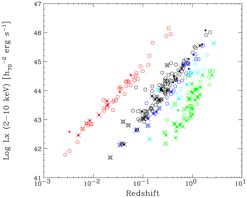
Figure 2: The redshift versus luminosity plot for our AGN sample (red: HEAO1, black: AMSSn+AMSSs, blue: ALSS, cyan: ASCA deep surveys, green: CDFN). The luminosity $L_{\rm X}$ is an “intrinsic” one in the rest frame 2–10 keV band before being absorbed. Dots: X-ray type-II AGNs (Log $N_{\rm H}$ $>$22). Crosses: optical type-II AGNs (with no significant broad emission lines).

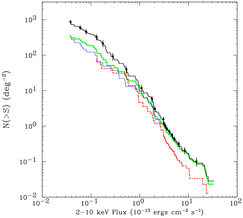
Figure 3: The observed log $N$ - log $S$ relation of the identified AGNs of our sample (uppermost line, black). The attached errors bar indicate $1\sigma$ Poisson errors in source counts. The thick sold line (green): X-ray type-I AGNs. The thin solid line (blue): AGNs at $z<0.8$. The dashed line (red): AGNs with Log $L_{\rm X}$ $\geq$44.5.

The redshift versus luminosity distribution of the whole sample is plotted in Figure 2. X-ray type-II AGNs are marked with dots and optical type-II AGNs with crosses. Figure 3 shows the log $N$ - log $S$ relations for the identified AGNs with different compositions; the total, X-ray type-I AGNs, AGNs at $z<0.8$, and those with $L_{\rm X}>10^{44.5}$ $h_{70}^{-2}$ erg s^-1. In plotting this, we use an observed (after absorption) flux in the 2–10 keV band for each source based on the best-fit spectral parameters as determined above. For the CDFN sources we simply use the original 2–8 keV fluxes given in Brandt et al. (2001) by multiplying a constant factor of 1.25 (i.e., assuming $\Gamma=1.4$) to convert them into 2–10 keV fluxes.

Figure 4(a) shows the observed $L_{\rm X}$ distribution of the whole sample compared with that of X-ray type-II AGNs (shaded histogram) and optical type-II AGNs (dashed). Figure 4(b) shows their redshift distribution. Figure 4(a) indicates that the fraction of optical type-II AGNs is not constant but larger in the lower luminosity range. The same tendency, though less evident, is also implied for X-ray type-II AGNs. It is important to note, however, that the observed ratio of absorbed AGNs does not give a correct estimate of the true fraction. In particular, there is a selection bias against detecting hard sources in a count-rate limited sample: at a given $L_{\rm X}$ and $z$, sources with larger $N_{\rm H}$ are more difficult to detect as they give smaller count rates. Also, because of statistical errors in the hardness ratio, the “observed” $N_{\rm H}$ distribution does not give the true distribution. To correct for these biases we perform quantitative analysis in § 4, by means of the maximum likelihood fit where the detector response is fully taken into account.

3.3 Principle of the Statistical Analysis

Below we explain the principle of how we determine the the $N_{\rm H}$ function and the HXLF by statistical analysis from our sample (for simplicity we do not consider the statistical error in the $N_{\rm H}$ determination at this moment). The luminosity function, representing the number density per unit comoving volume per Log $L_{\rm X}$ as a function of $L_{\rm X}$ and $z$, is expressed as

$$\frac{{\rm d}\Phi(L_{\rm X},z)}{{\rm dLog}L_{\rm X}}.$$

To describe the distribution of spectral parameters of AGNs at a given luminosity and redshift, we introduce the $N_{\rm H}$ function, $f(L_{\rm X},z;N_{\rm H}),$ a probability-distribution function for the absorption column-density. The $N_{\rm H}$ function has a unit of (Log $N_{\rm H}$)^-1 and is normalized to unity over a defined $N_{\rm H}$ region, that is

$$\int_{N_{\rm H,min}}^{N_{\rm H,max}}f(L_{\rm X},z;N_{\rm H}){\rm dLog}N_{\rm H}=1.$$ (1)

Generally, the form of the $N_{\rm H}$ function is dependent on the luminosity and the redshift. Similarly, we can also define the “photon index function” $g(L_{\rm X},z;\Gamma)$ per unit $\Gamma$ space. Throughout our paper we assume that there is no dependence of $f$ on the photon index $\Gamma$.

If these functions are modeled by analytical expressions, we can use the maximum likelihood (hereafter ML) method to search for the best-fit parameters and their statistical errors (see e.g., Miyaji et al., 2000a). The basic idea is to make the probability of finding the set of our observational results (i.e., distribution of the redshift, the count rate, and the spectrum) highest from the given survey conditions. Here we define the likelihood estimator $L$, to be minimized through the fitting, as

$$L=-2\sum_{i}{\rm ln}\frac{N(N_{{\rm H}i},\Gamma_{i},L_{{\rm X}i},z_{i})}{\int\int\int\int N(N_{\rm H},\Gamma,L_{{\rm X}},z){\rm dLog}N_{\rm H}{\rm d}\Gamma{\rm dLog}L_{\rm X}{\rm d}z}$$ (2)

where $i$ represents each object in our sample and $N$ is the expected number of detected sources per logarithm column density, per unit photon index, per logarithm luminosity, and per unit redshift. Here the expected number $N$ is calculated as

$$N(N_{\rm H},\Gamma,L_{{\rm X}},z)=f(L_{\rm X},z;N_{\rm H})g(L_{\rm X},z;\Gamma)\frac{{\rm d}\Phi(L_{\rm X},z)}{{\rm dLog}L_{\rm X}}d_{\rm A}(z)^{2}(1+z)^{3}c\frac{{\rm d}\tau}{{\rm d}z}(z)\sum_{j}A_{\rm j}(N_{\rm H},\Gamma,L_{\rm X},z)$$ (3)

where $d_{\rm A}^{2}$ and $\frac{{\rm d}\tau}{{\rm d}z}$ is the angular distance and the look back time per unit redshift, respectively, both are functions of $z$. The symbol $j$ represents each survey and $A_{\rm j}$ the survey area for a count rate expected from a source with $N_{\rm H}$, $\Gamma$, $L_{\rm X}$, and $z$, which can be calculated through the detector response and the luminosity distance. Eqs. (2) & (3) are a generalization of the formula (4) & (5) of Miyaji et al. (2000a) respectively towards the case where the spectrum of each source is taken into account in terms of $\Gamma$ and $N_{\rm H}$.

In the ML fit the 1$\sigma$ statistical error of each free parameter is obtained as a deviation from the best fit value when the $L$ value increases by 1.0 from its minimum. Unlike the $\chi^{2}$ fit, the minimum value itself does not have a meaning in statistics and therefore we cannot evaluate the absolute goodness of the fit. For the HXLF we use the two dimensional Kolgomorov-Smirnov test (2DKS test; Fasano & Franceschini 1987) applied for the luminosity-redshift distribution between the data and model: if the 2DKS probability is found to be larger than 0.2 then the model is considered acceptable within the statistics. Since the fit itself does not constrain the absolute normalization of the HXLF, we estimate it from the total number of observed sources.

As far as we use the above formula in the ML fit, the three ($N_{\rm H}$, photon index, and luminosity) functions are coupled with one another. In other words, ideally, all the parameters of the three functions must be constrained simultaneously. This is not practical, however, requiring huge computation time for the fit to converge. Hence, in this paper, we take an approximated, step by step approach as follows. (1) First, we determine the parameters of the $N_{\rm H}$ function using the observed values of the luminosity, redshift, and photon index of each source, without modeling the HXLF and the photon-index function by an analytical form (the delta-function approximation; see § 4.1 for details). (2) Next, we determine the model (and its best-fit parameters) of the HXLF through the ML fit by fixing the $N_{\rm H}$ function determined in the first step. For simplicity, we do not formalize the photon-index function but use $\Gamma=1.9$ for the calculation of $L$, which is found to be a sufficiently good approximation. The second step is repeated for several different parameters of the $N_{\rm H}$ function chosen within the statistical errors. We finally adopt the case when a combination of the HXLF and the $N_{\rm H}$ function meet observational constraints best, as described in § 5. The details of the first and second steps are described in the subsequent two sections.

4 The $N_{\rm H}$ function

4.1 Analysis Method

Below we derive the $N_{\rm H}$ function by representing the photon-index function and the HXLF with a superposition of the delta functions having a discrete peak at their observed values in the three dimensional space of ($\Gamma$, $L_{\rm X}$, $z$). In this approximation the formula of the likelihood estimator that constrains only the $N_{\rm H}$ function can be reduced to

$$L=-2\sum_{i}{\rm ln}\frac{f(L_{{\rm X}i},z_{i};N_{{\rm H}i})\sum_{j}A_{\rm j}(N_{{\rm H}i},\Gamma_{i},L_{{\rm X}i},z_{i})}{\int f(L_{{\rm X}i},z_{i};N_{{\rm H}})\sum_{j}A_{\rm j}(N_{{\rm H}},\Gamma_{i},L_{{\rm X}i},z_{i}){\rm dLog}N_{\rm H}}.$$ (4)

Here, the relative normalization of the delta function of each object is adjusted to give the minimum $L$ value in formula (2).

To make the best estimate of the $N_{\rm H}$ function, we also correct for bias arising from statistical errors in the hardness ratio in the ML fit. We derive $N_{\rm H}$ of each object at the source redshift from the best-fit hardness ratio value but its propagated error can be very large. As a result, the observed $N_{\rm H}$ function could be distorted from the true one: for example, because the hardness-ratio range corresponding to small absorptions (e.g., 20.5$<$ Log $N_{\rm H}$ = $<$21) becomes extremely narrow at high redshifts, the probability of finding objects in this $N_{\rm H}$ region is reduced when the hardness ratio is subject to statistical errors. Since it is difficult to make direct correction of the observed $N_{\rm H}$ function, we take the “forward analysis method” to the observed data to constrain the parameters of the (true) $N_{\rm H}$ function. Similarly to do a spectral fit with limited energy resolution, we introduce the “$N_{\rm H}$ response matrix function” $M_{i}(N^{0}_{{\rm H}},N_{\rm H})$, representing the probability of finding an observed value of $N_{\rm H}$ from the $i$-th object if it had a true absorption of $N^{0}_{\rm H}$. The matrix is normalized to unity between $20\leq{\rm Log}N_{\rm H}<24$. Then the $N_{\rm H}$ function term $f(L_{{\rm X}i},z_{i};N_{{\rm H}})$ in the above formula is replaced by

$$\int M_{i}(N^{0}_{\rm H},N_{{\rm H}})f(L_{{\rm X}i},z_{i};N^{0}_{{\rm H}}){\rm dLog}N^{0}_{\rm H}.$$ (5)

The $N_{\rm H}$ response matrix function is calculated for each object based on the observed count-rate errors in the two bands, using the hardness-ratio curve given as a function of $N_{\rm H}$ at the redshift of the object. For objects whose $N_{\rm H}$ and photon index are independently measured, we use the diagonal matrix assuming no statistical error.

4.2 Results

The histograms of Figure 5 show the observed $N_{\rm H}$ distribution (in units of number per bin) in different luminosity ranges (from the upper to lower panels, total, Log $L_{\rm X}$$<43$, $43\leq$ Log $L_{\rm X}$$<44.5$, and Log $L_{\rm X}$$\geq 44.5$), whereas those of Figure 6 are the “observed” $N_{\rm H}$ function (the probability distribution function in units of (Log $N_{\rm H}$)^-1, normalized to unity in Log $N_{\rm H}$ = 20 and 24) obtained only by correcting for the dependence of survey area on $N_{\rm H}$. As we have mentioned, these plots are inevitably subject to statistical errors in each $N_{\rm H}$ measurement, but are useful to make a first order estimate. Column densities smaller than Log $N_{\rm H}$ $<20$ are set to be Log $N_{\rm H}$ = 20 as an effective zero value. Considering large errors in the best-fit $N_{\rm H}$ value when Log $N_{\rm H}$ exceeds $\simeq$23, we here merge the two bins of Log $N_{\rm H}$ = 23–24.

In this paper we simply model the $N_{\rm H}$ function by a combination of three flat functions that have different values in the ranges of $N_{\rm H}<20.5$, $20.5\leq{\rm Log}N_{\rm H}<23$, and ${\rm Log}N_{\rm H}\geq 23$. We find that this form gives a sufficiently good explanation of the observed $N_{\rm H}$ distribution. Considering the limited statistics, we fix the ratio of the $N_{\rm H}$ function between Log $N_{\rm H}$ = 23–24 and Log $N_{\rm H}$ = 20.5–23, $\epsilon$, at 1.7, based on the $N_{\rm H}$ distribution of nearby, optically selected Seyfert 2 galaxies (Risaliti et al., 1999). We assume that $\epsilon$ is independent of the luminosity or redshift. Introducing the $\psi$ parameter, the fraction of absorbed AGNs (Log $N_{\rm H}$ = 22–24) to total AGNs (Log $N_{\rm H}$ $\leq$24), which is generally a function of both $L_{\rm X}$ and $z$, we can write the form of the $N_{\rm H}$ function as

$$f(L_{{\rm X}},z;N_{{\rm H}})=\begin{cases}2-\frac{5+2\epsilon}{1+\epsilon}\psi(L_{{\rm X}},z)&(20.0\leq{\rm Log}N_{\rm H}<20.5)\\ \frac{1}{1+\epsilon}\psi(L_{{\rm X}},z)&(20.5\leq{\rm Log}N_{\rm H}<23.0)\\ \frac{\epsilon}{1+\epsilon}\psi(L_{{\rm X}},z)&(23.0\leq{\rm Log}N_{\rm H}<24.0).\end{cases}$$ (6)

The comparison of the observed $N_{\rm H}$ functions in different luminosity ranges indicates that the fraction of absorbed (non-absorbed) sources is not constant, being smaller (larger) in higher luminosities. To express the luminosity dependence, we formalize $\psi$ by a linear function of Log $L_{\rm X}$ within a limited range:

$$\psi(L_{{\rm X}},z)={\rm min}[\psi_{\rm max},{\rm max}[\psi_{44}-\beta({\rm Log}L_{\rm X}-44),0]]$$ (7)

where

$$\psi_{max}=\frac{1+\epsilon}{3+\epsilon}.$$ (8)

Here we set the upper limit for $\psi$ ($\psi_{\rm max}$=0.574 if $\epsilon=1.7$) so that the value of the $N_{\rm H}$ function at Log $N_{\rm H}$ $<$20.5 does not become less than that of Log $N_{\rm H}$ $\geq$20.5. Introducing such “cutoff” is reasonable because a significant population of unabsorbed AGNs is known at Log $L_{\rm X}$ $\lower 2.15277pt\hbox{$\;\buildrel<\over{\sim}\;$}41$ (e.g., Terashima & Wilson, 2003). We note that the main results will be unchanged if the $\psi$ parameter is allowed to become larger than $\psi_{\rm max}$ at low luminosities. The redshift dependence of the absorption fraction is neglected. In fact, assuming that $\psi_{44}$ is proportional to $(1+z)^{\delta}$, we find that $\delta$ is consistent with zero within the statistical error (see also Figure 7(b)). Because our sample covers the wide $L_{\rm X}$- $z$ range combined from surveys with different flux limits, it is possible to constrain the luminosity dependence and the redshift dependence independently.

We perform the ML fit of the $N_{\rm H}$ function to our sample with the two free parameters $\psi_{44}$ and $\beta$. The results are summarized in Table 2. The results obtained with ($H_{0}$, $\Omega_{\rm m}$, $\Omega_{\lambda}$) = (50, 1.0, 0.0) and those with the $\Gamma=1.7$ assumption for the template spectrum are also given. To evaluate the goodness of the fit, the observed $N_{\rm H}$ distributions are compared with the model prediction (dashed line) in Figure 5. The 1-dimensional KS test yields matching probabilities higher than 0.70. It is recognized that the weak peak centered at Log $N_{\rm H}$ of $21.5-22$ is well reproduced through the $N_{\rm H}$ response matrix function. We find that $\beta$ is significantly larger than zero at $>3\sigma$ level, demonstrating the luminosity dependence of the absorbed-AGN fraction: the fraction of AGNs with Log $N_{\rm H}$ $>$22 to all GNs with Log $N_{\rm H}$ $<$24 decreases from 57${}^{+0}_{-5}$% at $L_{\rm X}=10^{43}$ $h_{70}^{-2}$ erg s^-1 to 37$\pm$5% at $L_{\rm X}=10^{45}$ $h_{70}^{-2}$ erg s^-1. In Figure 6 we plot the best-fit model of the $N_{\rm H}$ function. Figure 7(a) shows the averaged absorbed-AGN fraction derived in three luminosity ranges at all redshifts together with the best-fit model. Figure 7(b) shows its redshift dependence derived from the sample of $43<$ Log $L_{\rm X}$$<44.5$ with the best fit value calculated for its average luminosity. Although the statistical error is large, no significant redshift dependence is evident from our data. For comparison the same results obtained by assuming $\Gamma=1.7$ (with no reflection component) are shown in Figure 8(a) and (b).

4.3 Luminosity Dependence of the Fraction of X-ray Absorbed AGNs

Our result indicates that simple extension of the “unified scheme” to higher luminosity where the fraction of absorbed AGNs is assumed to be constant needs to be modified. We call this a “modified unified scheme”, which should be taken into account in population synthesis models of the CXB. This was originally suggested by Lawrence & Elvis (1982) and is consistent with the lack of type-II quasars seen in the ALSS sample as well as in the HEAO1 sample (Akiyama et al., 2000; Miyaji et al., 2003b).

To confirm this argument, we briefly discuss possible systematic effects caused by relying on a single hardness ratio without making detailed spectral analysis (which is practically impossible for most of ASCA sources). Firstly, we have ignored possible contribution of soft components over the absorbed continuum, such as a scattered component from the nucleus or a thermal emission by starburst activities. Basically, it leads us to underestimate the fraction of heavily absorbed sources. In a fixed energy band, the soft component becomes more important at lower redshifts. Thus, this effect only works to strengthen our argument because luminous objects are found at higher redshifts in a flux-limited sample. Secondly, we have assumed that the intrinsic power law index ($\Gamma$) does not depend on the luminosity. If there was correlation where the photon index is larger at higher luminosities then our result could be biased. We do not see such tendency, however, from our sources whose $\Gamma$ and $N_{\rm H}$ are independently measured. Moreover, as recognized from comparison between the $\Gamma=1.9$ and $\Gamma=1.7$ results (Figure 7 and 8), the luminosity dependence of the absorbed fraction is too large to be explained by a systematic difference in $\Gamma$ unless it is much larger than 0.2 between Log $L_{\rm X}$ = 43–44.5 and 44.5–46.5. These considerations support our conclusion that the absorbed-AGN fraction decreases with the luminosity.

We perform a more quantitative check of the overall effects of soft components on the result of the $N_{\rm H}$ function. According to the ASCA results of nearby Seyfert-II Galaxies (e.g., Turner et al., 1997), the relative normalization of the soft component is, in most cases, less than 5% of the absorbed continuum. We find that the best-fit parameters of the $N_{\rm H}$ functions do not change within errors even in the extreme case that all the sources have a 5% scattered component. Furthermore, even though the available data are limited, the number fraction of absorbed AGNs with strong soft components (i.e., those showing double peaks in the 0.5–10 keV band spectra) is small in a flux-limited sample regardless of flux levels. The X-ray spectroscopic study of the HEAO1 sample (Miyaji et al., 2003b) and the XMM-Newton result of the Lockman Hole sources (see Figure 3 of Mainieri et al. 2002) both indicate that it is only a few percent of the total sample (2 out of 49 and 1 (the source designated #50) out of $\approx$50, respectively).

In the analysis we ignore “Compton-thick” AGNs with column densities of Log $N_{\rm H}$ $>$24 assuming that such objects do not exist in our sample detected below 10 keV. However, the sample may contain some Compton-thick AGNs exhibiting reflection-dominated spectra below 10 keV. In this case we could underestimate not only $N_{\rm H}$ but also the intrinsic luminosity by more than an order of magnitude. Although the number density of Compton-thick AGNs detectable below 10 keV is poorly known at present, we infer it unlikely that it constitutes a significant fraction ($>$a few percent) in our sample, as indicated by the result of XMM-Newton and Chandra deep surveys (e.g., Mainieri et al., 2002; Barger et al., 2002). Indeed, such a small percentage is consistent with our estimate based on our population synthesis model (§ 6) when Compton-thick AGNs are included. Thus, as far as we discuss only Compton-thin AGNs, we conclude that our results should be reliable.

4.4 Fraction of optical type-II AGNs

It is possible to examine the fraction of optical type-II AGNs as a function of $N_{\rm H}$. One has to bear in mind, however, that the current definition of optical type-II AGNs in our sample is heterogeneous and is even dependent on the quality of the optical spectra because it is based on the detection “significance” of broad emission lines (§ 2.4). Hence, the results presented here should be taken as upper limits for the optical type-II AGN fraction. Basically they can be obtained by comparing the observed $N_{\rm H}$ distribution of optical type-II AGNs with that of the total AGNs because the survey area is common to both types at the same $N_{\rm H}$. Figure 9 shows the fraction of optical type-II AGNs, together with the observed histograms, as a function of $N_{\rm H}$ given in three luminosity ranges. The dashed line represents the best-fit analytical model determined in the whole luminosity range.

These figures indicate that there is good correlation between X-ray and optical classification of AGNs, as expected: almost all AGNs with Log $N_{\rm H}$ $>$23 are optical type-II AGNs, while there exists a small fraction of optical type-II AGNs in X-ray type-I AGNs. Apparently there seems to be luminosity dependence in the fraction of optical type-II AGNs. At the low luminosity range its fraction in AGNs in Log $N_{\rm H}$ $<$23 seems to be larger than the average. However, these results may be highly subject to observational biases: AGNs of lower luminosities are more likely to be contaminated by galaxies which make it more difficult to detect broad emission lines. Hence, we do not argue for the luminosity difference from these data.

5 The Hard X-ray Luminosity Function (HXLF)

Using the $N_{\rm H}$ function obtained in the previous section, we investigate the cosmological evolution of the HXLF of all AGNs including both type-I and type-II AGNs. We note again that our HXLF is defined for the absorption-corrected luminosity in the rest frame 2–10 keV band. In calculating the HXLF, unlike the $N_{\rm H}$ function, we exclude objects at $z<0.015$ to avoid possible effects of the local over-density and mis-estimate of their distances.

A practical goal here is to find an analytical expression that describes the overall HXLF data well, most preferably, a continuous function of $L_{\rm X}$ and $z$. Even though it does not have direct physical meaning, having such formula makes it very convenient to calculate various observational quantities and construct a population synthesis model. We search for a model that not only fits the HXLF data but also reproduces, when combined with the $N_{\rm H}$ function, other observational constraints, such as source counts at fainter fluxes than the flux limit in the 0.5–2 keV and 2–10 keV bands, the CXB intensity, and a redshift distribution of AGNs from other survey data, by extrapolating the form over the whole $L_{\rm X}$ and $z$ region. Here we refer to the result of direct source counts and fluctuation analysis obtained from the CDFN by Miyaji & Griffiths (2002). As for the absolute CXB intensity we adopt the best-fit value by Kushino et al. (2002), $6.4(\pm 0.7)\times 10^{-8}$ erg cm^-2 s^-1 Str^-1 in the 2–10 keV band (corresponding to a normalization of 9.7 keV cm^-2 s^-1 Str^-1 keV^-1 at 1 keV for a photon index of 1.4), derived from a wide area of 50 deg² with the ASCA GIS. This value is close to the median in the 90% confidence error region of a bayesian estimate by Barcons et al. (2000) using the ASCA and BeppoSAX results (10.0${}^{+0.6}_{-0.9}$ keV cm² s^-2 keV^-1 at 1 keV), but larger by $\simeq$20% than the HEAO1 measurement (Marshall et al., 1980) most probably because of cross-calibration error (see Barcons et al., 2000). The use of the ASCA value for self consistency of our analysis is justified, because the contribution of HEAO1 sources to the 2–10 keV CXB is less than 3% and the absolute flux calibration between ASCA and Chandra is accurate within 10% (see e.g., Barger et al., 2001).

Once the analytical expression is chosen for the HXLF, the free parameters are determined through the ML fit to our sample according to formula (2). After the ML fit, we check the consistency of the model with the observational constraints listed above and iterate these processes by changing the HXLF model or tuning the fixed parameters (including those of the $N_{\rm H}$ function within the errors). Since there are unlimited choices for an acceptable model within statistics, we try to select as simple expression as possible. Throughout the paper we adopt a smoothly-connected two power-law form to describe the present-day HXLF,

$$\frac{{\rm d}\Phi(L_{\rm X},z=0)}{{\rm dLog}L_{\rm X}}=A[(L_{\rm X}/L_{*})^{\gamma 1}+(L_{\rm X}/L_{*})^{\gamma 2}]^{-1}.$$ (9)

5.1 The PLE and the PDE

To begin with, we tried the two simplest models, the pure luminosity evolution (PLE) model and the pure density evolution (PDE) model. By introducing the evolution factor

$$e(z)=\begin{cases}(1+z)^{p1}&(z<z_{\rm c})\\ e(z_{\rm c})[(1+z)/(1+z_{\rm c})]^{p2}&(z\geq z_{\rm c}),\end{cases}$$ (10)

the PLE model is expressed as

$$\frac{{\rm d}\Phi(L_{\rm X},z)}{{\rm dLog}L_{\rm X}}=\frac{{\rm d}\Phi(L_{\rm X}/e(z),0)}{{\rm dLog}L_{\rm X}},$$ (11)

while the PDE model is

$$\frac{{\rm d}\Phi(L_{\rm X},z)}{{\rm dLog}L_{\rm X}}=\frac{{\rm d}\Phi(L_{\rm X},0)}{{\rm dLog}L_{\rm X}}e(z).$$ (12)

The best fit parameters are summarized in Table 3 together with the adopted parameters of the $N_{\rm H}$ function. It is interesting to note that we obtain the cutoff redshift above which the evolution terminates of $z_{\rm c}\simeq 1.2$ in both models. This value is smaller than the ROSAT result, $z_{\rm c}\simeq 1.6$ (Miyaji et al., 2000a). In terms of the 2DKS test performed over the whole $L_{\rm X}$-$z$ region, both models are found to be acceptable.

We find several difficulties, however, in adopting either the PDE or PLE model as our basic description of the HXLF that meets all the observational constraints. Firstly, the integrated intensity of AGNs with Log $L_{\rm X}$ = 41.5–48 and $z<5.0$ calculated from the best-fit PLE and PDE model overproduces the observed 2–10 keV CXB flux of Kushino et al. (2002) by a factor of 1.21 and 2.02, respectively. These values significantly exceed the 90% confidence region of the CXB intensity by Barcons et al. (2000). More seriously, the predicted 0.5–2 keV source counts in faintest flux levels largely overestimate the CDFN data by a factor of $>$2.6 at $S\simeq 7\times 10^{-17}$ erg cm^-2 s^-1. We find these problems cannot be resolved by tuning $p2$ within a reasonable range. These facts indicate that the number density of sources with smaller luminosities and/or at higher redshifts than our sample have to be reduced considerably from a simple extrapolation from the best-fit PLE or PDE model. Secondly, even though the significance is marginal, these models give relatively poor description of the HXLF data at $z>0.8$ as non-random residuals are left over a wide luminosity region. In the PLE, the model systematically underestimates all the data of Log $L_{\rm X}$ $<45$ at $z=0.8-1.6$ by a factor of $\simeq$2. Indeed, the 1-dimensional KS test performed for the (local) luminosity distribution in $z$=0.8–1.6 from 54 objects yields a matching probability of only 0.03 between the best-fit model and the data. The PDE model, on the other hand, underestimates the HXLF data of Log $L_{\rm X}$ $\geq 44.5$ at $z=1.6-3.0$ by a factor of $\simeq$4, resulting in a 1-dimensional KS probability of 0.02 (from 66 objects) for the redshift distribution in Log $L_{\rm X}$ $\geq 44.5$. These facts also suggest that the true evolution of the HXLF is more complex than the PLE or PDE. Actually, there is no physical reason why these simplest models should hold in the whole $L_{\rm X}$-$z$ range.

5.2 The LDDE model

To find a more sophisticated description of the HXLF, we consider a generalized luminosity-dependent density evolution (LDDE) model where, by definition, the evolution term in the formula (12) is not constant but a function of the luminosity. At first, to obtain an overall idea about the LDDE behavior, we derive the cutoff redshift ($z_{\rm c}$) and the slope ($p1$) in the evolution factor from two separate luminosity ranges, Log $L_{\rm X}$ $\geq 44.5$ and $44.5>$ Log $L_{\rm X}$ $\geq 43$. Fixing the other parameters at the best-fit values of the PDE in Table 3 (except $p2=-1.5$ for consistency with our final results derived below), we obtain ($z_{\rm c}$, $p1$) = (1.90${}^{+0.26}_{-0.31}$, 4.6${}^{+0.6}_{-0.5}$) and (1.01${}^{+0.06}_{-0.10}$, 4.0${}^{+0.5}_{-0.4}$), respectively (attached is the 1$\sigma$ error for a single parameter). This indicates that the cutoff redshift has strong luminosity dependence, being much smaller in lower luminosities, while the slope can be regarded to be constant within statistics. Note that this behavior is not the same as the LDDE model adopted by Miyaji et al. (2000a) for the SXLF, where $p1$ has luminosity dependence but $z_{\rm c}$ is set to be constant.

Based on this result, we determine $z_{\rm c}$ as a function of luminosity in finer bins, by fixing $p1$ at 4.2. The results are shown in Figure 10. In the luminosity regions smaller than Log $L_{\rm X}$ = 43 we obtain only lower limits, which are indicated by the arrows. The figure clearly reveals that $z_{\rm c}$ rapidly drops from $\simeq 1.9$ at Log $L_{\rm X}$ $\simeq 44.5$ toward lower luminosities. Because our sample has been made highly complete at all flux levels, the difference of $z_{\rm c}$ between luminosity ranges above and below Log $L_{\rm X}$ $\approx 44.5$ is a robust conclusion even if we consider the uncertainties on the redshift distributions of unidentified sources.

We finally find that the following LDDE model, where $z_{\rm c}$ is expressed by a power law of $L_{\rm X}$, well describes the current HXLF data as well as other observational constraints:

$$\frac{{\rm d}\Phi(L_{\rm X},z)}{{\rm dLog}L_{\rm X}}=\frac{{\rm d}\Phi(L_{\rm X},0)}{{\rm dLog}L_{\rm X}}e(z,L_{\rm X})$$ (13)

where

$$e(z,L_{\rm X})=\begin{cases}(1+z)^{p1}&(z<z_{\rm c}(L_{\rm X}))\\ e(z_{\rm c})[(1+z)/(1+z_{\rm c}(L_{\rm X}))]^{p2}&(z\geq z_{\rm c}(L_{\rm X}))\end{cases}$$ (14)

and

$$z_{\rm c}(L_{\rm X})=\begin{cases}z_{\rm c}^{*}&(L_{\rm X}\geq L_{a})\\ z_{\rm c}^{*}(L_{\rm X}/L_{a})^{\alpha}&(L_{\rm X}<L_{a}).\end{cases}$$ (15)

The best-fit parameters are summarized in Table 3 (we fix $z_{\rm c}^{*}$ and Log $L_{a}$ at 1.9 and 44.6, respectively, and leave $\alpha$ as a free parameter). In Figure 10 the best-fit function of $z_{\rm c}(L_{\rm X})$ is plotted by a dashed line. We set $p2=-1.5$ independently of the luminosity, so that (1) the model does not overproduce the source counts and that (2) it roughly describes the decline in number density of luminous AGNs revealed by the latest SXLF study (Hasinger, 2003).

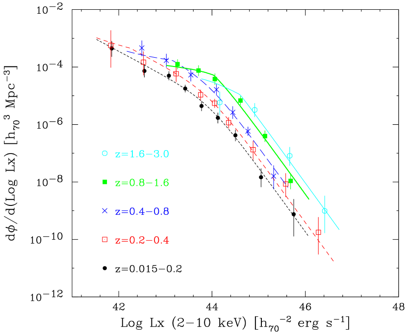
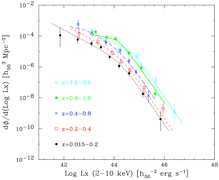
Figure 11: The intrinsic 2–10 keV hard X-ray luminosity function of AGNs. The curves represent our best-fit model (the LDDE model). The data are plotted according to the $N^{\rm obs}/N^{\rm mdl}$ method (Miyaji et al., 2001) with estimated 1$\sigma$ Poisson errors. The results are given in the five redshift bins of $z$=0.015–0.2 (short-dashed, black), 0.2–0.4 (medium-dashed, red), 0.4–0.8 (long-dashed, blue), 0.8–1.6(thick solid, green), and 1.6–3.0 (thin solid, cyan). Upper (a): ($H_{0}$, $\Omega_{\rm m}$, $\Omega_{\lambda}$) = (70$h_{70}$, 0.3, 0.7). Lower (b): ($H_{0}$, $\Omega_{\rm m}$, $\Omega_{\lambda}$) = (50$h_{50}$, 1.0, 0.0).

Figure 11 show the data of the HXLF in five redshift bins, $z$=0.015–0.2, 0.2–0.4, 0.4–0.8, 0.8–1.6, and 1.6–3.0 with the best-fit HXLF model calculated at the central redshift of each bin ($z$=0.1, 0.3, 0.6, 1.2, and 2.3, respectively). For plotting the HXLF we adopt the “$N^{\rm obs}/N^{\rm mdl}$ method” (Miyaji et al., 2001), where the best-fit model multiplied by the ratio between the number of observed sources and that of the model prediction in each $L_{\rm X}$-$z$ bin is plotted. Although model dependent, this technique is the most free from possible biases, compared with other methods such as the conventional $1/V_{a}$ method. The attached errors are estimated from Poissonian errors (1$\sigma$) in the observed number of sources according to the formula of Gehrels (1986).

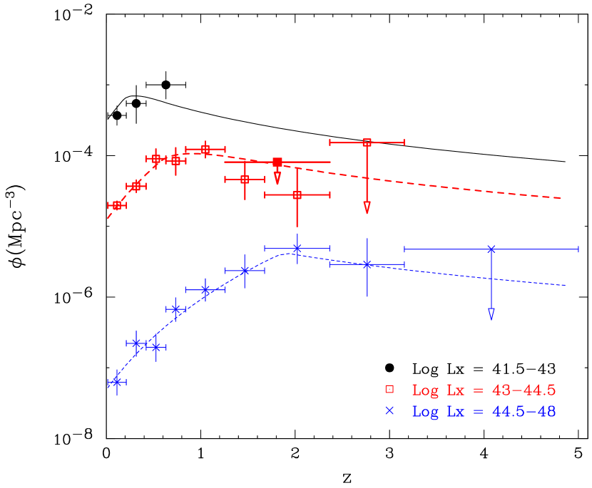
Figure 12: The comoving spatial density of AGNs as a function of redshift in three luminosity ranges, Log $L_{\rm X}$ =41.5–43 (upper, black), 43–44.5 (middle, red), 44.5–48 (lower, blue). The lines are calculated from the best-fit model of the HXLF. The error are $1\sigma$, while the long arrows denote the 90% upper limits (corresponding to 2.3 objects). The short arrow (marked with a filled square, red) corresponds to the 90% upper limit on the average spatial density of AGNs with Log $L_{\rm X}$ =43–44.5 at $z$=1.2–2.3 when all the unidentified sources are assumed to be in this redshift bin.

Figure 12 shows the same HXLF result in terms of the (comoving) spatial density as a function of redshift integrated in three luminosity regions (Log $L_{\rm X}$ = 41.5–43, 43–44.5, 44.5–48). The errors are 1$\sigma$ (same as in Figure 11), while the long arrows denote the 90% upper limits. It is clearly noticed that the cutoff redshift increases with the luminosity, and as a result the ratio of the peak spatial density to that of present day is much smaller for AGNs with Log $L_{\rm X}$ $<44.5$ than for more luminous AGNs. Note that these results are based on the “effective” correction for the sample incompleteness as described in § 2.4. To evaluate maximal errors due to the incompleteness, we calculate the same plot assuming that all the unidentified sources were located in a specific redshift as done by Cowie et al. (2003). We find that the incompleteness could affect any data points below $z<2.3$ only by a factor smaller than 2 except for those at $z>1.2$ in the Log $L_{\rm X}$ = 43–44.5 range. The short arrow shows the 90% upper limit on the average spatial density at $z=1.2-2.3$, which still gives a tight constraint.

5.3 Comparison with Observational Constraints

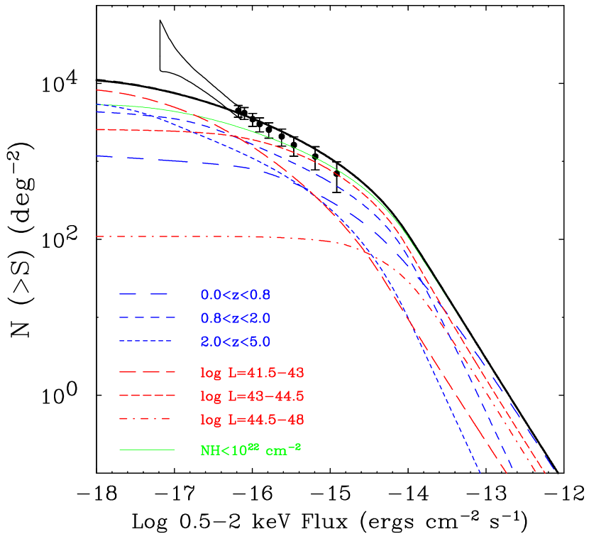
Figure 13: Predicted log $N$ - log $S$ relations from our model of the HXLF and the $N_{\rm H}$ function. The four figures correspond to different survey bands, (a) 0.5–2 keV, (b) 2–10 keV, (c) 5–10 keV, and (d) 10–30 keV. Black solid curve: the total contribution of only “Compton-thin” AGNs integrated Log $L_{\rm X}$ = 41.5–48 and $z<$5.0. Black dashed curve: when the same number of Compton-thick AGNs with Log $N_{\rm H}$ =24–25 as those with Log $N_{\rm H}$ =23–24 is included. Green curve: that of X-ray type-I AGNs. Blue (red) curves: contribution from different luminosity (redshift) ranges as indicated in the figure. The data points and enclosed regions in (a) and (b) are the constraint from the CDFN survey after Miyaji & Griffiths (2002). In the 5–10 keV band, the winding curve between Log $S$ = –14.6 and –13.4 and the data point at Log $S$ = –13.3 represents the XMM-Newton result of the Lockman hole and the BeppoSAX result, respectively (after Hasinger et al. (2001) and references therein).

Figure 13(a)–(d) shows the prediction of source counts (black solid curves) from the best-fit HXLF model and the $N_{\rm H}$ function in the four bands, 0.5–2 keV, 2–10 keV, 5–10 keV, and 10–30 keV. We also plot the source counts in the CDFN survey by Miyaji et al. (2000a) in the 0.5–2 keV and 2–10 keV bands, and that of XMM-Newton in the Lockman hole field by Hasinger et al. (2001) in the 5–10 keV band. It is verified that our model reproduces the observed 2–10 keV source counts above the flux limit, $3.8\times 10^{-15}$ erg cm^-2 s^-1. The predicted curve is, however, slightly below the 90% error region at the faintest fluxes $\lower 2.15277pt\hbox{$\;\buildrel<\over{\sim}\;$}10^{-15}$ erg cm^-2 s^-1. As we discuss later in §6.3, this discrepancy could be partially explained by Compton-thick AGNs with Log $N_{\rm H}$ =24–25. In the 5–10 keV band, the observed source counts is well reproduced by our model. In the 0.5–2 keV band, on the other hand, the predicted AGN contribution significantly underestimates the result of fluctuation analysis at fluxes of $8\times 10^{-18}-8\times 10^{-17}$ erg cm^-2 s^-1 (0.5–2 keV). This situation does not change even if we add a soft component with a relative normalization of 5% to the continuum for every AGN. Such discrepancy is also seen in the population synthesis model by Gilli, Salvati, & Hasinger (2001). As discussed by Miyaji & Griffiths (2002), this fact indicates the emergence of new populations, which could be attributable to normal galaxies (e.g., Ranalli, Comastri & Setti, 2003). They may also contribute to the faintest 2–10 keV source counts as well.

We confirm that our HXLF model can reproduce the redshift distribution of another hard-band selected sample containing other Chandra sources than used in the present analysis. Figure 14 shows comparison of the expected redshift distribution of AGNs (dashed histogram) with the actual data (solid) at a flux limit of $5\times 10^{-15}$ erg cm^-2 s^-1 in the 2–10 keV band taken from Gilli (2003). He compiled only spectroscopically identified sources in the Chandra deep field south (Giacconi et al., 2002), the CDFN, the Lockman Hole field, the Lynx field, and the Small Selected Area 13 field. The identifications were highly complete at this flux limit. He also excluded objects in certain redshift ranges where there are density spikes due to the underlying large-scale structure. The 1-dimensional KS test gives a matching probability of 0.75, which is well acceptable.

Finally we examine the consistency of our HXLF and the $N_{\rm H}$ function with the SXLF determined by ROSAT data. We refer to the SXLF by Miyaji et al. (2000a), which is calculated for all the soft X-ray selected AGNs (except BL Lac objects) without optical classification, as is in our case, but given for a luminosity in the observer 0.5–2 keV frame with no absorption correction. To make direct comparison, we calculate an expected SXLF by integrating contribution of AGNs with different intrinsic luminosities and column densities from our HXLF and $N_{\rm H}$ function. In this step we firstly compute the ROSAT PSPC count rate in the 0.5–2 keV band and then convert it into an “observed” luminosity assuming $\Gamma=2$, using the detector response.

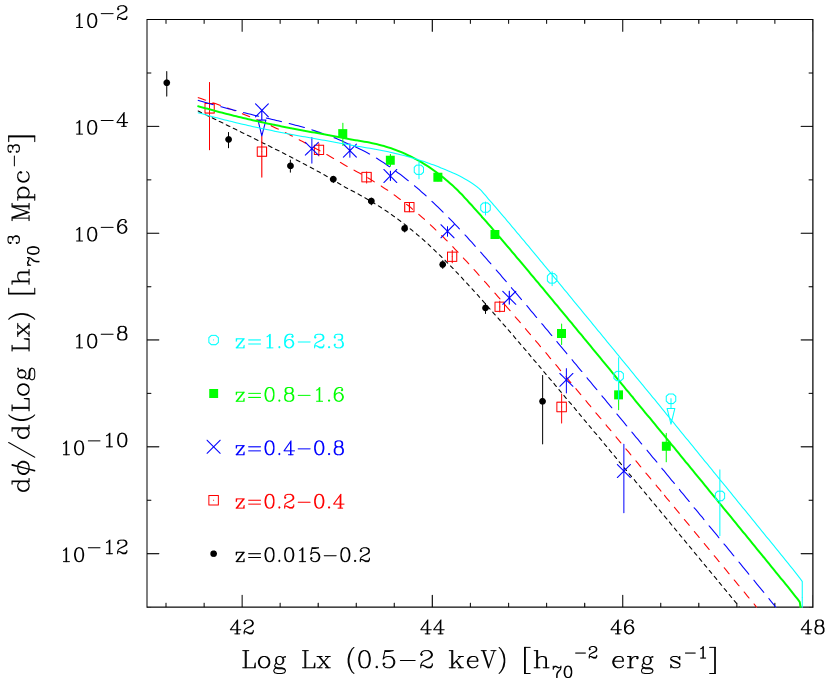
Figure 15: Comparison of a predicted SXLF from our HXLF and the $N_{\rm H}$ function (lines) with the ROSAT result (data points) by Miyaji et al. (2001), in the redshift bin of $z=$0.015–0.2 (short-dashed, black), 0.2–0.4 (medium-dashed, red), 0.4–0.8 (long-dashed, blue), 0.8–1.6 (thick solid, green), and 1.6–2.3 (thin solid, cyan).

Figure 15 shows the comparison between the observed SXLF data (points with error bars) and the prediction from the HXLF model (lines) in the redshift bins of $z$=0.015–0.2, 0.2–0.4, 0.4–0.8, 0.8–1.6, and 1.6–2.3. The data are taken from the numerical table of Miyaji et al. (2001) for the same cosmological parameters, ($H_{0}$, $\Omega_{\rm m}$, $\Omega_{\lambda}$) = (70, 0.3, 0.7). In spite of the fact that they are determined from completely independent surveys, we can see good agreement between the two results: they match within a factor of 2 or less than 2 $\sigma$ level. Because of $k$-correction more absorbed sources can fall into the soft X-ray band in higher redshifts, making the evolution appear to continue until a higher redshift than that of the HXLF. The effect is more important in the lower luminosity range because of the larger fraction of absorbed sources. This is probably the reason why the ROSAT SXLF is well described by the LDDE model with a constant cutoff redshift.

We note that the HXLF model tends to overestimates the SXLF at $z$=0.4–1.6 in the high luminosity range above Log $L_{\rm X}$ $\approx$ 45. A major reason is because the HXLF form we use is too simple, where a common two power-law form is assumed over the whole redshift range. In reality the slope $\gamma 2$ seems to be larger (and/or $L_{*}$ smaller) at these redshifts, as indicated from the SXLF data (it is also implied from our HXLF data; see Figure 11). This can be connected to the fact that the predicted source counts in the 0.5–2 keV band slightly overestimates the ROSAT result at fluxes below $\approx 10^{-13}$ erg cm^-2 s^-1 (Fig. 8 of Miyaji et al. 2000a). Similar tendency is also noticed in the hard band in the flux range of $10^{-12}-3\times 10^{-13}$ erg cm^-2 s^-1 (2–10 keV). Another possibility is that the current $N_{\rm H}$ function model may underestimate the fraction of absorbed sources, which could be dependent on redshift. Improvement of modeling of the HXLF and the $N_{\rm H}$ function with more complex forms to fully reflect these features is a future task, for which a combined analysis of the HXLF and SXLF would be useful. Nevertheless, the discrepancy at Log $L_{\rm X}$ $\;\buildrel>\over{\sim}\;$ 45 is not a serious problem in discussing the overall contribution to the CXB since the number density drops rapidly with $\propto L_{\rm X}^{-2.2}$.

6 Population Synthesis Model Update

Our results of the HXLF and the $N_{\rm H}$ function are extremely useful to establish a so-called population synthesis model of the CXB (e.g., Madau et al., 1994; Comastri et al., 1995; Gilli et al., 2001). The constructed model is most directly determined from the observations in the hard band and should update earlier works, which basically uses the result of the SXLF with assumptions for the $N_{\rm H}$ function. Nevertheless, we may still have to call it a “model” because below our flux limit it is based on extrapolation. Detailed modeling with many additional parameters is beyond the scope of this paper and we concentrate on basic consequences that are directly obtained from the HXLF and the $N_{\rm H}$ function. The best-fit parameters of the LDDE and of the $N_{\rm H}$ function in Table 3 for ($H_{0}$, $\Omega_{\rm m}$, $\Omega_{\lambda}$) = (70, 0.3, 0.7) are used. For the intrinsic AGN spectra we assume the “template spectrum” adopted in § 3.2 (i.e., $\Gamma=1.9$, a solid angle of 2$\pi$, inclination of cos$(i)$=0.5, cutoff energy $E_{\rm c}$ of 500 keV, and the Solar abundance). Several systematic effects caused by this assumption are briefly discussed in § 6.2.

In the calculation we integrate contribution of AGNs at $z<5$ within the luminosity range of Log $L_{\rm X}$ $>41.5$. Setting the luminosity limit is justified from comparison of our HXLF result with the upper limit at $0.1<z<1.0$ by Cowie et al. (2003): the AGN spatial density does not increase below the range of Log $L_{\rm X}$ = 41.5 and therefore its contribution to the CXB should be negligible compared to that of the total AGNs. We also neglect other populations such as clusters of galaxies, normal galaxies, and BL Lac objects, all of which have significantly softer spectra than the CXB spectrum. Results from previous surveys indicate that the overall contribution of these populations is very small affecting only the soft X-ray background. Although we basically consider “Compton-thin” AGNs with Log $N_{\rm H}$ $<24$ in this model, we finally discuss possible contribution of Compton-thick AGNs in § 6.3, which could have a significant contribution to the CXB above 10 keV.

6.1 The Composition of the CXB

In Figure 13 we also plot the predicted source counts of Compton-thin AGNs separately for different luminosity and redshift ranges: (red) for Log $L_{\rm X}$ = 41.5–43, 43–44.5, and 44.5–48 in $z<5.0$, and (blue) for $z$=0.0–0.8, 0.8–2.0, 2.0–5.0 in Log $L_{\rm X}$ = 41.5–48. The summed contribution of all the Compton-thin AGNs from Log $L_{\rm X}$$=41.5-48$ and $z<5.0$ is shown by the thick solid line (black), while that of only X-ray type-I AGNs is shown by the thin solid line (green). (The uppermost dashed line (black) corresponds to the case when Compton-thick AGNs are included with an extrapolation of the $N_{\rm H}$ function over Log $N_{\rm H}$ $>24$. See § 6.3.) The prediction in the 10–30 keV band can be examined with sensitive hard X-ray surveys by future missions such as Astro-E2, NeXT, Constellation-X, and XEUS.

Figure 16(a) and (b) shows the differential CXB intensity in the 2–10 keV band per unit Log $L_{\rm X}$ and redshift, given in different redshift and luminosity ranges, respectively. (The uppermost curves represent the case when Compton-thick AGNs are included.) It is seen that AGNs with Log $L_{\rm X}$ of $\simeq 43.8$ are the largest contributors to the 2–10 keV CXB as a total, although the peak luminosity decreases with the redshift. On the other hand, the contribution of AGNs per unit redshift is peaked at $z\approx 0.6$. Similarly, the peak redshift increases with the luminosity. These results can be fully understood as a consequence of the LDDE behavior of the HXLF. Figure 17 shows the same plots but in the 10–30 keV band. Since the effect of absorption is almost negligible in this band, these plots enable us to understand the CXB composition more directly. As recognized from the figure, the main part of the $E>10$ keV CXB is produced in the low redshift universe, peaked at $z\approx 0.5$. It is also seen that the contribution of Compton-thick AGNs becomes more important than in the energy band below 10 keV.

6.2 Reproduction of the Broad Band CXB Spectrum

A primary interest is whether our population synthesis model can reproduce the CXB spectrum in the broader band including energies above 10 keV. The uppermost dashed line (blue) in Figure 18 shows the representative form of the CXB spectrum in $EI(E)$, where $I(E)$ is the energy intensity per unit solid angle and $E$ the energy. We plot a power law with $\Gamma=1.4$ in the 0.5–10 keV range assuming the maximum normalization estimated by Barcons et al. (2000), 10.6 keV cm² s^-2 keV^-1 at 1 keV, and the empirical formula determined by Gruber et al. (1999) mainly from the HEAO1 A2 and A4 experiments, in the 3–1000 keV range. Before making detailed comparison, however, we have to recall possible systematic errors in the measurement of the CXB spectrum. Figure 2 of Gruber et al. (1999) suggests that there are still uncertainties of $>$5% in the measurement of the relative CXB shape in the 20–40 keV and $\;\buildrel>\over{\sim}\;$100 keV ranges. Also the spectrum of the extragalactic portion of the $E<$1 keV CXB is still controversial (e.g., Parmar et al., 1999). Besides this, there is an uncertainty of at least 16% (as large as 30% between different missions probably because of cross-calibration errors) in the absolute normalization of the CXB (see Barcons et al., 2000). In this figure we have increased the original normalization of Gruber et al. (1999) by 26% to connect to the 0.5–10 keV plot.

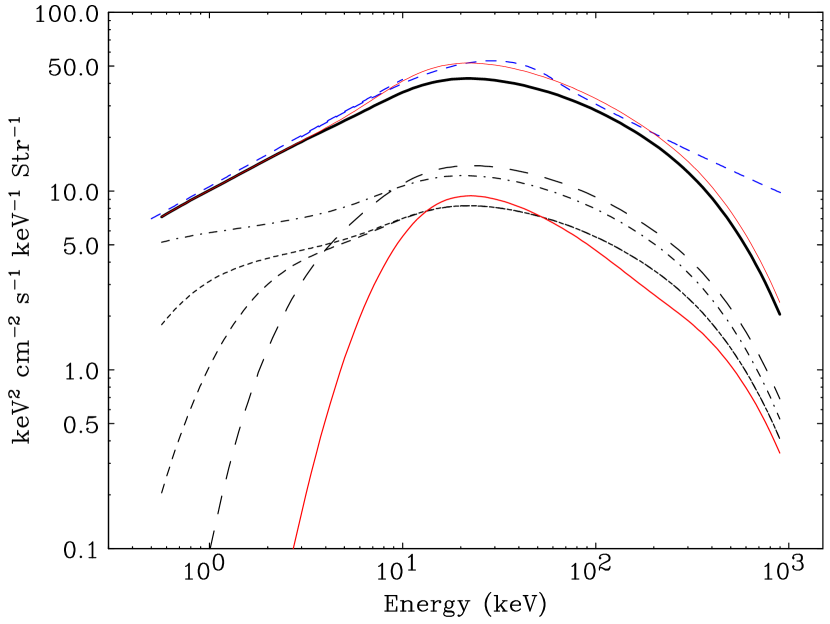
Figure 19: Contribution to the CXB from AGNs with different $N_{\rm H}$ ranges. Uppermost dashed curves (blue): the CXB spectrum same as Figure 18. Thick solid curve (black): the integrated spectrum of Compton-thin AGNs. Upper thin solid curve (red): the integrated spectrum when the same number of Compton-thick AGNs with Log $N_{\rm H}$ =24–25 as those with Log $N_{\rm H}$ =23–24 are included. Lower curves show separate contribution to the CXB from AGNs with Log $N_{\rm H}$ $<21$ (dot-dashed, black), Log $N_{\rm H}$ = 21–22 (short dashed), 22–23 (medium-dashed), 23–24 (long dashed), and 24–25 (solid, red).

The black thick curve in Figure 18 represents the integrated spectrum of Compton-thin AGNs with Log $L_{\rm X}$ = 41.5–48 at $z<5.0$ based on the template spectrum. Figure 19 shows contribution of AGNs with different column densities separately. The model spectrum reproduces the relative shape of the CXB within an accuracy of $\sim$20%. To illustrate effects of changing parameters of the template spectrum, we overplot the same results with the $E_{\rm c}$ value set to 400 keV (left red dashed curve) and 600 keV (right red dashed cure), keeping the other parameters the same. When $\Gamma=1.9$ is assumed, it is recognized that $E_{\rm c}$ cannot exceed $\approx$600 keV so as not to overproduce the CXB intensity above 100 keV. We also plot the extreme case by the green dot-dashed curve when the reflection component is absent. The comparison with the case of the template spectrum clearly indicates the importance of the reflection component in producing the hump structure of the CXB peaked at 30 keV, as was suggested by several authors (e.g., Fabian et al., 1990; Terasawa, 1991). The spectrum without a reflection component significantly underestimate the CXB intensity in the 5–100 keV range, producing a much broader peak than the CXB itself. Finally, we note the necessity of populations having non-thermal spectra (such as “blazars”) with an energy cutoff much higher than $\sim$ 1 MeV in reproducing the Gamma-ray background above a few hundred keV, even though they are minor populations in the X-ray band.

6.3 Contribution of Compton-Thick AGNs

A detailed inspection of Figure 18 suggests that the model based on the template spectrum slightly ($\approx$10–20%) underestimates the relative shape of the CXB spectrum around its peak intensity. As a possibility to explain this discrepancy, we consider contribution of Compton-thick AGNs. In fact, the result of Risaliti et al. (1999) suggests that there are roughly twice (1.6$\pm$0.6) as many AGNs with Log $N_{\rm H}$ $>24$ as those with Log $N_{\rm H}$ = 23–24. Accordingly, we simply extrapolate the $N_{\rm H}$ function above Log $N_{\rm H}$ $>24$ keeping the same normalization up to Log $N_{\rm H}$ = 26, assuming the “modified unified scheme” with no redshift dependence. This extrapolation may overestimate the true number of AGNs with Log $N_{\rm H}$ = 24–25, because in the $N_{\rm H}$ distribution of Risaliti et al. (1999) only upper limits of $N_{\rm H}$ are obtained for most (80%) of objects in this bin.

When the absorbing matter becomes Compton-thick, we have to take into account effects of Compton-scattering leading to significant decrease of the emitted flux even in the hard X-ray bands (Wilman & Fabian, 1999). Referring to their results of Monte Carlo calculation (with one Solar abundance), we approximately take account of this effect by multiplying energy dependent correction factors to the nominal absorbed spectrum. We neglect any contribution of objects with Log $N_{\rm H}$ $>$25 assuming that all X-rays are absorbed there before escaping. Inversely speaking, we cannot really constrain the number density of the whole Compton-thick populations by using the CXB intensity as a boundary condition.

The thin solid curve (black) in Figure 18 represents the integrated spectrum when Compton-thick AGNs are added according to the above assumption. In Figure 19 we plot the contribution from Compton-thick AGNs with a red solid line (the upper red solid line is the total of Compton-thin and thick AGNs). As expected, the inclusion of Compton-thick AGNs reduces the gap between the model and the CXB spectrum. The slight overestimate of the CXB around $\sim$100 keV is not an essential problem because it could be tuned by lowering $E_{\rm c}$. The spectral slope in the 2–10 keV band becomes slightly harder than a $\Gamma=1.4$ power law, although we have to keep in mind that we do not include any contribution of other “softer” populations here. The uppermost dashed curves (black) in Figure 13(a)–(d) represent the predicted source counts when Compton-thick AGNs are included. In the 2–10 keV band the total source counts are increased by about 20% at $S$ = $10^{-15}-10^{-16}$ erg cm^-2 s^-1, thus becoming more consistent with the data. In the 0.5–2 keV the source count is not affected at all in our assumption (i.e., no scattered component).

These results suggest that the presence of roughly equal number of Compton-thick AGNs of Log $N_{\rm H}$ = 24–25 as those with Log $N_{\rm H}$ = 23–24 is still consistent with the observations. We infer that the number density of AGNs with Log $N_{\rm H}$ = 24–25 assumed here roughly corresponds to its upper limit in order not to overproduce the 10–30 keV CXB, although this constraint depends on the shape of the template spectrum, in particular, on the relative strength of the reflection component (parameterized by the solid angle of the reflector). Finally we note that the reproductivity of the CXB spectrum is not yet perfect in the sense that the model peaks at a somewhat lower energy than that of the CXB. Here we do not pursue this discrepancy, however, considering many systematic uncertainties arising from the overly simple assumptions in our model (e.g., a single template spectrum, its spectral model, etc) as well as the measurement error (5–10%) in the CXB spectral shape itself.

7 Discussion

7.1 Summary of Our Work

Using the highly complete hard-band selected AGN sample covering the wide flux range of $10^{-10}-3.8\times 10^{-15}$ (2–10 keV), we have determined the $N_{\rm H}$ function and the intrinsic HXLF as a function of redshift and luminosity in the range of Log $L_{\rm X}$ = 41.5–46.5 and $z$ = 0–3. This means that we have directly revealed the evolution of most X-ray emitting, Compton-thin AGN populations that constitute a major part of the hard X-ray background in the 2–10 keV band. In other words, the CXB origin below 10 keV is now quantitatively solved by superposition of AGNs with different luminosities, redshifts, absorptions, and optical types. Our HXLF and $N_{\rm H}$ function, with an extrapolation to fainter fluxes than the flux limit, predicts various observational quantities that are consistent with currently available data. Based on these results we have constructed an observation based population synthesis model. Even though we make many simple assumptions, it predicts reasonably well the CXB spectrum in the 0.5–300 keV band. We find that the presence of a significant amount of Compton-thick AGNs as suggested in a local Seyfert 2 galaxy sample is consistent with the observations.

7.2 Implication from the $N_{\rm H}$ Function

7.2.1 Modified Unified Scheme

We have revealed that the $N_{\rm H}$ function has significant luminosity dependence in that the fraction of absorbed AGNs decreases with luminosity, while its redshift dependence is not significant. We call this picture “modified unified scheme” of AGNs, in contrast to the pure unified scheme where all the AGNs have the same geometrical structure regardless of its luminosity and redshift. A simple interpretation is that the opening angle of the dust torus is larger in more luminous AGNs. This may be attributable to the physical process that the high radiation pressure from a nucleus of luminous AGNs affects the physical structure of the torus.

Miyaji et al. (2000b) attempted to include this “deficiency of type II quasars” in their population synthesis model. However, Gilli, Risaliti, & Salvati (1999) found that their model involving this effect underestimates the 5–10 keV source count at $S\lower 2.15277pt\hbox{$\;\buildrel>\over{\sim}\;$}5\times 10^{-14}$ erg cm^-2 s^-1. Gilli et al. (2001) further explored models involving the cosmological evolution in the ratio of absorbed and unabsorbed AGNs. One of them included this “modified unified scheme”, but they disfavored this particular model because it underpredicted 2–10 keV source counts. Mainly because we now have a different form of the HXLF where the peak of the low luminosity AGNs (with abundant X-ray type-II AGNs) is at closer redshifts, contributed by the higher normalization of the absolute CXB intensity (see also e.g., Pompilio, La Franca & Matt 2000), we have now obtained a solution where this modified unified scheme is included, is consistent with hard (5–10 keV and 2–10 keV) source counts, and the cosmological evolution of the X-ray type II / type I ratio is not necessarily required.

It is an important question for galaxy formation theories whether the $N_{\rm H}$ function has any redshift dependence or not. For example, Franceschini et al. (2002) and Gandhi & Fabian (2003) suggest the possibility that the fraction of absorbed AGNs is significantly larger in $z\lower 2.15277pt\hbox{$\;\buildrel<\over{\sim}\;$}1$ than in higher redshifts, assuming a link of obscured AGNs to starburst galaxies. Our result derived from Compton-thin AGNs seems to rule out strong redshift dependence of the absorption fraction as proposed by these authors, confirming the argument by Gilli (2003). However, at least we do not have yet direct observational constraints on the fraction of the Compton-thick AGNs as a function of redshift. To fully establish our understanding of the whole AGN populations, further studies using a larger sample as well as sensitive hard X-ray surveys above 10 keV are necessary.

7.2.2 Fraction of Optical Type II AGNs in the Local Universe

Here we make a rough comparison on the fraction of optical type-II AGNs to check consistency of our picture with the results of optical surveys of local AGNs. The number ratio of Seyfert 1.8–2 galaxies to Seyfert 1–1.5 galaxies in the local universe is estimated to be 4.0$\pm$0.9 (Maiolino & Rieke, 1995). The sample of Risaliti et al. (1999), a sub-sample of the above one, has an average luminosity of Log $L_{\rm X}$ $\approx 43$ as seen in their Figure 1. At these luminosities, the fraction of AGNs with Log $N_{\rm H}$ = 22–24 to the total Compton-thin AGNs is $\simeq 0.57$ according to the $N_{\rm H}$ function (Figure 7). Estimates of the true fraction of type-II AGNs can be made only after knowing of the number density of the Compton-thick AGNs. Assuming that there exist 1.6 times as many Compton-thick AGNs as those with Log $N_{\rm H}$ = 23–24 (Risaliti et al., 1999), and that the fraction of optical type-II AGNs is 10%, 30%, and 100% at Log $N_{\rm H}$ $<$ 21, Log $N_{\rm H}$ = 21–22, and Log $N_{\rm H}$ $>$22, respectively (Figure 9), we expect that the ratio of optical type-II to optical type-I AGNs is 3.6. This estimate is consistent with the optical survey result.

7.3 Implication from the HXLF

7.3.1 Comparison with Previous Results of the HXLF

In § 5.3 we have already found that our HXLF result with the $N_{\rm H}$ function is consistent with the SXLF obtained from the largest sample of ROSAT surveys (Miyaji et al., 2000a). We here make comparison of our result with earlier works of the HXLF (we refer to the result with ($H_{0}$, $\Omega_{\rm m}$, $\Omega_{\lambda}$) = (50$h_{50}$, 1.0, 0.0) for consistency between different papers). Even though we find that the HXLF is best described by the LDDE model rather than other simpler forms, we here use the results of the PLE fit as reference when the cosmological evolution is discussed. Ceballos & Barcons (1996) calculated a local HXLF mostly from the HEAO1 Grossan sample. Boyle et al. (1998) derived a HXLF from a small number of ASCA sources and the Grossan sample, and more recently La Franca et al. (2002) obtain a HXLF, but of only optical type-I AGNs, from a combination of the 5–10 keV HELLAS survey, the ALSS, and the Grossan sample.

We confirm that the HXLF at $z<0.2$ (a sum of the optical type-I plus optical type-II AGNs) derived by Ceballos & Barcons (1996) and by Boyle et al. (1998) are consistent with our data within the statistical errors. Good agreement of the HXLF is confirmed in Log $L_{\rm X}$ $>44$ even though the error bars are small, simply reflecting the fact that we have used essentially the same HEAO1 sample for determination of the local HXLF in this luminosity range. Boyle et al. (1998) obtained the evolution factor $e(z)\propto(1+z)^{k}$ with $k=2.04^{+0.16}_{-0.22}$ assuming the PLE. The reason why it is apparently smaller than ours ($p1=2.7\pm 0.2$) is probably because the redshift cutoff above which the evolution terminates is not included in their analysis. On the other hand, since La Franca et al. (2002) uses an optical type-I AGN sample, the normalization they obtained is significantly smaller than our HXLF, which contains both optical type-I and optical type-II AGNs. We see the tendency that the discrepancy is larger in lower luminosities. This is expected from the luminosity dependence of the fraction of optical type-I AGNs. They obtain the PLE parameter of $p1=2.52$ at $z<1.39$ (and zero above then), which roughly agrees with our PLE-fit result ($p1=2.7\pm 0.2$ at $z<1.2$).

7.3.2 Comparison with Optical Luminosity Function of Quasars

In this subsection we compare our HXLF with an optical luminosity function (OLF) of broad line quasars, a sub class of AGNs (i.e., luminous, optical type-I AGNs). Here we refer to the results of the 2dF quasar survey by Boyle et al. (2000). They used more than 6000 quasars to construct the OLF in the $B$-band absolute magnitude of $-26<$ $M_{B}$ $<-23<$ at $z$=0.35–2.3, which was found to be well described by the PLE but with a different form for the evolution factor from formula (10). The comparison is not so trivial as with SXLFs because we must limit the HXLF to only optical type-I AGNs (or X-ray type-I AGNs approximately) to select the same population. Also, we need to assume a relation between $M_{B}$ and $L_{\rm X}$. The relation between an optical (ultra violet) luminosity and an X-ray luminosity is often parameterized by the $\alpha_{\rm OX}$ parameter defined as

$$\alpha_{\rm OX}\equiv-\frac{{\rm Log}(l_{\rm O}/l_{\rm X})}{{\rm Log}(\nu_{\rm O}/\nu_{\rm X})},$$

where $l_{\rm O}$ and $l_{\rm X}$ is the monochromatic luminosity (in units of erg s^-1 Hz^-1) at the rest-frame frequency $\nu$ of 2500$\AA$ and 2 keV, respectively. Many previous works indicate that $\alpha_{\rm OX}$ is correlated with the optical luminosity (luminous quasars being X-ray quiet), equivalent to the relation $l_{\rm X}\propto l_{\rm O}^{e}$ with $e\simeq 0.7-0.8$ (e.g., Kriss & Canizares, 1985; Avni & Tananbaum, 1986; Wilkes et al., 1994; Green et al., 1995; Yuan et al., 1998), although there are arguments against the presence of such an “intrinsic” correlation (La Franca et al., 1995; Yuan, Siebert, & Brinkmann, 1998b). The comparison between an OLF and an X-ray luminosity function provides an independent approach to constrain the $l_{\rm O}-l_{\rm X}$ relation (see Kriss & Canizares, 1985). Accordingly, we here search for an appropriate relation that realizes the best matching between the HXLF and the OLF.

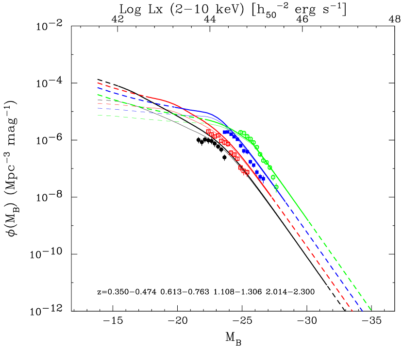
Figure 20: Comparison of the optical quasar luminosity function (data points) by Boyle et al. (2000) with our HXLF of X-ray type-I AGNs (thick lines) in the ($H_{0}$, $\Omega_{\rm m}$, $\Omega_{\lambda}$) = (50$h_{50}$, 1.0, 0.0) universe. From left to right, $z$=0.350–0.474 (black), 0.613–0.763 (red), 1.108–1.306 (blue), and 2.014–2.300 (green). The relation $\alpha_{\rm OX}=0.1152{\rm Log}l_{\rm O}-2.0437$ is assumed between the 2 keV and $2500\AA$ luminosities, corresponding to $l_{\rm X}\propto l_{\rm O}^{0.70}$ (see § 7.3.2 for details). The thin lines represent an estimated HXLF of only optical type-I AGNs. The dashed lines correspond to extrapolated regions where no X-ray sample exists.

We find that, if $e=1$ (or constant $\alpha_{\rm OX}$) is assumed, the apparent evolution of the HXLF of X-ray type-I AGNs becomes significantly slower than that of the OLF, whereas they become reasonably consistent with each other if $e\simeq 0.7$. This value is somewhat smaller than the previous result of the same approach by Boyle et al. (1993) using their SXLF ($e=0.88\pm 0.08$), but is consistent with the results obtained by Wilkes et al. (1994) and Vignali et al. (2003). Figure 20 shows the comparison of the quasar OLF (data points) by Boyle et al. (2000) with the prediction from the HXLF of X-ray type-I AGNs (thick lines) in the ($H_{0}$, $\Omega_{\rm m}$, $\Omega_{\lambda}$) = (50$h_{50}$, 1.0, 0.0) universe, where we have assumed the relation

$$\alpha_{\rm OX}=0.1152{\rm Log}l_{\rm O}-2.0437,$$

equivalent to $e=0.70$ and $\alpha_{\rm OX}=1.37$ at $M_{B}$ = –22.64 (or at $L_{\rm X}$ = $10^{44}h_{50}^{-2}$ erg s^-1). Corresponding $L_{\rm X}$ values are indicated in the upper label. For clarity we plot only the data in four redshift bins, $z$=0.350–0.474, 0.613–0.763, 1.108–1.306, and 2.014–2.300. The dashed lines of the HXLF represent extrapolated regions where no X-ray sample exists.

As noticed from the figure, they are consistent within a factor of 2 except for the smallest luminosity ranges ($M_{B}$ $>-23$) where the OLF is systematically smaller than the HXLF. The discrepancy may be (partially) due to selection effects as contamination of galaxy lights may affect the completeness of optical quasar surveys in low luminosity ranges. Indeed, our results on the fraction of optical type-II AGNs show the same tendency (Figure 9). To illustrate this effect, we also plot the HXLF of optical type-I AGNs with thin lines in Figure 20, assuming the approximated relation that the fraction of optical type-I AGNs in X-ray type-I AGNs decreases with the luminosity based on our result (§4.4). As expected, this reduces, though not perfectly, the discrepancy at $M_{B}$ $>-23$. More detailed comparison would require a larger sample for the HXLF as well as consideration of possible selection biases, which we leave for future studies. Finally we mention that, as recognized from Figure 20, the HXLF covers wider luminosity ranges than the OLF, demonstrating the importance of a combined analysis of X-ray surveys in various depths to understand the overall evolution of AGNs.

7.3.3 Accretion History of the Universe

In this paper we have shown that the cosmological evolution of the HXLF is best described by the LDDE model where the cutoff redshift increases with the luminosity. This means that the luminous AGNs (quasars) formed in earlier epochs than less luminous AGNs (such as Seyfert galaxies), consistent with the claims by Cowie et al. (2003) and Hasinger (2003). Our result directly constrains the formation history of super massive blackholes (SMBHs) in galactic centers not only for luminous, unobscured quasars that can be traced by optical surveys but also for less luminous or obscured AGNs, main contributors to the bulk of the CXB. Quantitative analysis of the growth curve of SMBHs and its relation to the local mass function of SMBHs are topics of a separate paper (Ueda et al., in preparation).

The accretion history of the SMBHs may have a strong link to the star formation history in their host galaxies. In this context, it is quite interesting to compare the evolution of the AGN luminosity density with that of the star forming rate density as a function of redshift. Kauffmann & Haehnelt (2000) showed that the optical luminosity function of quasars, its cosmological evolution, and the cosmic star formation history can be well reproduced simultaneously with some reasonable assumptions in semi-analytic models. Franceschini et al. (1999) pointed out that the history of luminosity density of luminous AGNs ($L_{\rm X}$ $>10^{44.25}h_{50}^{-2}$) derived from the ROSAT SXLF more closely resembles the formation history of early type galaxies rather than that of the total star-formation rate. This seems reasonable if we recall the tight correlation between the mass of a SMBH and the luminosity of a “spheroid component” of its host galaxy in the local universe (Magorrian et al., 1998). According to a more recent, semi-analytical model by Balland et al. (2003), the star formation of early type galaxies peaks earlier (at $z\approx 3$) than that of late type galaxies (at $z\approx 1.5$). This evolutionary difference is similar to our result that the number density of luminous AGNs (quasars) decays earlier than less luminous AGNs.

These facts may imply the following, first-order scenario. Luminous AGNs have lived in galaxies that have large spheroid components at present, such as ellipticals and S0s. Their SMBHs rapidly grew in accordance with strong star bursts that happened in early epochs of the universe (possibly as a result of mergers), followed by a rapid decrease of their activities after $z\lower 2.15277pt\hbox{$\;\buildrel<\over{\sim}\;$}2$. On the other hand, galaxies that now have only small spheroid (i.e., spirals) made star bursts relatively later and/or slower than early type galaxies, and accordingly the activity of smaller-mass (hence less luminous) AGNs has continued until recently ($z<1$). If the evolutionary history by Balland et al. (2003) is the case, the star forming activity peaks at somewhat earlier epochs (at $z\approx 3$ for early type and $z\approx 1.5$ for late type galaxies) than the AGN activities of the same population in the above scenario (at $z\approx 2$ and $z\approx 0.6$, respectively). This would imply that the AGN activity of a galaxy occur not in the same but a later phase than the major star burst. We note, however, that an apparently weak AGN could be either a small mass BH or a high mass BH with a small accretion rate, making the actual story more complex. Obviously we need discussion combined with the mass function of SMBHs, which shall be left for future work.

8 Conclusion

1. From a combination of hard X-ray surveys above 2 keV with various depths and area performed with HEAO1, ASCA, and Chandra, we have constructed a highly complete AGN sample consisting of 247 sources in the wide flux range covering $10^{-10}-3.8\times 10^{-15}$ erg cm^-2 s^-1 (2–10 keV). This provides us with an ideal opportunity to unambiguously trace the evolution of both type-I and type-II AGNs in the range of Log $L_{\rm X}$ of 41.5–46.5 and $z=0-3$.

2. For our purpose, we develop an extensive method of calculating the intrinsic (before-absorption) hard X-ray luminosity function (HXLF) and the absorption ($N_{\rm H}$) function. This utilizes the maximum likelihood method fully correcting for observational biases with consideration of the X-ray spectrum of each source.

3. We find that the fraction of absorbed AGNs decreases with increasing luminosities, while the redshift dependence is not significant within our data. This result requires modification of the pure “unified scheme” of AGNs.

4. The HXLF shows different cosmological evolution between luminous and less luminous AGN in terms of the cutoff redshift $z_{\rm c}$ above which density evolution terminates: quasars formed earlier than lower luminosity AGNs. We find that the HXLF is well described with the luminosity dependent density evolution model where $z_{\rm c}$ decreases from $\simeq 1.9$ at Log $L_{\rm X}$ $\lower 2.15277pt\hbox{$\;\buildrel>\over{\sim}\;$}45$ to $\approx 0.8$ at Log $L_{\rm X}$ $\simeq 43.5$.

5. The combination of the HXLF and the $N_{\rm H}$ function enables us to construct a purely observation based population synthesis model of the CXB. The model predicts observational constraints fairly well, including source counts at faintest fluxes available in the ranges of 0.5–10 keV, the 0.5–2 keV luminosity function determined with ROSAT, and the broad band spectra of the CXB in the 0.5–300 keV band. The presence of roughly the same number of Compton-thick AGNs with Log $N_{\rm H}$ =24–25 as those with Log $N_{\rm H}$ =23–24 is consistent with the observations. Our results are also consistent with the number ratio between Seyfert 1 and Seyfert 2 galaxies in the local universe and with the optical luminosity function of quasars at $z=$0.35–2.3 with reasonable assumptions.

6. These results give a basis of observational constraints on the accretion history of the universe, i.e., the formation history of super massive black holes that reside in most of galaxies.

Figure 1: The total survey area as a function of a 2–10 keV flux for our whole sample.

Figure 4: left (a): The luminosity distribution of the whole sample, compared with that of X-ray type-II AGNs (shaded histogram) and that of optical type-II AGNs (dashed histogram). right (b): The redshift distribution of the same samples as (a).

Figure 5: The observed $N_{\rm H}$ distributions (with 1$\sigma$ Poisson errors) are compared with the prediction from the best-fit $N_{\rm H}$ function (dashed histogram) in different luminosity ranges (from upper to lower panels: total, Log $L_{\rm X}$ $<$ 43, 43 $\leq$ Log $L_{\rm X}$ $<$ 44.5, and Log $L_{\rm X}$ $\geq$ 44.5).

Figure 6: The observed $N_{\rm H}$ functions of our sample (with 1$\sigma$ statistical errors) in different luminosity ranges (same as Figure 5.) The dashed lines represent the best-fit model of the $N_{\rm H}$ function, obtained by correcting for biases due to the statistical error in $N_{\rm H}$.

Figure 7: The fraction of absorbed AGNs with Log $N_{\rm H}$ $>22$ to all AGNs with Log $N_{\rm H}$ $<24$, given as as a function of (left :a) luminosity and (right :b) redshift. The data points in (b) are calculated from AGNs in the luminosity range of Log $L_{\rm X}$ = 43–44.5. Dashed lines represent the best fit model of the $N_{\rm H}$ function.

Figure 8: The same as Figure 7 obtained when a power law of $\Gamma=1.7$ with no reflection component is assumed for the template spectrum.

Figure 9: Upper panels: the fraction of optical type-II AGNs given as a function of $N_{\rm H}$. Lower panels: observed histogram of the total sample compared with that of only optical type-II AGNs (shaded histogram). The three figures correspond to different luminosity ranges (left: Log $L_{\rm X}$ $<$43, center: 43$\leq$ Log $L_{\rm X}$ $<$44.5, right: Log $L_{\rm X}$ $\geq$44.5). The dashed line represents the best-fit analytical model determined in the whole luminosity range.

Figure 10: The cutoff redshift ($z_{\rm c}$) of the AGN density evolution determined as a function of the luminosity. Error bars correspond to 1$\sigma$ errors obtained through the ML fit. The arrows denote 90% lower limits. The position of the marker corresponds to the mean luminosity in each region. The dashed line is the best-fit model used in our HXLF formula.

Figure 14: The redshift distribution of the hard-band selected sample compiled by Gilli (2003) at a flux limit of $5\times 10^{-15}$ in the 2–10 keV band. The dashed histogram is the prediction from our model.

Figure 16: Differential contribution of AGNs to the 2–10 keV CXB intensity as a function of (upper: a) luminosity and (lower: b) redshift, based on the best-fit model of the HXLF and the $N_{\rm H}$ function. The dashed lines show contribution from different redshift or luminosity ranges as indicated in the figures. The uppermost curves correspond to the case when the same number of Compton-thick AGNs with Log $N_{\rm H}$ =24–25 as those with Log $N_{\rm H}$ =23–24 are included.

Figure 17: The same as Figure 16 but calculated for the 10–30 keV CXB.

Table 1: Surveys Used in the Analysis

Survey	No. of	Flux Limit (2–10 keV)	Reference
	Id. AGNs	[erg cm-2 s-1]
HEAO1 A2	28	$2.7\times 10^{-11}$	Piccinotti et al. (1982)
HEAO1 MC-LASS	21	$1.9\times 10^{-11}$	Grossan (1992)
AMSSn	74	$3.1\times 10^{-13}$	Akiyama et al. (2003)
AMSSs	20	$3.1\times 10^{-13}$	Akiyama et al., in prep.
ALSS	30	$1.2\times 10^{-13}$	Akiyama et al. (2000)
ASCA Lockman	12	$3.8\times 10^{-14}$	Ishisaki et al. (2001)
ASCA Lynx	5	$5.0\times 10^{-14}$	Ohta et al. (2003)
CDFN	57	$3.8\times 10^{-15}$	Barger et al. (2002)

Table 2: The Best Fit Parameters of the $N_{\rm H}$ function

Photon Index	1.9	1.9	1.7
Reflection	yes	yes	no
($H_{0}$, $\Omega_{\rm m}$, $\Omega_{\lambda}$)	(70,0.3,0.7)	(50,1.0,0.0)	(70,0.3,0.7)
$\epsilon$	1.7 (fixed)	1.7 (fixed)	1.7 (fixed)
$\psi_{44}$	0.47$\pm$0.03	0.48${}^{+0.04}_{-0.02}$	0.41$\pm$0.03
$\beta$	0.10${}^{+0.04}_{-0.03}$	0.09${}^{+0.06}_{-0.03}$	0.12$\pm$0.03

Note. — Errors are 1$\sigma$ for a single parameter.

Table 3: The Best Fit Parameters of the HXLF models

Model	PLE	PDE	LDDE	LDDE
($H_{0}$, $\Omega_{\rm m}$, $\Omega_{\lambda}$)	(70,0.3,0.7)	(70,0.3,0.7)	(70,0.3,0.7)	(50,1.0,0.0)
$A$	$14.1\pm 1.0$	$2.64\pm 0.18$	$5.04\pm 0.33$	$1.92\pm 0.13$
Log $L_{*}$	43.66$\pm$0.17	44.11$\pm$0.23	43.94${}^{+0.21}_{-0.26}$	44.23$\pm$0.19
$\gamma_{1}$	0.82$\pm$0.13	0.93$\pm$0.13	0.86$\pm$0.15	0.86$\pm$0.13
$\gamma_{2}$	2.37$\pm$0.16	2.23$\pm$0.15	2.23$\pm$0.13	2.36$\pm$0.15
$p1$	2.70${}^{+0.17}_{-0.25}$	4.20$\pm$0.32	4.23$\pm$0.39	4.43${}^{+0.34}_{-0.27}$
$p2$	0.0 (fixed)	0.0 (fixed)	$-1.5$ (fixed)	$-1.5$ (fixed)
$z_{\rm c}$ (or $z_{\rm c}^{*}$)	1.15${}^{+0.20}_{-0.07}$	1.14${}^{+0.13}_{-0.16}$	1.9 (fixed)	1.9(fixed)
Log $L_{a}$	$\cdots$	$\cdots$	44.6 (fixed)	44.89 (fixed)
$\alpha$	$\cdots$	$\cdots$	0.335$\pm$0.070	0.243$\pm$0.040
$\epsilon$	1.7	1.7	1.7	1.7
$\psi_{44}$	0.5	0.5	0.5	0.529
$\beta$	0.1	0.1	0.1	0.1
$P_{\rm 2DKS}$	0.58	$>$0.9	$>$0.9	$>$0.9
$I_{\rm 2-10}$	1.21	2.02	0.96	0.97
$N(>S_{0.5-2})$	2.6	6.1	0.94	0.98

Note. — Errors are 1$\sigma$ for a single parameter.

References

- Akiyama et al. (2000) Akiyama, M., et al. 2000, ApJ, 532, 700
- Akiyama et al. (2002) Akiyama, M., Ueda, Y., & Ohta, K. 2002, ApJ, 567, 42
- Akiyama et al. (2003) Akiyama, M., et al. 2003, ApJS, in press (astro-ph/0307164) (A03)
- Avni & Tananbaum (1986) Avni, Y., & Tananbaum, H. 1986, ApJ, 305, 83
- Balland et al. (2003) Balland, C., Devriendt, J.E.G, & Silk, J 2003, MNRAS, 343, 107
- Barcons et al. (2000) Barcons, X., Mateos, S., & Ceballos, M.T. 2000, MNRAS, 316, L13
- Barger et al. (2001) Barger, A.J., Cowie, L.L., Mushotzky, R.F., & Richards, E.A. AJ, 121, 662
- Barger et al. (2002) Barger, A.J., et al. 2002, AJ, 124, 1839
- Barger et al. (2003) Barger, A.J., et al. 2003, AJ, 126, 632
- Boldt (1987) Boldt, E., 1987, Phys. Rep., 316, 215
- Boyle et al. (1993) Boyle, B.J., et al. 1993, MNRAS, 260, 49
- Boyle et al. (1998) Boyle, B.J., et al. 1998, MNRAS, 296, 1
- Boyle et al. (2000) Boyle, B.J., et al. 2000, MNRAS, 317, 1014, 2000
- Brandt et al. (2001) Brandt, W.N., et al. 2001, AJ, 122, 2810
- Burke et al. (1991) Burke, B.E., Mountain, R.W., Harrison, D.C., Bautz, M.W., Doty, J.P., Ricker, G.R., & Daniels, P.J. 1991, IEEE-ED, 38, 1069
- Ceballos & Barcons (1996) Ceballos, M.T., & Barcons, X. 1996, MNRAS, 282, 493
- Comastri et al. (1995) Comastri, A., Setti, G., Zamorani, G., & Hasinger, G. 1995, A&A, 296, 1
- Cowie et al. (2003) Cowie, L.L., et al. 2003, ApJ, 584, L57
- Dickey & Lockman (1990) Dickey, J.M., & Lockman, F.J. 1990, ARA&A, 28, 215
- Fabian et al. (1990) Fabian, A.C., et al. 1990, MNRAS, 242, 14
- Fabian & Barcons (1992) Fabian, A.C., & Barcons, X., 1992, ARA&A, 316, 429
- Fasano & Franceschini (1987) Fasano, G., & Franceschini, A., 1987, MNRAS, 225, 155
- Franceschini et al. (1999) Franceschini, A. et al. 1999, MNRAS, 310, L5
- Franceschini et al. (2002) Franceschini, A., Braito, V., & Fadda, D. 2002, MNRAS, 335, L51
- Gandhi & Fabian (2003) Gandhi, P., & Fabian, A.C. 2003, MNRAS, 339, 1095
- Gehrels (1986) Gehrels, N. 1986, ApJ, 303, 336
- George et al. (1998) George, I.M., et al. 1998, ApJS, 114, 73
- Giacconi et al. (2002) Giacconi, R., et al. 2002, ApJS, 139, 369
- Gilli et al. (1999) Gilli, R., Risaliti, G., Salvati, M. 1999, A&A, 347, 424
- Gilli et al. (2001) Gilli, R., Salvati, M., Hasinger, G. 2001, A&A, 366, 407
- Gilli (2003) Gilli, R. 2003, in New X-ray Results from Clusters of Galaxies and Black Holes, eds. C. Done, E.M. Puchnarewicz, M.J. Ward, Advances in Space Research, in press (astro-ph/0303115)
- Green et al. (1995) Green, P.J., et al. 1995, ApJ, 450, 51
- Grossan (1992) Grossan, B., 1992, PhD thesis, MIT
- Gruber et al. (1999) Gruber, D.E., et al. 1999, ApJ, 520, 124
- Hasinger et al. (2001) Hasinger, G., et al. 2001, A&A, 36,5 L45
- Hasinger (2003) Hasinger, G. 2003, in the 13th Annual Astrophysics Conference in Maryland: The Emergence of Cosmic Structure, eds. Stephen S. Holt & Chris Reynolds; AIP Conf.Proc. 666 (2003) 227-236 (astro-ph/0302574)
- Ishisaki et al. (2001) Ishisaki, Y., et al. 2001, PASJ, 53, 445
- Jones et al. (1997) Jones, L.R., et al. 1997, MNRAS, 285, 547
- Kauffmann & Haehnelt (2000) Kauffmann, G., & Haehnelt, M. 2000, MNRAS, 576, 311
- Kriss & Canizares (1985) Kriss, G., & Canizares, C.R. 1985, ApJ, 297, 177
- Kushino et al. (2002) Kushino, A., et al. 2002, PASJ, 54, 327
- La Franca et al. (1995) La Franca, F., et al. 1995, A&A, 299, 19
- La Franca et al. (2002) La Franca, F., et al. 2002, ApJ, 570, 100
- Lawrence & Elvis (1982) Lawrence, A. & Elvis, M. 1982, ApJ, 256, 410
- Lawson & Turner (1997) Lawson, A.J., & Turner M.J.L. 1997, MNRAS, 288, 920
- Lehmann et al. (2001) Lehmann, I., et al. 2001, A&A, 371, 833
- Maccacaro et al. (1991) Maccacaro, T. et al. 1991, ApJ, 374, 117
- Madau et al. (1994) Madau, P., Ghisellini, G., Fabian, A.C. 1994, MNRAS, 270, L17
- Magdziarz & Zdziarski (1995) Magdziarz, P., & Zdziarski, A.A. 1995, MNRAS, 273, 837
- Magorrian et al. (1998) Magorrian, J., et al. 1998, AJ, 115, 2285
- Mainieri et al. (2002) Mainieri, V., et al. 2002, A&A, 393, 425
- Maiolino & Rieke (1995) Maiolino, R., & Rieke, G.H. 1995, ApJ, 454, 95
- Malizia et al. (2002) Malizia, A, et al. 2002, A&A, 394, 801
- Marshall et al. (1980) Marshall, F.E., et al. 1980, ApJ, 1980, 235, 4
- Miyaji et al. (2000a) Miyaji, T., Hasinger, G., & Schmidt, M. 2000a, A&A, 353, 25
- Miyaji et al. (2000b) Miyaji, T., Hasinger, G., & Schmidt, M. 2000b, Advances in Space Research, 25, 827
- Miyaji et al. (2001) Miyaji, T., Hasinger, G., & Schmidt, M. 2001, A&A, 369, 49
- Miyaji & Griffiths (2002) Miyaji, T., & Griffiths, R.E. 2002, ApJ, 564, L5
- Miyaji et al. (2003a) Miyaji et al., 2003, PASJ, 55, L11
- Miyaji et al. (2003b) Miyaji et al., 2003b, in preparation
- Nandra & Pounds (1994) Nandra, K. & Pounds, K.A. 1994, MNRAS, 268, 405
- Ohashi et al. (1996) Ohashi, T., et al. 1996, PASJ, 48, 157
- Ohta et al. (2003) Ohta, K., et al. 2003, ApJ, in press
- Page et al. (1997) Page, M.J., Mason, K.O., McHardy, I.M., Jones, L.R., & Carrera, F.J. 1997, MNRAS, 291, 324
- Parmar et al. (1999) Parmar, A.N. et al. 1999, A&A, 345, 611
- Piccinotti et al. (1982) Piccinotti, G., et al. 1982, ApJ, 253, 485
- Pompilio et al. (2000) Pompilio F., La Franca, F., & Matt, G. 2000, A&A, 353, 440
- Ranalli et al. (2003) Ranalli, P., Comastri, A., & Setti, G. 2003, A&A, 399, 39
- Reeves & Turner (2000) Reeves, J.N., & Turner M.J.L. 1997, MNRAS, 316, 234
- Risaliti et al. (1999) Risaliti, G., Maiolino, R., & Salvati, M. 1999, ApJ, 522, 157
- Schartel et al. (1997) Schartel, N., et al. 1997, A&A, 320, 696
- Terasawa (1991) Terasawa, N. 1991, ApJ, 378, L11
- Terashima & Wilson (2003) Terashima, Y., & Wilson, A.S. 2003, ApJ, 583, 145
- Turner & Pounds (1989) Turner, T.J., & Pounds, K.A. 1989, MNRAS, 240, 833
- Turner et al. (1997) Turner, T.J., et al. 1997, ApJS, 113, 23
- Ueda et al. (1998) Ueda, Y., et al. 1998, Nature, 391, 866
- Ueda et al. (1999a) Ueda, Y., et al. 1999a, ApJ, 518, 656
- Ueda et al. (1999b) Ueda, Y., Takahashi, T., Ohashi, T., & Makishima, K. 1999b, ApJ, 524, L11
- Ueda et al. (2001) Ueda, Y., Ishisaki, Y., Takahashi, T., Makishima, K., & Ohashi, T. 2001, ApJS, 133, 1
- Vignali et al. (2003) Vignali, C., Brandt, W.N, & Schneider, D.P. 2003, AJ, 125, 433
- Vanden Berk et al. (2001) Vanden Berk, D.E., et al. 2001, AJ, 122, 549
- Weaver et al. (1994) Weaver, K.A., et al. 1994, ApJ, 436, L27
- Wilkes et al. (1994) Wilkes, B.J., et al. 1994, ApJS, 92, 53
- Wilman & Fabian (1999) Wilman, R.J., & Fabian, A.C. 1999, MNRAS, 309, 862
- Wood et al. (1984) Wood, K., et al. 1984, ApJS, 56, 507
- Yuan et al. (1998) Yuan, W., et al. 1998, A&A, 330, 108
- Yuan et al. (1998b) Yuan, W., Siebert, J., Brinkmann, W. 1998, A&A, 334, 498
- Zdziarski et al. (1995) Zdziarski, A.A., et al. 1995, ApJ, 438, L63
- Zdziarski et al. (2000) Zdziarski, A.A., Poutanen, J., & Johnson W.N, 2000, ApJ, 542, 703