The effects of discreteness of galactic cosmic rays sources

Abstract

Most studies of GeV Galactic Cosmic Rays (GCR) nuclei assume a steady state/continuous distribution for the sources of cosmic rays, but this distribution is actually discrete in time and in space. The current progress in our understanding of cosmic ray physics (acceleration, propagation), the required consistency in explaining several GCRs manifestation (nuclei, $\gamma$,…) as well as the precision of present and future space missions (e.g. INTEGRAL, AMS, AGILE, GLAST) point towards the necessity to go beyond this approximation. A steady state semi-analytical model that describes well many nuclei data has been developed in the past years based on this approximation, as well as others. We wish to extend it to a time dependent version, including discrete sources. As a first step, the validity of several approximations of the model we use are checked to validate the approach: i) the effect of the radial variation of the interstellar gas density is inspected and ii) the effect of a specific modeling for the galactic wind (linear vs constant) is discussed. In a second step, the approximation of using continuous sources in space is considered. This is completed by a study of time discreteness through the time-dependent version of the propagation equation. A new analytical solution of this equation for instantaneous point-like sources, including the effect of escape, galactic wind and spallation, is presented. Application of time and space discretness to definite propagation conditions and realistic distributions of sources will be presented in a future paper.

1 Introduction

The cosmic ray flux at any given position in the Galaxy is due to many sources, which are probably related to the remnants of supernovae. Each source of position $\vec{r}_{i}$ and age $t_{i}$ yields, at position $\vec{r}_{0}$ and time $t=0$ (now), a flux $N(\vec{r}_{i},t_{i},\vec{r}_{0},t_{0}=0)$ that can be obtained by solving the diffusion equation with the appropriate source term and boundary conditions (see below). The total flux is given by

$$N_{\rm tot}(\vec{r}_{0})=\sum_{i}N(\vec{r}_{i},t_{i},\vec{r}_{0})\;.$$ (1)

This model has been coined Myriad model by Higdon and Lingenfelter (2003).

The effects of discreteness have been studied in the past. As regards the spatial discreteness, Lezniak and Webber (1979) start with the time dependent diffusion equation when both spallations and energy losses are taken into account, to eventually derive the steady-state Green function necessary to study the no-near source effect (expected to reproduce a depletion of the path length distribution at low grammage). As for the temporal discreteness, Owens (1976) derived time dependent solutions in the framework of halo models (see also Lezniak 1979), including spallations but assuming a gas density which is constant throughout the diffusive volume (in this case the mean time and the mean matter crossed are proportional). The most complete work to provide “simple” formula to the time-dependent case is probably Freedman et al. (1980), who derive the mean age and the grammage distribution to seek if it is possible to constrain the propagation parameters from current observations of charged nuclei. They conclude that a large degeneracy in propagation parameters remains in most cases. It has been shown that the distribution of electrons and positrons at high energy is particularly sensitive to nearby sources, due to their huge energy losses (Aharonian et al. 1995, see also Coswik and Lee 1979). A nearby source such as the supernova remnant (SNR) associated with the Geminga pulsars probably has a great influence on them. The situation is less clear about the stable charged cosmic ray spectra, but nearby sources are expected to be more and more important as energy grows. Whereas some authors estimate the contribution from Geminga to be at most 10% (Johnson, 1994), some others (Erlykin and Wolfendale, 2001a) argue that a single supernova event can explain the feature observed in the spectrum at a few PeV. This could be the Sco-Cen association that is expected to be able to generate the Local Bubble 11 Myr ago (Benítez et al., 2002). This can be tested by measuring the anisotropy (see e.g. Dorman et al. 1985), or by gathering observations from the past and from the rest of the Galaxy. For instance, Ramadurai (1993) argued that Geminga could be responsible for an increase of the Cosmic ray flux by a factor 1.8 by inspection of Antarctic ice sediments. The measurement of the isotopic composition of the Earth crust (see e.g. Knie et al. 1999), of meteorites, and of ice cores may be used to investigate the time variation of the cosmic ray flux on Earth (see also Erlykin and Wolfendale 2001b).

Most studies of the chemical composition of cosmic rays assume that the sum (1) may be approximated by an integral

$$N_{\rm tot}(\vec{r}_{0})\approx\int d^{2}\vec{r}\int_{0}^{\infty}dtN(\vec{r},t,\vec{r}_{0})\;,$$ (2)

which is equivalent to (1) only in the limit of a source distribution which is continuous in space and time (continuous distributions for $\vec{r}_{i}$ and $t_{i}$). This approximation is justified if the sources are numerous and densely distributed, but it probably fails for nearby and/or recent sources, for which the detailed location and age should be known. This paper is devoted to investigate the validity of this approximation and to provide a more accurate description of diffusion when it fails. The chemical composition of cosmic rays is determined by the quantity of matter that has been crossed by primaries during their propagation from the sources to the Earth, and it can be conveniently described and studied by the grammage distribution. Sec. 2 is devoted to the study of the grammage distribution in diffusion models, and the importance of space discreteness of the sources on the cosmic ray composition is investigated. Sec. 3 presents a new analytical solution of the time-dependent diffusion equation for point sources, taking into account spallations, convective wind and escape. It is then used to find a criterion to separate the sources in two categories, one containing the faraway and old, which can be modelled by the usual steady-state model, the other containing the close or recent, which require a finer description. Sec. 4 concludes and presents some applications of the present work which will be further developped in a next paper.

2 Steady stade path-length distribution

During their journey between a source and Earth, Cosmic Rays cross regions in which interstellar matter is present. The nuclear reactions (spallations) induced by the collisions lead to a change in the chemical composition. Cosmic Rays can be sorted according to the grammage, i.e. the column density of matter they have crossed (denoted by $x$ in this paper and usually expressed in g cm^-2). If it is temporarily assumed that Cosmic Rays do not interact with the matter they cross, i.e. the spallations are switched off, their density originating from a source located at $\vec{r}_{s}$, detected at $\vec{r}_{o}$, and having crossed the grammage $x$ is called the path-length distribution. It can be used to compute the probability of nuclear reaction when the spallations are switched on, and thus it provides a tool to compare several diffusion models, as similar path-length distributions give rise to similar chemical compositions.

2.1 Definition - Generalized diffusion equation

The evolution of the path-length distribution ${\cal G}(\vec{r},t,x)$ at position $\vec{r}$ and time $t$ can be described by a generalized diffusion equation inspired by Jones (1979):

$$\frac{\partial{\cal G}(\vec{r},t,x)}{\partial t}=K\Delta{\cal G}(\vec{r},t,x)+q(\vec{r},t)\delta(x)-\frac{\partial{\cal G}(\vec{r},t,x)}{\partial x}mvn_{\rm ism}(\vec{r})\;,$$ (3)

where in the right-hand side, the first term stands for diffusion, the second is the source term (creating particles with null grammage) and the third gives the augmentation of the grammage due to the crossing of matter. It should be noted that when the density $n_{\rm ism}$ is not homogeneous in the whole diffusive volume, grammage is not proportional to time (this will be discussed further in Sec. 2.2.3). We emphasize that Eq. (3) does not take into account the influence of the spallations on propagation, but rather introduces the variable $x$ as a counter which keep tracks of the quantity of matter crossed by the Cosmic Rays, spallations being switched off.

The density can finally be obtained from the grammage distribution by noting that a primary cosmic ray having crossed a grammage $x$ has a survival probability given by $\exp(-\sigma x/m)$, where $\sigma$ is the destruction cross-section. In the following, $m$ will denote the mean mass of the interstellar medium atoms. The probability for a Cosmic Ray emitted in $\vec{r}_{s}$ and reaching $\vec{r}_{0}$ unharmed is written as

$$N_{p}(\vec{r}_{s},\vec{r}_{o})=\int_{0}^{\infty}\exp\left\{-\frac{\sigma}{m}x\right\}\,{\cal G}(\vec{r}_{s},\vec{r}_{o},x)\,dx\;.$$ (4)

For a secondary species, a similar expression can be written

$$N_{s}(\vec{r}_{s},\vec{r}_{o})=\int_{0}^{\infty}g_{s}(x)\,{\cal G}(\vec{r}_{s},\vec{r}_{o},x)\,dx$$ (5)

where the function $g_{s}$ is obtained by solving the set of equations

$$\frac{dg_{s}}{dx}=-\frac{\sigma_{s}}{m}g_{s}+\sum_{i}\frac{\sigma_{i\rightarrow s}}{m}g_{i}$$ (6)

with the initial conditions (the values of $g_{s}$ for $x=0$) set to the source abundance of the considered species.

The path-length distribution, along with the B/C ratio, are computed in the next paragraph. We take the opportunity of this computation to consider a more general situation than in our previous works, namely by considering a realistic radial dependence of the matter density in the disk. The aim is twofolds : first, we want to comment on the computation of path lengths by Higdon and Lingenfelter (2003), and in particular we want to discuss the existence of a feature at $x\sim 2$ g/cm² which they claim is present because of the H₂ ring in the galactic disk. Second, this provides a way to effectively take into account the radial dependence by computing the mean matter density which is probed by each cosmic ray species, and to introduce this mean density back in our code.

2.2 Analytical result for radial distribution of matter

2.2.1 Path Length Distribution (PLD)

We compute the grammage distribution in the diffusion model we used in previous studies (Maurin et al., 2001; Donato et al., 2002). It exhibits cylindrical symmetry, escape happens through the $z=\pm L$ and $R=20$ kpc boundaries, galactic wind is constant in the halo and matter is localised in a thin disk at $z=0$. We consider a radial dependence of the surface mass density $\Sigma(r)$ taking into account the radial distributions of HI, HII and H₂ (Ferrière, 1998). For convenience, we normalize this quantity by the local mean surface density $\Sigma^{0}_{\rm ism}\equiv 6.2\times 10^{20}$ cm^-2, i.e. we introduce $f(r)\equiv\Sigma(r)/\Sigma^{0}_{\rm ism}$. The models used in our previous studies considered only flat matter distribution, to keep the problem tractable in a semi-analytical way, and we take the opportunity of this study to investigate the importance of this assumption.

The generalized diffusion equation (3), with the left-hand side set to 0, can then be solved as detailed in Appendix B, by expanding the quantities over a set of Bessel functions. The solution is

$${\cal G}(r,z,x)=\sum_{i=0}^{\infty}\frac{\sinh\left(\zeta_{i}(L-|z|)/R\right)}{\sinh\left(\zeta_{i}L/R\right)}\times J_{0}\left(\zeta_{i}\frac{r}{R}\right)\sum_{j=0}^{\infty}a_{ij}e^{-x/x_{j}}\,\Theta(x)\,\;,$$ (7)

where $\Theta(x)$ is the Heaviside distribution, the $a_{ij}$ and the $x_{j}$ are the eigenvectors and eigenvalues of the matrix

$$A_{ij}=\frac{2mv\Sigma^{0}_{\rm ism}}{KS_{i}J_{1}^{2}(\zeta_{i})}\tanh\left(\frac{S_{i}L}{2}\right)\int_{0}^{1}J_{0}(\zeta_{i}\rho)J_{0}(\zeta_{j}\rho)f(\rho r)\,d\rho\;\;\;\mbox{with}\;\;\;S_{i}=\frac{2\zeta_{i}}{R}\;,$$

For a flat distribution of matter ($f$ independant of $r$), this expression reduces to

$$A_{ij}=\frac{mv\Sigma^{0}_{\rm ism}}{KS_{i}}\tanh\left(\frac{S_{i}L}{2}\right)\,\delta_{ij}$$

We have not considered energy losses in this computation, as the aim is not to provide a very sophisticated modelling of the cosmic rays diffusion, but rather to give an estimate of various effects. It follows that the results presented here do not apply directly to electrons and positrons, for which the energy losses are predominant.

2.2.2 Application

We now use the above expression to evaluate the effect of the choice of $\Sigma(r)$ on the path-length distribution, and then on the composition of cosmic rays. This is done by first computing the PLD for a flat and for a more realistic matter distribution. The result for $K=0.03$ kpc²/Myr and $L=5$ kpc is displayed in figure (1). The feature at $x\sim 2$ g cm^-2, visible in the Higdon points (crosses) is never reproduced by the analytical result. This difference is discussed in the next paragraph.

Figure 1: The upper curves represent the path-length distribution ($x$ in g cm^-2) for $L=4$ kpc and a homogeneous disk distribution corresponding to the local matter density, and with a realistic gas distribution, including the H₂ ring, radially distributed according to Ferrière (1998). The lower curves are obtained by taking into account the spallation cross-section of Oxygen. The feature at $x\sim 2$ g cm^-2, visible in the Higdon points (dotted line) is not reproduced by the analytical result.

The effect on the composition of cosmic rays is illustrated in Fig. 2, where the B/C ratio is computed in the two cases from the PLD. For low values of the diffusion coefficient $K_{0}$, this ratio is not very sensitive to the global distribution of matter, as the diffusion range is smaller, wheras for higher values of $K_{0}$, the B/C ratio is sensitive to the increase of matter density at $r\sim 4$ kpc. As the diffusion coefficient $K(E)$ actually increases with energy, the spectrum is likely to be affected by this effect, cosmic rays of higher energy probing a larger portion of the galactic disk. However, for high values of $K$, the difference between a flat and a realistic distribution becomes independent of $K$, hence of $E$, so that the shape of the spectrum is not affected. In particular, if $K_{0}$ is high, as hinted at by Ptuskin and Soutoul (1998), then the spectrum is not affected by the presence of a H₂ ring.

Figure 2: Secondary-to-primary ratio B/C, as a function of the diffusion coefficient normalisation $K_{0}$ in kpc²/Myr, for a homogeneous matter distribution (solid line) and for a realistic gas distribution (dashed line).

These results provide an effective way to take into account the radial distribution of matter in our model. For a given energy, we can compute the constant interstellar gas density $n_{H}^{(B/C)}$ that must be assumed to reproduce the observed $B/C$ ratio. The same thing can be done for sub-Fe/Fe, providing another effective density $n_{H}^{(Fe)}$. These densities are different because the corresponding species have different diffusion ranges, the latter being much more sensitive to spallations. The flux of each species can then be computed using the appropriate effective interstellar matter density.

2.2.3 Comparison to the Higdon and Lingenfelter approach

Another approach has recently been proposed in Higdon and Lingenfelter (2003) to compute the grammage distribution: starting from the CR distribution $w(\vec{r},t)$ due to an instantaneous point source of age $t$, the mean matter density seen at age $t$ by these CR is computed as

$$n_{sn}(t)=\frac{\displaystyle\int\!\!\!\int\!\!\!\int d^{3}\vec{r}\,w(\vec{r},t)\,n_{ism}(\vec{r})}{\displaystyle\int\!\!\!\int\!\!\!\int d^{3}\vec{r}\,w(\vec{r},t)}\;.$$ (8)

Summing all the individual contribution with the appropriate weight, the mean matter density $n_{cr}(t)$ seen by the CR of age $t$ reaching the Earth is computed. From this quantity, the evolution of the mean grammage is computed as a function of time, through

$$\frac{\partial\bar{X}}{\partial t}=\bar{m}\beta cn_{cr}(t)$$ (9)

which corresponds to their Eq. (4.1) and (4.2). We argue that this approach is not correct, for the following reasons.

First, the derivation of the time evolution of $\bar{X}(t)$ is given in Appendix B, and the equation (9) is not recovered. The above expression would be correct only with another (tricky) definition of $n_{cr}(t)$ and $n_{sn}(t)$.

Second, the averaging process (8) gives the mean density as seen by all the CRs emitted by the source, whereas what is needed would be the mean density seen by the CRs that reach the Earth (those we do observe). These quantities are different, and the corresponding time evolution is computed in Appendix B.

Finally, and most importantly, it is quite tricky to infer the grammage distribution ${\cal G}(\vec{r},x)$ (needed to apply the weighted slab technique) from the mean grammage $\bar{X}(t)$, and their relation (4.3) is not correct. To see that more clearly, consider the more fundamental quantity ${\cal G}(\vec{r},x,t)$ giving, at position $\vec{r}$, the density of CRs having crossed a grammage $x$ at age $t$. The quantities introduced by Higdon and Lingenfelter (2003) are then related to ${\cal G}(\vec{r},x,t)$ through

$$w(\vec{r},t)=\int_{0}^{\infty}dx\,{\cal G}(\vec{r},x,t),\;\;\;{\cal G}(\vec{r},x)=\int_{0}^{\infty}dt\,{\cal G}(\vec{r},x,t),\;\;\;\bar{X}(t)=\frac{\displaystyle\int_{0}^{\infty}dx\,x\,{\cal G}(\vec{r},x,t)}{\displaystyle\int_{0}^{\infty}dx\,{\cal G}(\vec{r},x,t)}$$ (10)

which are fundamentally different from their (4.2) and (4.3). In particular, their $X(t)$ is actually $\bar{X}(t)$ and should be a function of $t$ in their (4.1) and (4.2), whereas the $X$ that appears in their grammage distribution (4.3) should be a parameter and as such is independent on $t$.

This explains why we do not find the same grammage distributions as Higdon and Lingenfelter (2003). Their assimilation of the grammage distribution from individual sources to Dirac distributions has the effect of sharpening the final grammage distribution. In particular, the feature at $x\sim 2$ g/cm² is not present in our results. The distributions appear to be actually quite close to exponentials., i.e. to Leaky Box distributions.

2.3 Spatial discreteness of the sources in a steady-state model

2.3.1 General results

We now want to investigate the effect of discreteness of the source distribution on the Cosmic Ray composition, through the path-length distribution. We first compute this quantity for a point source, and we then compare the path-length distributions obtained for a set of point sources and an equivalent continuous source distribution. For the sake of simplicity, we focus on the case of a uniform distribution of matter, for which $A_{ij}$ is diagonal and the solution given in App. B can be simplified. As the composition of Cosmic Rays is only measured in the galactic disk, we express the results in $z=0$. It is then found that

$$\tilde{\cal G}_{i}(z=0,x)=\frac{q_{i}}{v\Sigma^{0}_{\rm ism}}\exp\left(-x/x_{i}\right)\Theta(x)$$

with

$$x_{i}=\frac{mv\Sigma^{0}_{\rm ism}}{2K}\left(\frac{1}{r_{\rm w}}+\frac{S_{i}}{2}\coth\left(\frac{S_{i}L}{2}\right)\right)^{-1}\;.$$

and $r_{\rm w}\equiv 2K/V_{c}$. This expression could have been obtained by an inverse Laplace transform of Fourier-Bessel coefficients of the steady-state density (see e.g. Maurin et al. 2001)

$$\tilde{N}_{i}(z=0)=\frac{q_{i}}{v\Sigma^{0}_{\rm ism}\sigma+V_{c}+KS_{i}\coth\left(S_{i}L/2\right)}\;.$$

The $q_{i}$ are obtained by Fourier-Bessel transforming the radial source distribution, which is assumed to be point-like and located in the galactic disk. Unless this point source is at the galactic center, the cylindrical symmetry of the problem is broken and the previous study does not apply. However, as the influence of the $R$ boundary is expected to be negligible, we consider that the diffusion volume is not limited in the radial direction ($R\rightarrow\infty$). The origin can then be set at the position of the source, which restores cylindrical symmetry. In this $R\rightarrow\infty$ limit, the summations over Bessel functions become integrals, the discrete sets $q_{i}$, $x_{i}$, $N_{i}$ become functions $q(k)$, $x(k)$, $N(k)$ and the final result is obtained by performing the substitution $1/J_{1}^{2}(\zeta_{i})\rightarrow k\pi R/2$, $\sum_{i}\rightarrow\int d(Rk/\pi)$ and $\zeta_{i}/R\rightarrow k$,

$${\cal G}(r,z=0,x)=\frac{1}{v\Sigma^{0}_{\rm ism}}\int_{0}^{\infty}dk\,J_{0}(kr)\,q(k)\,\exp\left(-\frac{x}{x(k)}\right)$$ (11)

with

$$x(k)=\frac{mv\Sigma^{0}_{\rm ism}/2K}{1/r_{\rm w}+S(k)\coth(S(k)L)}$$

and

$$S(k)=2\left(\frac{1}{r_{\rm w}^{2}}+k^{2}\right)^{1/2}\;\;\;,\;\;\;q(k)=k\int_{0}^{\infty}r\,dr\,\frac{\delta(r)}{2\pi r}J_{0}(kr)=\frac{k}{2\pi}\;.$$

In the particular case of infinite $L$ and $r_{\rm w}=0$, the expression (11) gives

$${\cal G}(r,z=0,x)=\frac{1}{4\pi Kr}\frac{K^{2}x}{mv^{2}(\Sigma^{0}_{\rm ism})^{2}r^{2}}\left(1+\frac{x^{2}K^{2}}{r^{2}m^{2}v^{2}(\Sigma^{0}_{\rm ism})^{2}}\right)^{-3/2}\,\Theta(x)$$

which is the expression obtained in Taillet & Maurin (2003) from a random walk approach.

Figure 3: Path-length distributions ($x$ in g cm^-2) are shown for a point source located at a distance $r=1$ kpc, and for different propagation conditions. The thick line corresponds to free diffusion (no boundary, no wind). The thin dotted lines show the influence of escape for $L=1$, 2 and 5 kpc. The higher grammages, corresponding to longer paths, are more suppressed by escape, which shifts the maximum of the path-length distribution towards low grammages. The effect of the convective wind, displayed as solid lines for $r_{\rm w}=1$ and 2 kpc, is similar though quantitatively different for low grammages (see text for a discussion). The overall normalisation is decreased when escape and/or wind are considered, which reflects the corresponding decrease of flux.

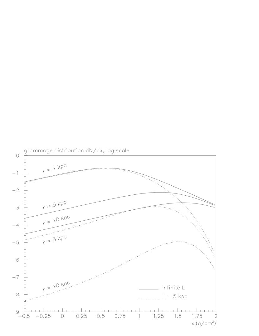
Figure 4: The path-length distribution ($x$ in g cm^-2) is shown for a point source and for different $r$. The two situations $L=5$ kpc and $L$ infinite are shown for comparison. The short grammages are depleted for remote sources, as the probability to travel a long distance without crossing the disc is small. This effect is all more pronounced that $L$ is small. The normalisation also decreases with $L$, which reflects the corresponding decrease of flux.

2.3.2 Impact on the chemical composition

The path-length distributions (11) are displayed in Figs. 3 and 4, for several propagation conditions, to emphasize the relative effect of escape, galactic wind and spallation. The effect of escape or wind is more important at higher grammages. This was expected as they correspond to longer paths. The effect of the convective wind is seen to be similar to that of escape, but quantitatively different at low grammages. To understand this, let us first consider diffusion in free space without wind. Several kinds of paths are responsible for low grammages: short paths, connecting us to nearby sources in the disk, and longer paths that wander in the halo without crossing the disk too much. It happens that the second kind is rather important, which explains why escape from a boundary at $z=\pm L$ (which kills the paths wandering too far in the halo) actually affects the low end of the grammage distribution. When wind is present, the short paths are more important, and the low grammages are less affected.

Even for a point source, the path-lengths are quite broadly distributed around the mean value, as can be seen in Figs. 3 and 4. As a result, the grammage distribution due to a set of discrete sources is smoothed to a great extent, and that it is very unlikely to have observable consequences on the composition of Cosmic Rays on Earth, except for very nearby sources (see below). To illustrate this point, we compare the grammage distributions and the B/C ratio from a smooth distribution to that obtained from a discrete sample representative of this distribution. The relative importance of the sources located at different distances in making the observed composition (e.g. the B/C ratio) was estimated and discussed in Taillet and Maurin (2003), and it was found that the nearby sources can be responsible for a substantial fraction of the flux of each species. The contribution of a point source located at a distance $r$ to the B and C flux, obtained from (11), is displayed as a function of $r$ in Fig. 11. More specifically, we divide the sources into the far ($r>L$), the intermediate ($0.1L<r<L$) and the nearby ($r<0.1L$), and Table 1 gives the fraction of flux coming from these regions, for different species.

	B	C	sub-Fe	Fe	$n_{B/C}$(kpc-2)
$0<r/L<0.1$	3 %	12 %	7 %	20 %	–
$0.1<r/L<1$	57 %	65 %	71 %	68 %	100
$1<r/L$	40 %	23 %	22 %	11 %	20

Table 1: The first four columns give, for the four species indicated (B, C, sub-Fe and Fe), the fraction of flux due to the three rings defined in the left column ($0<r/L<0.1$, $0.1<r/L<1$ and $1<r/L$), in the case of a homogeneous source distribution. The last column gives $n_{B/C}$, the surface number density of discrete sources (in kpc^-2), randomly distributed in these rings, beyond which the difference in flux with the continuous case is smaller than 1 %. There is no number given for the inner ring because there is no motivation to randomly draw the sources located very close to us, as these should be observed. The quantity $n_{B/C}$ was computed for $L=1$ kpc and should be divided by $L^{2}$ for other values. It does not depend on the value of $K$. The effect of the convective wind can be estimated by replacing $L$ by $L^{\star}\equiv K/V_{c}=r_{\rm w}/2$.

The grammage distribution from a ring delimited by $R_{\rm min}$ and $R_{\rm max}$ is given by

$${\cal G}(r,z=0,x) = \frac{1}{2\pi v\Sigma^{0}_{\rm ism}}\frac{2}{R_{\rm max}^{2}-R_{\rm min}^{2}}$$ (12)

$$\times \int_{0}^{\infty}dk\,\left\{R_{\rm max}J_{1}(kR_{\rm max})-R_{\rm min}J_{1}(kR_{\rm min})\right\}\,\exp\left(-\frac{x}{x(k)}\right)\;.$$ (13)

We randomly draw the position of sources inside each ring, with a given surface density of sources, we compute the corresponding flux, and the relative difference with the smooth case is computed. As expected, this difference gets smaller as the source density is increased, i.e. as the granularity of the source distribution is decreased. Table 1 gives $n_{B/C}$, the surface number density of sources in the disk (in kpc^-2) beyond which the difference in composition between the discrete and continuous case is less than 1 %. The secondaries are less sensitive to the discreteness of sources, as their sources (the primaries) do have a continuous distribution. These results do not depend on the value of $K$, as it is only sensitive to the relative importance of nearby and remote sources.

The results are presented as a function of $r/L$. If we now consider the disk defined by $r<1$ kpc, the resulting effect of granularity is quite insensitive to the value of $L$ (or $V_{c}$), as long as $L>1$ kpc (or $r_{w}>1$ kpc). This is because for $r<L$ (or $r<r_{w}$), the cut-off effect of escape (or wind) is always small. As expected, the effect of discreteness is smaller for the outer rings. The main effect is that when discrete sources are considered, the very nearby sources necessary to flatten the low end of the distribution are always lacking. Another way of phrasing this result is that shot noise is dominated by the nearby sources. The absence of nearby sources had been proposed by Lezniak and Webber (1979) to explain, in a different context, the depletion at low grammages that was thought to be observed, before Webber et al. (1998) proposed a settlement to this particular issue. The total path-length distribution is very close to an exponential, as expected for a homogeneous source distribution in an infinite disk (Jones, 1979).

Figure 5: The contributions to the path-length distribution (thick line) from continuous sources distributed in several rings (thin lines) are displayed for $L=5$ kpc. The path-length distribution from a set of 100 point sources drawn randomly in the central ring (inner 1 kpc) is also shown (dotted line). The effect of discreteness is most visible for low grammages. For the other rings, the difference between the continuous distribution and 200 discrete sources is of the order of a percent. The effect of galactic wind is very similar to that of $L$, replacing $L$ by $L^{\star}\equiv K/V_{c}=r_{\rm w}/2$.

The effect of the wind is very similar to that of escape. It has been remarked by Jones (1978) that to a given value of $V_{c}$ (in the case where the wind velocity is constant in each side of the halo) can be associated an effective escape height $L^{\star}=K/V_{c}=r_{\rm w}/2$, and we have explicitly checked that the previous results apply by replacing $L$ by $L^{\star}$.

2.4 Constant versus linear galactic wind

The previous results, as well as the results presented in our previous works, rely on the assumption of a constant wind presenting a discontinuity through the galactic disk. To probe the sensitivity of our results to this hypothesis, we consider another model in which the value of $V_{c}=V_{0}z$ varies linearly with $z$. This corresponds to the choice made e.g. in the widely used code galprop. The calculations are detailed in Appendix C, and the results will be used here without further justification. The path-length distribution reads

$$N(r,z,x)=\sum_{i}2hq_{i}J_{0}\left(\zeta_{i}\frac{r}{R}\right)\exp\left(-\frac{x}{x_{i}}\right)\Theta(x)$$

with

$$x_{i}=\frac{mv\Sigma^{0}_{\rm ism}L}{2K}\frac{\displaystyle\phi\left(\frac{3+a_{i}}{4},\frac{3}{2};\frac{V_{0}L^{2}}{2K}\right)}{\displaystyle\phi\left(\frac{1+a_{i}}{4},\frac{1}{2};\frac{V_{0}L^{2}}{2K}\right)}\;\;\;,\;\;\;a_{i}\equiv\frac{2K}{V_{0}}\frac{\zeta_{i}^{2}}{R^{2}}+2\;.$$

where $\phi$ is the confluent hypergeometric function, also denoted ${}_{1}F_{1}$ or $M$ in the literature. The resulting path-length distribution is shown in Fig. 6 for a linear and a constant (and discontinuous at $z=0$) wind. It appears that these two situations lead to very similar results, and one can establish a one-to-one correspondence between the parameters $V_{c}$ and $V_{0}$ of these models (see Fig. 7).

Figure 6: Path-length distributions for a linear (symbols, $V_{0}=0.018$ kpc Myr^-1 kpc^-1) and a constant galactic wind (line, $V_{c}=0.01$ kpc Myr^-1). It appears that the effect of a linear or constant wind are very similar. For each value of $V_{0}$, it is possible to find a value of $V_{c}$ yielding a grammage distribution which is very similar, with an accuracy better that one percent.

Figure 7: Correspondence between the values of $V_{c}$ for a constant wind ($x$ axis) and $V_{0}$ for a linear wind ($y$ axis) giving approximately the same path-length distributions, for two values of $L$.

It must be noted that the energy losses have not been considered here. Adiabatic losses are associated to the wind gradient, and their effect should be different for the two forms of the galactic wind: in the constant case, they are confined to the disk whereas in the linear case, they are present in the whole diffusive volume.

3 Time-dependent diffusion equation

3.1 Solutions

We now turn to the problem of discreteness in time. For that, we must solve the time-dependent diffusion problem for an instantaneous source. Diffusion occurs independently in the $z$ and $r$ directions. Neglecting the radial boundary, pure diffusion occurs in the radial direction and the density can be written as

$$N(r,z,t)=\frac{1}{4\pi Kt}e^{-r^{2}/4Kt}\,N(z,t)$$

where the function $N(z,t)$ satisfies a time dependent diffusion equation along $z$. It is convenient to introduce the quantities $k_{\rm s}=K/hv\sigma n_{\rm ism}$ and $k_{\rm w}=2K/V_{c}$, so that $N(z,t)$ is a solution of

$$\frac{\partial N}{\partial(Kt)}=\frac{\partial^{2}N}{\partial z^{2}}-2k_{\rm w}\,\mbox{sign}(z)\,\frac{\partial N}{\partial z}-2k_{\rm s}\delta(z)N\;.$$

For point-like and instantaneous sources, the radial distribution in the disk is given by (see Appendix A)

$$N(r,z=0,t)=\frac{1}{4\pi Kt}\exp\left(-\frac{r^{2}}{4Kt}\right)\sum_{n=1}^{\infty}c_{n}^{-1}e^{-(k_{n}^{2}+k_{\rm w}^{2})Kt}\sin^{2}\{k_{n}L\}\;.$$ (14)

where the discrete set of $k_{n}$ are the solutions of

$$k_{n}\,\mbox{cotan}(k_{n}L)=-k_{\rm s}-k_{\rm w}$$ (15)

and

$$c_{n}=L-\frac{\sin 2k_{n}L}{2k_{n}}=L+\frac{(\sin k_{n}L)^{2}}{k_{n}^{2}}\left(k_{\rm s}+k_{\rm w}\right)\;.$$

Though it is not immediately apparent in the expression (14), the spallations are taken into account, through the Eq. (15) determining the $k_{n}$. Moreover, this expression is more general than the form that is usually found in the literature, considering only the effects of escape, which is obtained by replacing the right-hand side of Eq. (15) by 0.

The result for a source that would accelerate particles for a long period of time would be obtained by integrating the above expression over the acceleration period. Finally, when energy losses are not considered, a whole energy spectrum is also simply accounted for by a linear superposition of delta-function sources.

3.2 Interpretation - Relative importance of nearby/recent sources

The expression (14) can be written as

$$N(r,z=0,t)=\frac{1}{(4\pi Kt)^{3/2}}\exp\left(-\frac{r^{2}}{4Kt}\right)g(t)\;,$$

where the function $g(t)$ gives the correction to the purely diffusive case and takes into account all the relevant physical effects. As such, it depends on the propagation parameters (spallation cross-section, galactic wind, halo height, diffusion coefficient). The importance of these effects depends on the position of the source in the $(r,t)$ plane. In particular, the old (large $t$) and remote (large $r$) sources are more affected by all these effects. For large values of $t$, $g(t)$ goes rapidly to zero, ensuring the convergence of the integral over time in Eq. (2). It also makes the function of $r$ obtained by this integration decreases faster that $1/r$, thus ensuring the convergence of the integral over $\vec{r}$.

This expression will be applied in a next study to the observed distribution of sources. For now, we want to illustrate the possible effect of discreteness in time. For that, we divide the sources into several decades in age, and we compute their contribution to the total spectrum. The energy spectrum of a primary species can be obtained by taking into account the energy dependence of $K$ in expression (14).

Figure 8: The contribution to the spectrum from different age classes is displayed for a uniform source distribution. In the more recent age class (0.001 Myr $<t<$ 0.01 Myr), the contribution from nearby sources ($r<1$ kpc) has been separated from the rest ($r>1$ kpc). The effect of time discreteness will be more important in this recent age class, which contains less sources.

The result is shown in Fig. 8, where the source distribution has been assumed to be uniform in the disk. If we denote by $\bar{r}$ the average distance from the sources to the Earth, the age $t$ gives the contribution at the energy $E$ for which $\bar{r}\sim\sqrt{K(E)t}$. The more recent sources dominate the high energy tail of the spectrum. This is where the effect of discreteness in time is expected to be the greatest, as the lower decades in age contain the smallest number of sources. For the more recent decade, the sources have been further split into nearby ($0.1$ kpc $<r<1$ kpc) and bulk ($r>1$ kpc). For a rate of 3 SN explosions by century in our Galaxy, there should be about 3 nearby sources in the more recent age decade. It is therefore probably important to know the actual position and age of these sources, and to correctly model propagation from these sources, e.g. from Eq. 14.

3.3 Reformulation of the steady-state model

The steady-state density results from the continuous superposition of solutions for instantaneous sources, and thus can be derived from the time-dependent solution discussed above:

$$N_{\rm stat}(r,z)=\int_{-\infty}^{0}N(r,z,t)\,dt\;.$$

The integration yields

$$N_{\rm stat}(r,z)=\frac{1}{K}\exp\left(-k_{\rm s}|z|\right)\sum_{n=1}^{\infty}c_{n}^{-1}K_{0}\left(r\sqrt{k_{n}^{2}+k_{\rm w}^{2}}\right)\sin(k_{n}L)\,\sin\left\{k_{n}(L-|z|)\right\}$$

where the Bessel function of the third kind $K_{0}$ has been introduced. This expression provides an alternative (but is exactly equivalent) to the usual Fourier Bessel expansion over $J_{0}$ functions. The functions $K_{0}$ over which the development is performed do not oscillate, inducing a faster convergence. It is thus particularly well suited for sources sharply localized in space, as point-like sources. We have checked that this expression is fully equivalent to the Fourier-Bessel expansion.

4 Summary and conclusion

The distribution of cosmic rays sources is not continuous. The granularity of the distribution has observable effects on the fluxes, spectra and composition, and thus should be considered when interpreting observed quantities. We have presented an analytical solution of the diffusion problem for an instantaneous point source, which takes this effect into account when the effects of escape through the boundaries $z=\pm L$, convective wind and spallation are considered. The next step is to apply this solution to the observed local distribution of cosmic ray sources.

Appendix A Time dependent solution of the diffusion equation

We consider diffusion in a cylindrically symmetric box, where both disk spallations and galactic wind have been taken into account. The convection velocity $\vec{V_{c}}$ lies in the vertical direction and drags the particles outside so that its value is given by $\mbox{sign}(z)\,V_{c}$ where a constant value for $V_{c}$ has been assumed. The diffusion equation reads, introducing the quantities $k_{\rm s}=hv\sigma n_{\rm ism}/K$ and $k_{\rm w}=V_{c}/2K$,

$${\displaystyle\frac{1}{K}\frac{\partial N}{\partial t}}=\left\{\frac{1}{r}{\displaystyle\frac{\partial}{\partial r}}\left(r{\displaystyle\frac{\partial N}{\partial r}}\right)+{\displaystyle\frac{\partial^{2}N}{\partial z^{2}}}\right\}-2k_{\rm w}\,\mbox{sign}(z)\,{\displaystyle\frac{\partial N}{\partial z}}-k_{\rm s}\delta(z)N\;\;.$$ (A1)

As boundaries in the radial direction $r$ play little role in our analysis, the galactic disk is modelled as an infinite flat disk in the $xOy$ plane. It is furthermore sandwiched by two confinement layers that extend to $z=\pm L$. The aim of this section is to derive the contribution of a source $S$ located at $\left\{x=0,y=0,z=0\right\}$ and exploding at time $t=0$ to the subsequent cosmic-ray density anywhere else in the Galaxy at location $P\,\left\{x,y,z\right\}$. The initial density reduces to the Dirac distribution

$$N(x,y,z,t=0)\equiv\delta(x)\,\delta(y)\,\delta(z)\;\;,$$ (A2)

and we would like to compute it at any time $t>0$. The radial diffusion is independent from diffusion along $z$, and is not affected by any of the processes other than diffusion. As a result, the solution can be factorized into

$$N(x,y,z,t)=\frac{1}{4\pi Kt}\,\exp\left\{-\frac{r^{2}}{4Kt}\right\}\,n(z,t)\;\;.$$ (A3)

where $n$ is a solution of

$$\frac{1}{K}\frac{\partial n}{\partial t}=\frac{\partial^{2}n}{\partial z^{2}}-k_{\rm w}\,\mbox{sign}(z)\,\frac{\partial n}{\partial z}-k_{\rm s}\delta(z)n\;\;,$$ (A4)

The trick is to factorize once again the time $t$ and the vertical $z$ behaviors so that $n\equiv f(z)\,g(t)$, which separates the diffusion equation into

$$g^{\prime}=-\alpha g\;\;\;\mbox{and}\;\;\;f^{\prime\prime}-2k_{\rm w}\,\mbox{sign}(z)\,f^{\prime}-k_{\rm s}\delta(z)f+\frac{\alpha}{K}f=0$$ (A5)

The resulting solution may appear contrived and exceptional. Actually an infinite set of such functions obtains that turns out to be a natural basis for the generic solutions to equation (A4). The time behavior amounts to the exponential decrease $g(t)=\exp\left(-\alpha t\right)$. The equation on $f$ can be solved for $z>0$ and $z<0$ with the appropriate boundary conditions $f(z=\pm L)=0$ as

$$f(z)=A\sinh\left\{k(L-|z|)\right\}\;\;\mbox{when}\;\;V_{c}^{2}-4K\alpha>0$$

$$f(z)=A\sin\left\{k(L-|z|)\right\}\;\;\mbox{when}\;\;V_{c}^{2}-4K\alpha<0$$ (A6)

with $k^{2}=\alpha/K-V_{c}^{2}/4K$. The first possibility does not fulfill the disk crossing condition (eq. A7 with hyperbolic functions). We therefore disregard it. We then insert (A6) into (A5). Derivation is to be understood in the sense of distributions, because of the singularity of $|z|$ in $z=0$. This yields

$$Kf^{\prime\prime}(z)=-\alpha f(z)-2KkA\delta(z)\cos kL$$

Inserting into (A5) gives the condition

$$2k\,\mbox{cotan}(kL)=-k_{\rm s}-k_{\rm w}$$ (A7)

The general solution reads

$$N(z,t)=\sum_{n=1}^{\infty}A_{n}e^{-\alpha_{n}t}\sin\left\{k_{n}(L-|z|)\right\}$$

The functions $\sin\{k_{n}(L-|z|)\}$ form an orthogonal set, and it is found that

$$\int_{-L}^{L}\sin\left\{k_{n}(L-|z|)\right\}\sin\left\{k_{n^{\prime}}(L-|z|)\right\}\,dz=\delta_{n{n^{\prime}}}c_{n}$$

with

$$c_{n}=L-\frac{\sin 2k_{n}L}{2k_{n}}$$ (A8)

The $A_{n}$ are found by imposing that for $t=0$, the distribution is a Dirac function,

$$\delta(z)=\sum_{n=1}^{\infty}A_{n}\sin\left\{k_{n}(L-|z|)\right\}$$

Multiplying by $\sin\{k_{m}(L-|z|)\}$ and integrating over $z$ yields

$$A_{m}=c_{m}^{-1}\sin k_{m}L$$

so that finally

$$N(z,t)=\sum_{n=1}^{\infty}c_{n}^{-1}e^{-\alpha_{n}t}\sin(k_{n}L)\,\sin\left\{k_{n}(L-|z|)\right\}$$ (A9)

and

$${\cal N}(r,z,t)=\frac{1}{4\pi Kt}\exp\left(-\frac{r^{2}}{4Kt}\right)\sum_{n=1}^{\infty}c_{n}^{-1}e^{-\alpha_{n}t}\sin(k_{n}L)\,\sin\left\{k_{n}(L-|z|)\right\}$$ (A10)

The radial distribution in the disk is given by

$${\cal N}(r,z=0,t)=\frac{1}{4\pi Kt}\exp\left(-\frac{r^{2}}{4Kt}\right)\sum_{n=1}^{\infty}c_{n}^{-1}e^{-k_{n}^{2}Kt}\sin^{2}(k_{n}L)$$ (A11)

Appendix B Path-length distribution for a non homogeneous spallative disk

This section details the derivation of expression (7), giving the grammage distribution in the case of an arbitrary radial distribution of spallative matter. The general method was sketched in Wallace (1981) to derive the cosmic ray density profile, and we present here a more general version which gives the grammage distribution.

We start from Eq. (3) for the steady-state case

$$0=K\left\{\frac{1}{r}\frac{\partial}{\partial r}\left(r{\cal G}(r,z,x)\right)+\frac{\partial^{2}{\cal G}(r,z,x)}{\partial z^{2}}\right\}+q(r)\delta(z)\delta(x)-\frac{\partial{\cal G}(r,z,x)}{\partial x}vm\Sigma^{0}_{\rm ism}f(r)\delta(z)$$

with $f(r)\equiv\Sigma_{\rm ism}(r)/\Sigma^{0}_{\rm ism}$ and $\Sigma^{0}_{\rm ism}=6.2\,10^{20}$ cm^-2 (Ferrière, 1998). We perform Fourier-Bessel transforms using the $J_{0}$ functions,

$${\cal G}(r,z,x)=\sum_{i=0}^{\infty}{\cal G}_{i}(z,x)J_{0}\left(\zeta_{i}\frac{r}{R}\right)\;\;\;\mbox{and}\;\;\;f(r){\cal G}(r,z=0,x)=\sum_{i=0}^{\infty}f_{i}(x)J_{0}\left(\zeta_{i}\frac{r}{R}\right)$$

with

$${\cal G}_{i}(z,x)=\frac{2}{J_{1}^{2}(\zeta_{i})}\int_{0}^{1}\rho J_{0}\left(\zeta_{i}\rho\right){\cal G}(\rho R,z,x)d\rho$$

$$f_{i}(x)=\frac{2}{J_{1}^{2}(\zeta_{i})}\int_{0}^{1}\rho J_{0}\left(\zeta_{i}\rho\right)f(\rho R){\cal G}(\rho R,z=0,x)=\sum_{j=0}^{\infty}\alpha_{ij}{\cal G}_{j}(0,x)$$

where we have introduced the matrix

$$\alpha_{ij}=\frac{2}{J_{1}^{2}(\zeta_{i})}\int_{0}^{1}\rho\,J_{0}(\zeta_{i}\rho)J_{0}(\zeta_{j}\rho)f(\rho r)\,d\rho$$

These expressions are reminiscent of those of Wallace (1981) that was dedicated to a perturbative resolution of the diffusion equation in the presence of an arbitrary matter distribution (with no description of the path-length distribution). The generalized diffusion equation reads

$$0=K\left\{\frac{\zeta_{i}^{2}}{R^{2}}{\cal G}_{i}(z,x)+\frac{\partial^{2}{\cal G}_{i}(z,x)}{\partial z^{2}}\right\}+q_{i}\delta(z)\delta(x)-\frac{\partial f_{i}(x)}{\partial x}vm\Sigma^{0}_{\rm ism}\delta(z)$$ (B1)

The solution for $z\neq 0$ satisfying $f(z=\pm L,x)=0$ is

$${\cal G}_{i}(z,x)={\cal G}_{i}(0,x)\frac{\sinh\left(\zeta_{i}(L-|z|)/R\right)}{\sinh\left(\zeta_{i}L/R\right)}$$

This expression is inserted back in the diffusion equation, taking care of the singularity of $|z|$ in 0 which yields

$$0={\cal G}_{i}(0,x)+\frac{q_{i}}{K}\frac{R}{2\zeta_{i}}\tanh\left(\frac{\zeta_{i}L}{R}\right)\delta(x)-\frac{vm\Sigma^{0}_{\rm ism}R}{2\zeta_{i}K}\tanh\left(\frac{\zeta_{i}L}{R}\right)\sum_{j=0}^{\infty}\alpha_{ij}\frac{\partial{\cal G}_{j}(0,x)}{\partial x}$$ (B2)

The solutions of this linear set of coupled first order differential equations are

$${\cal G}_{i}(0,x)=\sum_{j=0}^{\infty}a_{ij}e^{-x/x_{j}}\,\Theta(x)$$ (B3)

where the $x_{j}$ are the eigenvalues of the matrix

$$A_{ij}=\frac{vm\Sigma^{0}_{\rm ism}R}{2K\zeta_{i}}\tanh\left(\frac{\zeta_{i}L}{R}\right)\alpha_{ij}$$

Indeed, inserting expression (B3) in (B1), and using

$$\frac{\partial{\cal G}_{j}(0,x)}{\partial x}=-\sum_{k=0}^{\infty}\frac{a_{jk}}{x_{k}}e^{-x/x_{k}}\Theta(x)+\delta(x)\sum_{k=0}^{\infty}a_{jk}$$

we find an equation that can be separated in a regular part (factor of $\Theta(x)$) and a singular part (factor of $\delta(x)$). The former reads

$$\sum_{j=0}^{\infty}a_{ij}e^{-x/x_{j}}-\frac{vm\Sigma^{0}_{\rm ism}R}{2\zeta_{i}K}\tanh\left(\frac{\zeta_{i}L}{R}\right)\sum_{k=0}^{\infty}\alpha_{ik}\sum_{j=0}^{\infty}\frac{a_{kj}}{x_{j}}e^{-x/x_{j}}=0$$

In order for each coefficient of $e^{-x/x_{j}}$ to be zero, one must have

$$a_{ij}-\frac{vm\Sigma^{0}_{\rm ism}R}{2\zeta_{i}Kx_{j}}\tanh\left(\frac{\zeta_{i}L}{R}\right)\sum_{k=0}^{\infty}\alpha_{ik}a_{kj}=0$$ (B4)

so that

$$\det\left[x_{j}\delta_{ik}-\frac{vm\Sigma^{0}_{\rm ism}R}{2\zeta_{i}K}\tanh\left(\frac{\zeta_{i}L}{R}\right)\alpha_{ik}\right]=0$$ (B5)

This shows that the $x_{i}$ are eigenvalues of $A_{ij}$. This equation alone is then not enough to compute the $a_{ij}$. An extra relation is provided by the singular part

$$-\frac{vm\Sigma^{0}_{\rm ism}R}{2\zeta_{i}K}\tanh\left(\frac{\zeta_{i}L}{R}\right)\sum_{j=0}^{\infty}\alpha_{ij}\sum_{k=0}^{\infty}a_{jk}=-\frac{q_{i}}{K}\frac{R}{2\zeta_{i}}\tanh\left(\frac{\zeta_{i}L}{R}\right)$$

which gives

$$\sum_{k=0}^{\infty}\sum_{j=0}^{\infty}\alpha_{ij}a_{jk}=\frac{q_{i}}{vm\Sigma^{0}_{\rm ism}}$$ (B6)

The coefficients $a_{ij}$ are completely set by Eqs (B4) and (B6).

When the galactic wind is taken into account, a more tedious derivation shows that Eq. (B2) should be replaced by

$$0={\cal G}_{i}(0,x)+\frac{q_{i}}{2K}\left[\frac{1}{r_{\rm w}}+S_{i}\coth\left(\frac{\zeta_{i}L}{R}\right)\right]^{-1}\delta(x)-\frac{vm\Sigma^{0}_{\rm ism}}{2K}\left[\frac{1}{r_{\rm w}}+S_{i}\coth\left(\frac{\zeta_{i}L}{R}\right)\right]^{-1}\sum_{j=0}^{\infty}\alpha_{ij}\frac{\partial{\cal G}_{j}(0,x)}{\partial x}$$ (B7)

so that the same results apply, provided that one makes the substitution

$$\frac{R}{2\zeta_{i}}\tanh\left(\frac{\zeta_{i}L}{R}\right)\rightarrow\left(\frac{1}{r_{\rm w}}+S_{i}\coth\left(\frac{S_{i}L}{2}\right)\right)^{-1}\;\;\;\mbox{and}\;\;\;S_{i}=2\left(\frac{1}{r_{\rm w}^{2}}+\frac{\zeta_{i}^{2}}{R^{2}}\right)^{1/2}$$

Appendix C Linear galactic wind in the steady-state cylindrical disk-halo model

Resolution of the diffusion equation for a stable primary

We write $V_{c}(z)=V_{0}z$, and the steady-state diffusion equation reads (see also Bloemen et al., 1993)

$$0=\frac{K}{r}\frac{\partial}{\partial r}\left\{r\frac{\partial N}{\partial r}\right\}-\frac{\partial N}{\partial z}\left\{-K\frac{\partial N}{\partial z}+V_{0}zN\right\}-\sigma\Sigma v\delta(z)N+2hq\delta(z)$$

Developing over Bessel functions,

$$-\frac{2hq_{i}}{K}\delta(z)=-\frac{\zeta_{i}^{2}}{R^{2}}\,N_{i}+\frac{\partial^{2}N_{i}}{\partial z^{2}}-\frac{V_{0}z}{K}\,\frac{\partial N_{i}}{\partial z}-\frac{V_{0}}{K}N_{i}-\frac{\sigma\Sigma v}{K}\delta(z)N_{i}$$

It is convenient to rewrite this equation in a hermitic differential form, to ensure that the solutions form an orthogonal set of functions (see e.g. Morse & Feshbach 1953). We introduce $n_{i}=N_{i}\exp(-k^{2}z^{2}/2)$, $\beta=V_{0}/4K$ and $y=kz$ with $k=\sqrt{V_{0}/2K}$, which yields, in the halo

$${n_{i}}^{\prime\prime}-n_{i}\left(a_{i}+y^{2}\right)=0$$

where

$$a_{i}\equiv\frac{2K}{V_{0}}\frac{\zeta_{i}^{2}}{R^{2}}+2$$

The solutions are of the form, taking into account the condition $n_{i}(z=\pm L)=0$,

$$n_{i}=B_{i}\,e^{-k^{2}z^{2}/2}\left\{\phi\left(\frac{1+a_{i}}{4},\frac{1}{2};k^{2}z^{2}\right)-\frac{z}{L}\frac{\displaystyle\phi\left(\frac{1+a_{i}}{4},\frac{1}{2};k^{2}L^{2}\right)}{\displaystyle\phi\left(\frac{3+a_{i}}{4},\frac{3}{2};k^{2}L^{2}\right)}\,\phi\left(\frac{3+a_{i}}{4},\frac{3}{2};k^{2}z^{2}\right)\right\}$$

where $\phi$ is the confluent hypergeometric function, also noted ${}_{1}F_{1}$. The value of $B_{i}$ is found by integrating the diffusion equation through the disk, so that

$$2\left.\frac{dn_{i}}{dz}\right|_{z=0}=\frac{\sigma\Sigma^{0}_{\rm ism}v}{K}n_{i}(0)-\frac{2hq_{i}}{K}$$

This gives $B_{i}=2hq_{i}/A_{i}$ with

$$A_{i}=\frac{2K}{L}\frac{\displaystyle\phi\left(\frac{1+a_{i}}{4},\frac{1}{2};k^{2}L^{2}\right)}{\displaystyle\phi\left(\frac{3+a_{i}}{4},\frac{3}{2};k^{2}L^{2}\right)}+v\sigma\Sigma^{0}_{\rm ism}$$ (C1)

The final solution is thus obtained as

$$N(r,z)=\sum_{i}\frac{2hq_{i}}{A_{i}}J_{0}\left(\zeta_{i}\frac{r}{R}\right)\left\{\phi\left(\frac{1+a_{i}}{4},\frac{1}{2};k^{2}z^{2}\right)-\frac{z}{L}\frac{\displaystyle\phi\left(\frac{1+a_{i}}{4},\frac{1}{2};k^{2}L^{2}\right)}{\displaystyle\phi\left(\frac{3+a_{i}}{4},\frac{3}{2};k^{2}L^{2}\right)}\,\phi\left(\frac{3+a_{i}}{4},\frac{3}{2};k^{2}z^{2}\right)\right\}$$ (C2)

The density in the disk is thus given by

$$N(r,z=0)=\sum_{i}\frac{2hq_{i}}{A_{i}}J_{0}\left(\zeta_{i}\frac{r}{R}\right)$$ (C3)

It can be shown that this expression reduces to the usual expressions in the case of a vanishing wind.

The path-length distribution

The dependence in $\sigma$ is very simple and the path-length distribution is obtained by inverse Laplace transform as

$$N(r,z,x)=\sum_{i}2hq_{i}J_{0}\left(\zeta_{i}\frac{r}{R}\right)\exp\left(-\frac{x}{x_{i}}\right)\Theta(x)$$

with

$$x_{i}=\frac{mv\Sigma L}{2K}\frac{\displaystyle\phi\left(\frac{5}{4}+\frac{K}{2V_{0}}\frac{\zeta_{i}^{2}}{R^{2}},\;\frac{3}{2};\;\frac{V_{0}L^{2}}{2K}\right)}{\displaystyle\phi\left(\frac{3}{4}+\frac{K}{2V_{0}}\frac{\zeta_{i}^{2}}{R^{2}},\;\frac{1}{2};\;\frac{V_{0}L^{2}}{2K}\right)}$$

Appendix D Remark about the time evolution of the mean grammage

The mean grammage of the CR emitted by a single source can be expressed from the distribution ${\cal G}(\vec{r},x,t)$ as

$$\bar{X}(t)\equiv\frac{\displaystyle\int\!\!\!\int\!\!\!\int d^{3}\vec{r}\int_{0}^{\infty}dx\,x\,{\cal G}(\vec{r},x,t)}{\displaystyle\int\!\!\!\int\!\!\!\int d^{3}\vec{r}\int_{0}^{\infty}dx\,{\cal G}(\vec{r},x,t)}$$ (D1)

In this expression, the averaging process is understood to be performed over the whole spatial distribution of cosmic rays. The time derivative of this expression yields

$$\frac{d\bar{X}}{dt}=\frac{\displaystyle\int\!\!\!\int\!\!\!\int d^{3}\vec{r}\int_{0}^{\infty}dx\,x\,\partial{\cal G}(\vec{r},x,t)/\partial t}{\displaystyle\int\!\!\!\int\!\!\!\int d^{3}\vec{r}\int_{0}^{\infty}dx\,{\cal G}(\vec{r},x,t)}-\bar{X}\;\frac{\displaystyle\int\!\!\!\int\!\!\!\int d^{3}\vec{r}\int_{0}^{\infty}dx\,\partial{\cal G}(\vec{r},x,t)/\partial t}{\displaystyle\int\!\!\!\int\!\!\!\int d^{3}\vec{r}\int_{0}^{\infty}dx\,{\cal G}(\vec{r},x,t)}$$ (D2)

The denominator is simply $N(t)$, the total number of CR in the diffusive volume. Using the fact that

$$\frac{\partial{\cal G}}{\partial t}=-\bar{m}\beta cn(\vec{r})$$

where $n(\vec{r})$ is the interstellar gas density and integrating the first term by parts, we finally find,

$$\frac{d\bar{X}}{dt}=\bar{m}\beta c\,n_{sn}(t)-\bar{X}(t)\,\frac{1}{N}\frac{dN}{dt}$$ (D3)

where $n_{sn}(t)$ is defined as in (8). The last term is missing in Eq. 4.3 of Higdon and Lingenfelter (2003). This term is positive and represents the change in grammage due to the escape of a fraction of cosmic rays between times $t$ and $t+dt$.

As stressed in the text, a quantity which has a greater physical importance to us is the mean grammage of the CR that reach the Earth at time $t$, i.e.

$$\bar{x}(\vec{r},t)=\frac{\displaystyle\int_{0}^{\infty}dx\,x\,{\cal G}(\vec{r},x,t)}{\displaystyle\int_{0}^{\infty}dx\,{\cal G}(\vec{r},x,t)}$$ (D4)

Following the same procedure as above, its time evolution is given by

$$\frac{\partial\bar{x}(\vec{r},t)}{\partial t}=\bar{m}\beta c\,n(\vec{r})-\bar{x}(\vec{r},t)\,\frac{\partial}{\partial t}\left\{\ln w(\vec{r},t)\right\}$$ (D5)

where the definition of $w(\vec{r},t)$ is given in (10).

References

- Aharonian et al. (1995) Aharonian, F. A., Atoyan , A. M., Völk, H. J., 1995, A&A, 294, L41
- Benítez et al. (2002) Benítez, N., Maíz-Apellániz, J. and Canelles, M., 2002, Physical Review Letters, 88, 81101
- Bloemen et al. (1993) Bloemen, J. B. G. M., Dogiel, V. A., Dorman, V. L. and Ptuskin, V. S., 1993, A&A, 267, 372
- Coswik and Lee (1979) Cowsik, R. and Lee, M. A., 1979, ApJ, 228, 297
- Donato et al. (2002) Donato, F., Maurin, D., Taillet, R., 2002, A&A, 381, 539
- Dorman et al. (1985) Dorman, L. I., Ghosh, A. and Ptuskin, V. S., 1985, Ap&SS, 109, 87
- Erlykin and Wolfendale (2001a) Erlykin, A. D. and Wolfendale, A. W., 2001a, J.Physics G: Nucl. Part. Phys., 27, 941
- Erlykin and Wolfendale (2001b) Erlykin, A. D. and Wolfendale, A. W., 2001b, J.Physics G: Nucl. Part. Phys., 27, 959
- Ferrière (1998) Ferrière, K., 1998, ApJ, 497, 759
- Fields and Ellis (1999) Fields, B. D., Ellis, J., 1999, New Astronomy, 4, 419
- Forman and Schaeffer (1979) Forman, M. A. and Schaeffer, O. A., 1979, Reviews of Geophysics and Space Physics, 17, 552
- Freedman et al. (1980) Freedman, I., Giler, M., Kearsey, S. and Osborne, J. L., 1980, A&A, 82, 110
- Higdon and Lingenfelter (2003) Higdon, J. C, and Lingenfelter, R. E., 2003, ApJ, 582, 330
- Jones (1978) Jones, F. C., 1978, ApJ, 222,1097
- Jones (1979) Jones, F. C., 1979, ApJ, 229,747
- Johnson (1994) Johnson, 1994, Astroparticle Physics, 2, 257
- Knie et al. (1999) Knie, K., Korschinek, G., Faestermann, T., Wallner, C., Scholten, J., Hillebrandt, W., 1999, Physical Review Letters, 83, 18
- Lerche and Schlickeiser (1982) Lerche, I. and Schlickeiser, R., 1982, A&A, 116, 10
- Lezniak (1979) Lezniak, J. A., 1979, Ap&SS, 63, 279
- Lezniak and Webber (1979) Lezniak, J. A., and Webber, W. R., 1979, Ap&SS, 63, 35
- Margolis (1986) Margolis, S. H., 1986, ApJ, 300, 20
- Maurin et al. (2001) Maurin, D., Donato D., Taillet, R. and Salati, P., 2001, ApJ, 555, 585
- Morse & Feshbach (1953) Morse, P.M., Feshbach, H., Methods of Theoretical Physics (McGraw Hill, New York, 1953)
- Owens (1976) Owens, A. J., 1976, Ap&SS, 44, 35
- Ptuskin and Soutoul (1998) Ptuskin, V.S., Soutoul, A., 1998, A&A, 337, 859
- Ramadurai (1993) Ramadurai, 1993, Bull. Astr. Soc. India, 21, 391
- Shaviv (2002) Shaviv, N. J., 2002, Physical Review Letters, 89, 51102
- Stephens and Streitmatter (1998) Stephens, S. A. and Streitmatter, R. E., 1998, ApJ, 505, 266
- Taillet and Maurin (2003) Taillet, R., and Maurin, D., 2003, A&A, 402, 971
- Wallace (1981) Wallace, J. M., 1981, ApJ, 245, 753
- Webber et al. (1998) Webber, W. R., et al., 1998, ApJ, 508, 940