11email: girardi,mardiros,mezzetti,rigoni@ts.astro.it 22institutetext: Laboratoire d’Astrophysique de Marseille, Marseille, France
22email: marinoni@astrsp-mrs.fr
Galaxies in group and field environments:
a comparison of
optical–NIR luminosities and colors
We compare properties of galaxies in loose groups with those in field environment by analyzing the Nearby Optical Galaxy (NOG) catalog of galaxy systems. We consider as group galaxies, objects belonging to systems with at least five members identified by means of the “friends of friends method”, and, as field galaxies, all galaxies with no companions. We analyze both a magnitude–limited sample of 959 and 2035 galaxies (groups vs. field galaxies, respectively, B mag, and km s) and a volume–limited sample ( mag, km s369 group and 548 field galaxies). For all these galaxies, blue corrected magnitudes and morphological types are available. The cross-correlation of NOG with the 2MASS second release allow us to assign K magnitudes and obtain B–K colors for about half of the galaxies in our samples. We analyze luminosity and color segregation–effects in relation with the morphological segregation. For both B and K bands, we find that group galaxies are, on average, more luminous than field galaxies and this effect is not entirely a consequence of the morphological segregation. After taking into account the morphological segregation, the luminosity difference between group and field galaxies is about . When considering only very early–type galaxies (T) the difference is larger than . We also find that group galaxies are redder than field galaxies, (B–K) mag. However, after taking into account the morphological segregation, we find a smaller B–K difference, poorly significant (only at the c.l. of ). We discuss our results considering that the analyzed groups define a very low density environment (projected mean density h2 Mpc-2 galaxies).
Key Words.:
Galaxies: clusters: general – Galaxies: fundamental parameters – Galaxies: evolution – Cosmology: observations1 Introduction
In spite of the variety and number of devoted studies, we are still far from understanding how much of galaxy evolution is a reflection of local physics on galactic scales, possibly in the context of biased galaxy formation, and how much of it is due to environmental effects intrinsically connected to the parent galaxy-system.
Most of past studies concerning the effects of the external environment on galaxy evolution focused on central regions of galaxy clusters and consistently showed that early–type galaxies (or very luminous ones) inhabit preferentially cluster cores (e.g., Oemler oem74 (1974); Dressler dre80 (1980); Biviano et al. biv92 (1992); Dressler et al. dre97 (1997); Biviano et al. biv02 (2002)). More recent studies aim to analyze environmental effects as a function of radius out to larger and larger distances from the cluster center. These analyses probe the radial gradient in photometric and spectroscopic properties out to or just beyond the virial radius: the emerging picture is that galaxy star formation rate (SFR) is suppressed via via galaxies are accreted onto clusters (e.g., Abraham et al. abr96 (1996); Balogh et al. bal97 (1997); Pimbblet et al. pim02 (2002)). Very recent analyses based on the 2dF Galaxy Redshift Survey and on the Sloan Digital Sky Survey show that the distribution of SFRs of cluster galaxies begins to change, compared with the field population, at a clustercentric radius of 3-4 virial radii (Lewis et al. lew02 (2002); Gómez et al. gom03 (2003)). Moreover, the SFR of galaxies is strongly correlated with the local projected galaxy–density down to a characteristic threshold (Lewis et al. lew02 (2002); Gómez et al. gom03 (2003)). These environmental effects on the SFR are analogous to those on the galaxy morphology, known as the morphology-radius and morphology-density relations (e.g., Oemler oem74 (1974); Dressler dre80 (1980); Postman & Geller pos84 (1984); Whitmore et al. whi93 (1993)). Since SFR is lower in early–type galaxies (e.g., Kennicutt ken83 (1983); Jansen et al. jan00 (2000)), which inhabit preferentially cluster cores and high density regions, it is not clear whether the two effects are completely independent. First attempts suggest that morphology segregation alone is unlikely to explain the SFR effect (Balogh et al. bal98 (1998); Lewis et al. lew02 (2002); Pimbblet et al. pim02 (2002); Gómez et al. gom03 (2003) ).
Both traditional and more recent approaches, concerning morphologies and SFRs, respectively, consistently show that environmental influences on galaxy properties are not restricted to cluster cores, but are effective in groups, which could be the relevant sites of galaxy evolution (e.g., Balogh & Bower bal03 (2003)). Although the study of the group environment is a much more difficult task than the study of cluster environment, there are now robust observational evidences confirming that group galaxies of different morphological type – color – spectral type are spatially segregated (e.g., Ozernoy & Reinhard oze76 (1976); Postman & Geller pos84 (1984); Mahdavi et al. mah99 (1999); Tran et al. tra01 (2001); Carlberg et al. car01 (2001); Domínguez et al. dom02 (2002)). Luminosity segregation in groups is a more controversial issue (e.g., Ozernoy & Reinhard oze76 (1976); Giuricin et al. giu82 (1982); Mezzetti et al. mez85 (1985); Magtesyan & Movsesyan mag95 (1995)). Analyzing loose groups identified in the Nearby Optical Galaxy (NOG) sample by Giuricin et al. (giu01 (2001)), Girardi et al. (Girardi et al. gir03 (2003)) have found evidence of morphology and B–band luminosity segregation of galaxies both in space and in velocity, in qualitative agreement with a continuum of segregation properties of galaxy enbedded in systems, from low-mass groups to massive clusters.
The aim of this paper is to study the environmental dependence of galaxy properties, luminosities and colors, in very low density environments comparing loose groups and field in the NOG catalog. In particular, we use the large amount of morphological information available for nearby galaxies to disentangle and discriminate in a robust way luminosity and color segregation–effects from morphological segregation.
The outline of this paper is as follows. We describe the data sample and magnitude data in Sects. 2 and 3, respectively. We devote Sect. 4 to the analysis of luminosity and morphology segregation–effects, and Sect. 5 to color segregation. We discuss and summarize our results in Sects. 6 and 7, respectively.
Unless otherwise stated, we give errors at the 68% confidence level (hereafter c.l.).
A Hubble constant of 100 km sMpc-1 is used throughout.
2 Group and field samples
We analyze the NOG catalog (Giuricin et al. giu00 (2000)). NOG is a magnitude–limited catalog (corrected total blue apparent magnitude B), with an upper distance limit ( km s-1), which contains optical galaxies, basically extracted from the Lyon–Meudon Extragalactic Database (LEDA; Paturel et al. pat97 (1997). NOG covers about of the sky , and is quasi-complete in redshift (). Almost all NOG galaxies () have a morphological classification as taken from LEDA, and parameterized by (the morphological–type code system of RC3 catalog – de Vaucouleurs et al. dev91 (1991)) with one decimal figure.
Hereafter we consider only the galaxies with the full information available: i) galaxy position; ii) radial velocity , where is the heliocentric redshift in the LG rest frame (according to Yahil et al. yah77 (1977)); iii) corrected total blue magnitude; iv) morphology.
Group galaxies were identified by Giuricin et al. (giu00 (2000)) using the “friends–of–friends” method. In particular, by applying two different variants of the percolation method, they obtained two comparable catalogs of galaxy systems. Here we use the P2 catalog obtained by allowing both the distance and the velocity link parameters to scale with distance (Huchra & Geller huc82 (1982)); even if new 3D cluster finding algorithms have been recently proposed (e.g., Marinoni et al. mar02 (2002)) this is the most frequently used method of group identification for low redshift galaxies.
In order to obtain the best-quality group sample in our analysis we remove: i) all groups identified as known clusters (see Table 7 of Giuricin et al. giu00 (2000)); ii) all very poor groups with member galaxies. We remove clusters following our aim to study low density environments. Moreover, the clusters contained in the NOG catalog are very few (only ten at km s), not particularly rich (Abell richness ), and poorly sampled (10.5 is the median number of members). Thus NOG clusters are not a very representative sample of rich clusters to be useful in a comparison with group results. As for very poor groups, the efficiency of the percolation algorithm has been repeatedly checked, showing that an appreciable fraction of the poorer groups, those with members, might be false (i.e. represent unbound density fluctuations), whereas richer groups almost always correspond to real systems (e.g., Ramella et al. ram89 (1989); Ramella et al. ram95 (1995); Mahdavi et al. mah97 (1997); Nolthenius et al. nol97 (1997); Diaferio et al. dia99 (1999)). The dilution effect of a significant number of spurious groups in our analysis would hide or weaken any possible difference between groups and field. For instance, this dilution effect is suggested to explain some differences between groups with and with as concerning the segregation properties of member galaxies (Girardi et al. gir03 (2003), Sect. 4.3). In view of this possible bias we prefer to remove groups from our sample.
We consider as field galaxies, all the NOG galaxies left unbound, i.e. not belonging to any group or binary system.
Finally, we remove from our analysis all field galaxies with km sand groups with km s, where the mean group velocity is computed by using the biweight estimator (Beers et al. bee90 (1990)). In fact, where the recession velocity is not dominant on its random component, it is no longer a reliable indication of the distance. We apply such a conservative limit since our analysis requires accurate absolute magnitudes. In particular, the value of km sis suggested by the analysis of the velocity field in the local Universe where the effect of peculiar velocities is higher for km s(Marinoni et al. mar98 (1998)). Moreover, thank to our lower distance limit, all galaxies belonging to the main clumps and clouds of the Virgo cluster are rejected, too (see Binggeli et al. bing87 (1987); Binggeli et al. bin93 (1993); and Table 7 of Giuricin et al. giu00 (2000)).
Our final group sample contains 120 loose groups for a total of 959 galaxies (hereafter GROUP sample). The field sample contains 2035 galaxies (FIELD sample). Table 1 lists the median values for group main properties: number of members, , and redshift, . We also give the median values – with corresponding confidence intervals – and lower and upper quartiles of the distributions for: group size, , which is the (projected) distance of the most distant galaxy from the (biweight) group center; LOS velocity dispersion, , and virial mass, , computed following Girardi & Giuricin (gir00 (2000); see also Girardi et al. gir03 (2003)). The confidence intervals are computed following the procedure111 For the median of an ordered distribution of values the confidence intervals and , corresponding to a probability , can be obtained from . described by Kendall & Stuart (ken79 (1979), eq. 32.23) and first proposed by Thompson (tho36 (1936)).
| Mpc | km s | ||||||||
| Median | Lower, Upper | Median | Lower, Upper | Median | Lower, Upper | ||||
| 120 | 959 | 6 | 0.013 | 0.54, 0.90 | 119, 260 | 0.7, 5.2 | |||
Moreover, we also extract from the above magnitude–limited sample a volume–limited subsample, which by definition contain objects that are luminous enough to be included in the sample when placed at the cutoff distance. We define the volume–limited samples of group and field galaxies with depth of 4000 km sby considering only galaxies with blue corrected absolute–magnitude (hereafter VLGROUP and VLFIELD samples, respectively). The limit of 4000 km sis again suggested by the analysis of Marinoni et al. (mar98 (1998)), since the discrepancy between different peculiar velocity models derived using independent techniques is more pronounced for km s. The VLGROUP and VLFIELD (km s) samples contain 369 and 548 galaxies, respectively.
As for the comparison of GROUP vs. FIELD samples we have to check for possible biases connected with depth since these samples are extracted from an (apparent-) magnitude–limited sample (see Sect. 4.2, too). Fig. 1 shows the comparison of radial velocity distributions for field and group galaxies. Small differences are shown, probably due to very local differences in the clustering properties of large scale structure. Analyzing the corresponding cumulative distributions we find a difference at the 99.99% c.l., according to the Kolmogorov–Smirnov test (hereafter KS-test; e.g., Ledermann led82 (1982)). To avoid possible observational biases we construct a simulated sample of field galaxies which mimics the velocity distribution of group galaxies. We use the inverse transformation method for generating a random deviate from a known probability distribution as outlined in, e.g., Press et al. (pre92 (1992)). In practice, given the (normalized) distribution of velocities of group galaxies (in the range 0-6000 km s), , and the cumulative distribution, , we choose an uniform random : its corresponding is the desired deviate and we assign to the simulated field a galaxy of the real field very close to that velocity , i.e. one galaxy randomly selected in a range of km s. In this way we assign to the simulated field ten thousands of galaxies, of which are those with km s. As expected, there is no significant difference between the velocity distribution of simulated–field galaxies and that of group galaxies (see Fig. 1). Although general results are very similar (see Sect. 4.2), hereafter we consider the simulated field, S-FIELD, in any comparison with GROUP sample, after properly rescaling the number of simulated objects to that of real–field galaxies when statistical confidence levels are derived.
Note that in the above resampling we have used velocities of individual group galaxies rather than luminosity distances, the latter being based on mean velocities of the corresponding parent group. Our choice is due to the requirement of using a variable with a smooth, well-behaved probability distribution. In fact, the probability distribution of luminosity distances for group galaxies shows many peaks, which are higher for groups with a larger number of members. From the physical point of view, we use the KS-test to verify that the cumulative distribution of individual velocities of group galaxies does not significantly differ from that obtained substituting individual velocities with mean velocities. Thus any possible effect due to the chosen variable should be negligible.

.
3 Galaxy magnitudes and colors
NOG total, corrected B–band magnitudes come from LEDA compilation, which collects and homogenize data of several catalogs. They have been converted to the standard systems of the RC3 catalog (de Vaucouleurs et al. dev91 (1991)) and have been corrected for Galactic extinction, internal extinction, and –dimming (see Paturel et al. pat97 (1997) for more details).
We take Ks-band survey magnitudes, K20, from the extended catalog of the official 2MASS second release. To assign the counterpart of each galaxy in our sample we choose the closest 2MASS object within a search radius of 0.3 arcmin. We use this search radius to enclose also very nearby, with large angular size, galaxies. The typical angular separation between a NOG galaxy and its counterpart is much smaller (-5 arcsecs). We find counterparts for 3263 of 7076 galaxies of the whole NOG catalog. Out of these 3263 2MASS objects, the possible contamination of non-galaxy objects is quite small: only 56 objects have parameters which indicate a possible artifact or contaminated and/or confused source, i.e. , , (see Jarrett et al. jar00 (2000), Cole et al. col01 (2001)).
The fraction of matched galaxies corresponds to the incomplete sky coverage in the 2MASS 2nd release ( of the sky). Moreover, the B-magnitude distribution of matched 2MASS-NOG galaxies is not different from that of all NOG galaxies suggesting that 2MASS-NOG galaxies form an unbiased subsample of the whole NOG catalog (see Fig. 2).

As for our specific samples, we obtain K20 magnitude for 440 and 936 galaxies in GROUP and FIELD samples, respectively (167 and 240 galaxies in VLGROUP and VLFIELD, respectively).
To obtain total corrected K magnitudes we consider the offset of 0.2 mag between isophotal and total magnitudes (see Kochanek et al. koc01 (2001)) and we correct for Galactic extinction, internal extinction and –dimming:
| (1) |
We correct for Galactic extinction, E(B-V)], using the color excess E(B-V) recovered by the extinction maps of Schlegel et al. (sch98 (1998)) and an extinction coefficient of (Cardelli et al. car89 (1989)). For the term of internal extinction we assume Ei(B–V), where the internal B–band absorption of galaxies is for and for according to the mean values suggested by RC3 for different morphological types. Finally, we apply the Ks-band –correction of log, independent of galaxy type and valid for (based on the Worthey wor94 (1994) models, see Kochanek et al. koc01 (2001)).
We convert B– and K–band magnitudes to absolute magnitudes and by using the luminosity distance recovered from redshift . For group galaxies we use the of the parent group.
4 Luminosity and morphology environmental effects
4.1 Analysis and results
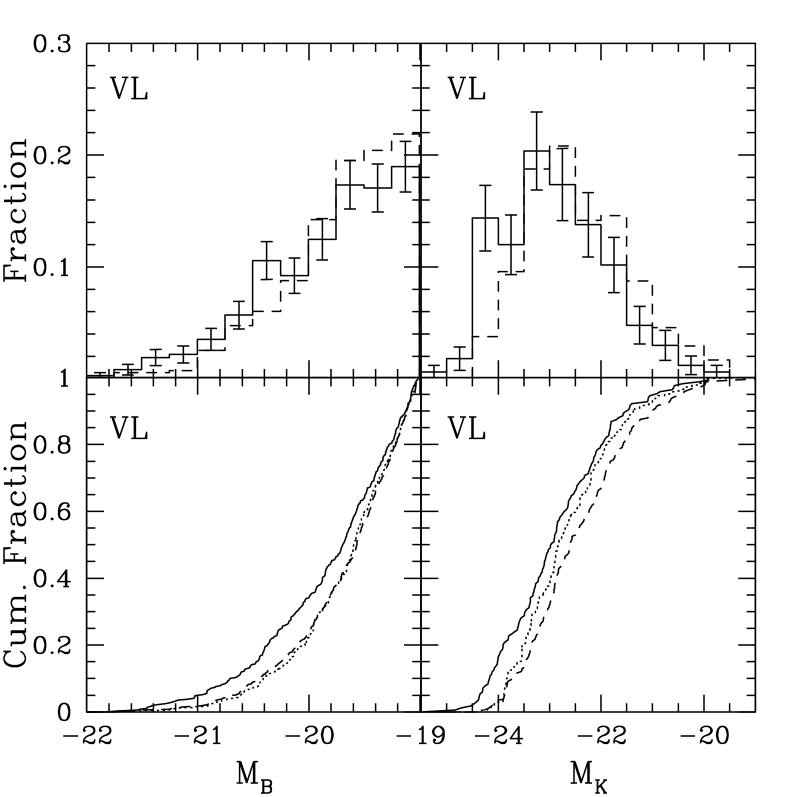
Figs. 3 and 4 show that group galaxies are more luminous in both B and K bands than field galaxies. To compute the significance of this difference, we compare the cumulative distributions of B magnitudes for GROUP and S-FIELD (VLGROUP and VLFIELD): they are different at the () according to the KS-test; the same result is found for K magnitudes.


The morphological distributions in group and field environments are different at the c.l. (according to the KS-test). In fact, the fraction of early galaxies in groups is larger than in the field (see Fig. 5). In particular, we compute the relative proportion of E+S0 (), S0+Searly (), Smiddle (), and Slate+I () obtaining (18:16:35:31) and (8:8:35:49) for GROUP and FIELD environments, respectively. The morphological–type distribution of S-FIELD galaxies is not different from that of FIELD.
To disentangle luminosity and morphological segregation–effects we consider mean luminosity values as a function of morphological types, see Figs. 6 and 7 (top panels). The difference is better outlined in the corresponding bottom panels where is shown: under the same morphological type, group galaxies are more luminous than the respective field galaxies. According to the -test, the null hypothesis is rejected at the () when comparing the GROUP and S-FIELD samples (VLGROUP and VLFIELD). As for K magnitudes, the null hypothesis is rejected at the () when comparing the GROUP and S-FIELD samples (VLGROUP and VLFIELD).


We prefer to avoid the arbitrary binning choice intrinsically connected to the use of the -test. Consequently we apply an alternative statistical method. We construct a simulated field (of 10000 galaxies) in order to mimic the morphological distribution of group galaxies and we do this by using the same technique outlined in Sect. 2. That is, after having selected a random deviate from the whole morphological–type distribution of GROUP (VLGROUP) galaxies, we assign to the simulated field a galaxy of the S-FIELD (VLFIELD) very close to that , i.e. one galaxy randomly selected in a range of . In this way we construct a simulated ST-S-FIELD (ST-VLFIELD) sample which has a -distribution similar to that of the GROUP (VLGROUP) sample. Figs. 3 and 4 (bottom panels) show the cumulative magnitude distribution of this simulated field for the magnitude– and volume–limited samples, respectively. According to the KS-test, we find a difference of () when comparing B–magnitude distributions of GROUP and ST-S-FIELD (VLGROUP and ST-VLFIELD) and of () when comparing K–magnitude distributions of GROUP and ST-S-FIELD (VLGROUP and ST-VLFIELD). The effect of resampling the field galaxies as described above is different in B and K band, being much smaller in the first case. The large effect in the K band is due to the fact that the galaxies which inhabit preferentially field environment (i.e., galaxies, see Fig. 5) are generally less luminous than the median value of the field magnitude distribution (see dashed lines in the top panels of Fig. 7), while the galaxies which are rare in field environment () are more luminous than the median field magnitude. Thus both these populations contribute to raise the global K–band luminosity when their fraction is renormalized to that of group environment in the resampling procedure. As for the B band, the two populations of and galaxies, which are more and less luminous than the median magnitude, respectively (see Fig. 6, top panels), lower the global luminosity in the resampling procedure, thus counterbalancing the effect of other galaxy populations.
The above simulated fields allows us to give an estimate of the typical amount of magnitude difference between group and field galaxies which is independent of the morphological segregation. This amount can be obtained from the difference of the median values of magnitude distributions: mag (for GROUP vs. ST-S-FIELD), and [0.12—0.14] mag (for VLGROUP and ST-VLFIELD), see Figs. 6 and 7 (top panels).
Figs. 6 and 7 suggest that the above difference is mainly connected to early–type galaxies. We compute the mean magnitude values and respective errors obtained for each morphological class for both the magnitude– and volume–limited samples. Table 2 lists: the sample name; the number of galaxies having B magnitude, :g,f (in groups and in the field); the mean B absolute–magnitude and corresponding error for group and galaxies, and , respectively; the number of galaxies having K magnitude, :g,f (in groups and in the field); the mean K absolute–magnitude and corresponding error for group and galaxies, and , respectively; the mean B–K color and corresponding error for group and galaxies, (B–K)group and (B–K)field, respectively.
The only 3sigma difference we find between group and field values is for E+S0 galaxies in the B band: and mag for the magnitude– and volume–limited samples, respectively. As far as the K band is concerned, the amount of the difference is similar, but significant at the 2.4sigma c.l..
| Sample | :g,f | :g,f | (B–K)group | (B–K)field | ||||
|---|---|---|---|---|---|---|---|---|
| mag.lim. E+S0 | 170,172 | 72,73 | ||||||
| mag.lim. S0+Searly | 151,172 | 71,86 | ||||||
| mag.lim. Smiddle | 339,703 | 162,345 | ||||||
| mag.lim. Slate+I | 299,988 | 135,432 | ||||||
| VL E+S0 | 69,53 | 32,19 | ||||||
| VL S0+Searly | 43,39 | 20,17 | ||||||
| VL Smiddle | 129,187 | 59,97 | ||||||
| VL Slate+I | 128,269 | 56,107 |
4.2 About luminosities comparison
Since our above analysis requires the computation of absolute magnitudes, it is worth to verify the robustness of our results in relation to the distance estimates involved.
The question of the analysis in our largest sample, i.e. the (apparent-) magnitude–limited one, is the most complex. In fact, by definition of magnitude–limited samples, only intrinsically more luminous galaxies are sampled in more distant volumes and thus a particular result concerning galaxy luminosities should be always verified in order to avoid any spurious dependence on the catalog depth. Fig. 8 shows the behavior of absolute magnitudes as function of : group galaxies are systematically more luminous than field galaxies. However, to avoid any possible bias we use throughout our analysis the simulated field S-FIELD, which mimics the distribution of group galaxies (see Sect. 2). Fig. 8 shows that the real and simulated fields are effectively indistinguishable; thus our use of S-FIELD should be considered a very prudential approach, which does not bias our main conclusions.

A more general question concerns the estimate of the galaxy distances. We verify the robustness of our results by recomputing absolute magnitudes on the basis of two alternative distance estimates derived using models of the peculiar velocity field in the local Universe (Marinoni et al. mar98 (1998)). Marinoni et al. used two independent approaches to model the peculiar velocity field and correct the redshift–dependent distances for peculiar motions: (1) a multiattractor model fitted to the Mark III catalog of peculiar velocities (Willick et al. wil95 (1995); wil96 (1996); wil97 (1997)); (2) a cluster dipole reconstruction scheme (Branchini & Plionis bra96 (1996)) modified with the inclusion of a local model of Virgocentric infall. We have used these models in order to transform the observed redshift of NOG galaxies into ”pseudo-real” distances. Fig. 8 shows the resulting behavior of absolute magnitudes as a function of the peculiar-velocity corrected redshifts (): the trend is consistent with the one inferred using the original uncorrected in our analysis; therefore we conclude that the details of the adopted distance estimate have not biased our results in any noticeable way.
5 B–K color and environment
Fig. 9 compares B–K colors of galaxies in group and field environment. Group galaxies have larger B–K colors than field galaxies: the cumulative distributions are different at the and c.l. according to the KS-test for the magnitude– and volume–limited samples, respectively. The amount of color difference between groups and field is (B–K)=(B–K)groups–(B–K) mag. Fig. 10 shows the mean B–K values as a function of morphological type in order to disentangle color and morphology segregation-effects.
As in Sect. 4.1, to obtain a quantitative result, we compare the cumulative distributions of galaxy colors in groups and in the simulated-field which mimics the morphological distribution of group galaxies (ST-S-FIELD or ST-VLFIELD), see bottom panels in Fig. 9. The amount of the B–K difference between groups and the simulated field is much smaller, (B–K)=0.07- mag for the magnitude– and volume–limited samples, respectively. According to the KS-test, the statistical significance of the difference is very low: and for GROUP vs. ST-S-FIELD, and VLGROUP vs. ST-VLFIELD, respectively.


6 Discussion and conclusions
Different authors (e.g., Marinoni et al. mar99 (1999); Ramella et al. ram99 (1999)) have analyzed the luminosity function of galaxies in low and high density environments concluding that group galaxies are, on average, more luminous than field galaxies. By using a complementary approach, we confirm this environmental dependence and show that this effect is not entirely a consequence of the morphological segregation.
This result is an extension at lower-density environments of the results obtained for the internal regions of galaxy systems, where more luminous galaxies lie preferentially in more central regions, independently of morphological segregation. Luminosity and morphology segregations are well supported for clusters (e.g., Adami et al. ada98 (1998); Biviano et al. biv02 (2002)) and similar results are found in NOG groups (Girardi et al. gir03 (2003) and refs. therein). Within cluster environment, luminosity segregation seems to concern only ellipticals and possibly lenticulars (e.g. Biviano et al. biv92 (1992); Stein ste97 (1997); Biviano et al. biv02 (2002)), but a definitive conclusion in not reached in NOG groups. From the present study (see Figs. 6 and 7) we obtain that luminosity segregation, in particular in the B band, is particularly strong for very early–type galaxies (). When considering only these early–type galaxies the luminosity difference between group and field galaxies is larger than . The global difference, taking into account the morphological segregation, is much more modest, about , but still statistically very significant.
Since a large fraction of galaxies is embedded in groups (; e.g., Ramella et al. ram02 (2002)), a related topic is surely the study of clustering properties in the large scale structure, usually via the analysis of galaxy-galaxy correlation function. A trend of increasing clustering–strength with luminosity, independently of morphological–type segregation, was found by Iovino et al. (iov93 (1993)); see also, e.g., Loveday et al. (lov95 (1995)). In particular, also for NOG galaxies, luminosity segregation is found independently for both early– and late–type galaxies (Giuricin et al. giu01 (2001)). Very recently, those results have been strongly strengthened by the detailed analysis of the 2dF Galaxy Redshift Survey, based on spectral types (Norberg et al. nor02 (2002)). Norberg et al. find that the clustering strength increases with luminosity in a similar way in both early and late types; however late types are poorly represented at very high luminosities (, see their Figs. 9 and 10), where the clustering strength is the strongest. Thus their results are not in contradiction with our finding of a particularly strong luminosity segregation in very early–type galaxies, since many of these galaxies are really very luminous and so are expected to be highly clustered.
Most studies about luminosity segregation in galaxy systems or in the large scale structure are based on visible light wavelengths. Near-IR magnitudes are less sensitive to the effects of increased SFR in the past, and thus are a good tracer of the galaxy stellar-mass (e.g., Gavazzi et al. gav96 (1996)) and result particularly useful in the study of the evolution of clustering separately from that of the SFR. Very interestingly, we also find evidence of luminosity segregation in the K band, quantitatively similar to that in the B band. Beyond the effect for very early–type galaxies, Fig. 7 shows that also middle/late–type spirals have a strong segregation in the magnitude–sample ( for ), but the analysis of the volume–limited sample does not confirm this result.
Our results in K band allow us to estimate the stellar–mass segregation between group and field environment, which can be derived from:
| (2) |
It has been suggested that the K-band stellar-mass–to–light ratio can still vary by as much as a factor of two over a range of galaxy Hubble type, color, and star formation histories (e.g., Madau et al. mad98 (1998)), and gives values of about unity for different IMF (e.g., Cole et al. col01 (2001)). To estimate the fraction of stellar–mass segregation due to the luminosity only, i.e. independent of morphology–segregation, we adopt: and mag (i.e. the value found for the GROUP–ST-S-FIELD segregation) and obtain . To estimate the whole stellar–mass segregation we must consider mag (i.e., the global luminosity segregation obtained from the GROUP–S-FIELD comparison) and the fact that due to the different morphological content. Assuming the values observed in nearby galaxies of early to late morphological–types by Charlot cha96 (1996) (see Fig. 2 of Madau et al. mad98 (1998)), we obtain . We obtain a global stellar–mass segregation of . Note that this result is independent of the absolute values of the assumed , but depends on the variation of with morphological type: as for values we assume above, there is a variation of a factor from late to early types. Assuming a factor of (see Fig. 1 of Bell & de Jong bel01 (2001), right–down panel) we obtain a value of global stellar–mass segregation of .
Colors are good tracers of the variations in the stellar populations (e.g., Kennicutt ken83 (1983)). To compare our results to those recently obtained for environmental effects on colors or on SFR, we considered that NOG groups have very low mean density. Using the values of member number and size we can estimate a projected density of galaxies h2 Mpc-2 in groups of both the magnitude– and volume–limited samples. This value is only slightly higher than the characteristic density beyond which there is no environmental effect in SFR, see our estimate of h70 Mpc-2 with the value of 1 galaxy h70 Mpc-2 for galaxies with log h (Lewis et al. lew02 (2002); see also Gómez et al. gom03 (2003)). The value of the mean density of our groups corresponds thus to the density of clusters at about 1-2 virial radii (see Fig. 7 of Gómez et al. gom03 (2003)).
We find that group galaxies are redder than field galaxies, (B–K) mag. The comparison with B–R gradients found by Pimbblet et al. (pim02 (2002)) is not straightford, but the effect we find seems to be larger. In fact, Pimbblet et al. find no, or small, color difference between cluster regions at 2-3 h Mpc (whose density is comparable to that of our groups) and less dense regions, (B–R) mag (see their Table 3).
However, the color difference we measure seems to be largely induced by the morphological segregation. When taking into account the morphological segregation we find a difference of only (B–K)=0.07 and (B–K)=0.21 mag in the magnitude– and volume–limited samples, respectively, and this difference is only poorly significant (at according to the KS-test; see Sect. 5). Table 2 shows that only for very early–type galaxies there is a 2sigma difference in both samples, (B–K)= mag. Thus, we find very poor evidence that color segregation is independent of morphological segregation. Pimbblet et al. (pim02 (2002)) suggest that the morphological segregation cannot induce the whole color segregation, but their result concerns, in particular, the densest environments (see their Tables 3 and 5). Similarly, that the SFR–density relation is not exclusively a result of the morphology–density relation is suggested by the comparison between field and cluster internal regions (within 1-2 virial radii; Balogh et al. bal98 (1998); Gómez et al. gom03 (2003)), a comparison to date based on a rather crude morphological binning. Thus, these results are not incompatible with what we find analyzing less dense environments. In the case the above differences between environments of different density will be confirmed by future studies, one might speculate that color segregation of galaxies is the sum of two effects, one which depends on the morphology segregation and characterizes a large range of environmental densities, from cluster cores to very poor groups, and an additional effect, independent of morphological segregation, which is strictly connected to cluster and/or very dense regions. The latter effect could not be appreciated in low density environments.
7 Summary
We compare galaxy properties in group and field environments both in a magnitude–limited sample (B mag; km s; 959 vs. 2035 galaxies) and a volume–limited sample ( log h mag; km s; 369 vs. 548 galaxies) extracted from the NOG catalog (Giuricin et al. giu00 (2000)). For all these galaxies, blue corrected magnitudes and morphological types are available. We cross-correlate the NOG catalog with the 2MASS second release thus assigning K magnitudes to about a half of NOG galaxies and obtaining B–K colors.
We analyze B and K luminosity segregation and color segregation in relation with the morphological segregation. In fact, groups contain about two times more early–type galaxies (ellipticals, lenticulars, early spirals) than field, and many fewer late–type galaxies (late spirals and irregulars).
We summarize our main results.
-
•
For both B and K bands, we find that group galaxies are, on average, more luminous than field galaxies and this is not entirely a consequence of the morphological effect. After correcting for morphological segregation, the global luminosity difference between group and field galaxies is only modest, about in both B and K bands.
-
•
The luminosity segregation–effect is particularly strong for very early–type galaxies: group and field galaxies differ for more than in luminosity.
-
•
We find that group galaxies are redder than field galaxies, (B–K) mag. This difference is largely induced by the morphological effect. After correcting for the morphological segregation, we find a smaller, poorly significant, difference (at a c.l. of ).
We discuss our results considering that the analyzed groups represent a very low density environment (mean density galaxies h2 Mpc-2), just above the threshold value below which, according to recent studies, environmental effects do not act. On the basis of this and previous results, we speculate that color segregation of galaxies might be the sum of two effects, one which depends on the morphology segregation and characterizes a large range of environmental densities, from cluster cores to very poor groups, and an additional effect, independent of morphology, which is intrinsically connected to cluster and/or very dense regions.
Acknowledgements.
We thank Andrea Biviano and Cristina Chiappini for useful discussions. We also thank the anonymous referee for a careful reading of the manuscript and his/her valuable suggestions. Work partially supported by the Italian Ministry of Education, University, and Research (MIUR, grant COFIN2001028932 ”Clusters and groups of galaxies, the interplay of dark and baryonic matter”), and by the Italian Space Agency (ASI). CM acknowledges financial support from the Centre National de la Recherche Scientifique and Region PACA. This publication makes use of data products from the Two Micron All Sky Survey, which is a joint project of the University of Massachusetts and the Infrared Processing and Analysis Center/California Institute of Technology, funded by the National Aeronautics and Space Administration and the National Science Foundation.References
- (1) Abraham, R. G., Smecker-Hane, Tammy A., Hutchings, J. B., et al., ApJ, 471, 694
- (2) Adami, C., Biviano, A., & Mazure, A. 1998, A&A, 331, 439
- (3) Balogh, M. L., & Bower, R. G. 2003, in Galaxy Evolution: Theory and Observations, in press (astro-ph/0207358)
- (4) Balogh, M. L., Morris, S. L., Yee, H. K. C., Carlberg, R. G., & Ellingson, E. 1997, ApJ, 488, L75
- (5) Balogh, M. L., Schade, D., Morris, S. L., Yee, H. K. C., Carlberg, R. G., & Ellingson, E. 1997, ApJ, 504, L75
- (6) Beers, T. C., Flynn, K., & Gebhardt, K. 1990, AJ, 100, 32
- (7) Bell, E. F., & de Jong, R. S. 2001, ApJ, 550, 212
- (8) Binggeli, B., Popescu, C. C., & Tammann, G. A. 1993, A&AS, 98, 275
- (9) Binggeli, B., Tammann, G. A., & Sandage, A. 1987, AJ, 94, 251
- (10) Biviano, A., Katgert, P., Thomas, T., & Adami, C. 2002, A&A, 387, 8
- (11) Biviano, A., Girardi, M., Giuricin, G., Mardirossian, F., & Mezzetti, M. 1992, ApJ, 396, 35
- (12) Branchini, E., & Plionis, M. 1996, ApJ, 460, 569
- (13) Carlberg, R. G., Yee, H. K. C., Morris, S. L., et al. 2001, ApJ, 563, 736
- (14) Cardelli, J. A., Clayton, G. C., & Mathis, J. S. 1989, ApJ, 345, 245
- (15) Charlot, S. 1996, in The Universe at High-z, Large-Scale Structure, and the Cosmic Microwave Background, eds. E. Martinez-Gonzalez & J. L. Sanz (Heidelberg: Springer), 53
- (16) Cole, S., Norberg, P., Baugh, C. M., et al. 2001, MNRAS, 326, 255
- (17) de Vaucouleurs, G., de Vaucouleurs, A., Corwin, H. G., Buta, R. J., Paturel, G., & Fouque, P. 1991, Third Reference Catalogue of Bright Galaxies (Berlin Heidelberg New York: Springer-Verlag) (RC3)
- (18) Diaferio, A., Kauffmann, G., Colberg, J. M., & White, S. D. M. 1999, MNRAS, 307, 537
- (19) Domínguez, M., Zandivarez, A. A., Martínez, H. J., Merchán, M. E., Muriel, H., & Lambas, D. G 2002, MNRAS, 335, 825
- (20) Dressler, A. 1980, ApJ, 236, 351
- (21) Dressler, A., Oemler, A. Jr., Couch, W. J., et al. 1997, ApJ, 490, 577
- (22) Girardi, M., & Giuricin 2000, ApJ, 540, 45
- (23) Girardi, M., Rigoni, E., Mardirossian, F., & Mezzetti, M. 2003, A&A, 406, 403
- (24) Gavazzi, G., Pierini, D., & Boselli, A. 1996, A&A, 312, 397
- (25) Giuricin, G., P., Mardirossian, & F., Mezzetti, M. 1982, ApJ, 255, 361
- (26) Giuricin, G., Marinoni, C., Ceriani, L., & Pisani, A. 2000, ApJ, 543, 178
- (27) Giuricin, G., Samurović, S., Girardi, M., Mezzetti, M., & Marinoni, C. 2001, ApJ, 554, 857
- (28) Gómez, P. L., Nichol, R. C., Miller, C. J. et al. 2003, ApJ584, 210
- (29) Huchra, J. P., & Geller, M. J. 1982, ApJ, 257, 423
- (30) Iovino, A., Giovanelli, R., Haynes, M., Chincarini, G., & Guzzo, L. 1993, MNRAS, 265, 21
- (31) Jansen, R. A., Fabricant, D., Franx, M., & Caldwell, N. 2000, ApJS, 126, 331
- (32) Jarrett, T. H., Chester, T., Cutri, R., Schneider, S., Skrutskie, M., & Huchra, J. P. 2000, AJ, 119, 2498
- (33) Kendall, M, & Stuart, A. 1979, in Advanced Theory of Statistics, ed. Buther & Tonner Ltd (p. 546-547)
- (34) Kennicutt, R. C. 1983, ApJ, 272, 54
- (35) Kochanek, C. S., Pahre, M. A., Falco, E. E., et al. 2001, ApJ, 560, 566
- (36) Ledermann, W. 1982, Handbook of Applicable Mathematics (New York: Wiley), Vol.6.
- (37) Lewis, I., Balogh, M., De Propris, R., et al. 2002, MNRAS, 334, 673
- (38) Loveday, J., Tresse, L., & Maddox, S. J., 1999, MNRAS, 310, 281
- (39) Madau, P., Pozzetti, L., & Dickinson, M. 1998, ApJ, 498, 106
- (40) Magtesyan, A. P. & Movsesyan, V. G. 1995, Astronomy Letters, Vol. 21, No. 4, p. 429
- (41) Mahdavi, A., Böhringer, H., Geller, M. J., & Ramella, M. 1997, ApJ, 483, 68
- (42) Mahdavi, A., Geller, M. J., Böhringer, H., Kurtz, M. J., & Ramella, M. 1999, ApJ, 518, 69
- (43) Marinoni, C., Monaco, P., Giuricin, G., & Costantini, B. 1998, ApJ, 505, 484
- (44) Marinoni, C., Monaco, P., Giuricin, G., & Costantini, B. 1999, ApJ, 521, 50
- (45) Marinoni, C., Davis, M., Newman, J. A., & Coil, A. L 2002, ApJ, 580, 122
- (46) Mezzetti, M., Pisani, A., Giuricin, G., & Mardirossian, F. 1985, A&A, 143, 188
- (47) Nolthenius, R., Klypin, A., & Primack, J. R. 1997, ApJ, 480, 43
- (48) Norberg, P., Baugh, C. M., & Hawkins, Ed et al. 2001. MNRAS, 332, 827
- (49) Oemler, A. J. 1974, ApJ, 194, 1
- (50) Ozernoy, L. M. & Reinhardt, M. 1976, A&A, 52, 31
- (51) Paturel, G., Andernach, H., Bottinelli, L., et al. 1997, A&AS, 124, 109
- (52) Pimbblet, K. A., Smail, I., Kodama, T., et al. 2002, MNRAS, 331, 333
- (53) Postman, M. & Geller, M. J. 1984, ApJ, 281, 95
- (54) Press, W. H., Teukolsky, S. A., Vetterling, W. T., & Flannery, B. P. 1992, Numerical Recipes (2nd ed.; Cambridge: Cambridge Univ. Press), p.200
- (55) Ramella, M., Geller, M. J., & Huchra, J. P. 1989, ApJ, 344, 57
- (56) Ramella, M., Geller, M. J., Huchra, J. P., & Thorstensen, J. R. 1995, AJ, 109, 1469
- (57) Ramella, M., et al. 1999, A&A, 342, 1
- (58) Ramella, M., Geller, M. J., Pisani, A. & da Costa, L. N. 2002, AJ, 123, 2976
- (59) Schlegel, D. J., Finkbeiner, D. P., & Davis, M. 1998, ApJ, 500, 525
- (60) Stein, P. 1997, A&A, 317, 670
- (61) Thompson, W. R. 1936, Ann. Math. Statist., 7, 122
- (62) Tran, K. H., Simard, L., Zabludoff, A. I., & Mulchaey, J. S. 2001, ApJ, 549, 172
- (63) Whitmore, B. C., Gilmore, D. M., & Jones, C. 1993, ApJ, 407, 489
- (64) Willick, J. A., Courteau, S., Faber, S. M., Burnstein, D., & Dekel, A. 1995, ApJ, 446, 12
- (65) Willick, J. A., Courteau, S., Faber, S. M., Burnstein, D., Dekel, A., & Kolatt, T. 1996, ApJ, 457, 460
- (66) Willick, J. A., Courteau, S., Faber, S. M., Burnstein, D., Dekel, A., & Strauss, M. A. 1997, ApJS, 109, 333
- (67) Worthey, G. 1994, ApJS, 95, 107
- (68) Yahil, A., Sandage, A., & Tamman, G. A. 1977, ApJ, 217, 903