Occurrence and Stability of Apsidal Resonance
in Multiple Planetary Systems

Abstract

With the help of the Laplace-Lagrange solution of the secular perturbation theory in a double-planet system, we study the occurrence and the stability of apsidal secular resonance between the two planets. The explicit criteria to predict whether two planets are in apsidal resonance is derived, which shows the occurrence of the apsidal resonance depends only on the mass ratio ($m_{1}/m_{2}$), semi-major axis ratio($a_{1}/a_{2}$), initial eccentricity ratio ($e_{10}/e_{20}$), and the initial relative apsidal longitude ($\varpi_{20}-\varpi_{10}$) between the two planets. The probability of two planets falling in apsidal resonance is given in the initial element space. We verify the criteria with numerical integrations for the HD12661 system, and find they give good predictions except at the boundary of the criteria or when the planet eccentricities are too large. The nonlinear stability of the two planets in HD12661 system are studied by calculating the Lyapunov exponents of their orbits in a general three-body model. We find that, two planets in large eccentricity orbits could be stable only when they are in aligned apsidal resonance. When the planets are migrated under the planet-disk interactions, for more than half of the studied cases, the configurations of the apsidal resonances are preserved. We find the two planets of HD12661 system could be in aligned resonance thus more stable provided they have $\Omega_{2}-\Omega_{1}\approx 180^{o}$. The applications of the criteria to the other multiple planetary systems are discussed.

1 INTRODUCTION

The detecting of extrasolar planetary systems reveals fruitful results during the past years. More than 100 extrasolar planets has been inferred by the Doppler radial velocity measurements to the solar-type stars (California and Carnegie Planet Search, 2003), among them 10 multiple-planet systems are confirmed. For a multiple-planet system, the dynamical stability of the system under planetary interaction is an important issue concerning the dynamical evolution as well as the possible existence of habitable zone of the system.

There are many effects which can affect the stability of a multiple-planet system. For the orbits of planets with small or modest eccentricities and inclinations, mean motion resonances between planets can sometimes lead to stable configurations. Another effect is the secular resonance between the planets. An apsidal resonance occurs when the relative apsidal longitudes of the two orbits $\Delta\varpi$ librates about $0$ (aligned resonance) and $\pi$ (anti-aligned resonance) during the evolution. Due to the aligned apsidal resonance, the two planets on elliptic orbits can greatly reduce the possibility of close encounters, thus it is believed that aligned apsidal resonance can stabilize the interacting planets.

For the 10 multiple planetary systems observed to date (GJ876, 47UMa, HD82943, HD12661, HD168443, HD37124, HD38529, HD74156, Upsilon Andromedae, and 55 Cancri), the best fit orbital parameters inferred from the radial velocity observations show 6 pairs of planets could be in apsidal resonance: HD82943(Goździewski & Maciejewski, 2001), Upsilon Andromedae c and d(Chiang, Tabachnik, & Tremaine 2001), GJ876(Lee & Peale, 2002), 47UMa(Laughlin, Chambers, & Fischer 2002), HD12661(Goździewski & Maciejewski, 2003; Lee & Peale, 2003), and 55 Cancri b and c(Ji et al., 2003). Ubiquitous as it is, the apsidal resonance phenomenon is worthy to be studied in detail. In this paper, we are interested when the apsidal resonance occurs and whether it really leads to a stable configuration between planets, since an anti-aligned resonance could lead to close encounters between orbits with large eccentricities .

For the occurrence of apsidal resonance, Laughlin et al. (2002) gives a criterion based on the Laplace-Lagrange solution of the secular perturbation system. In this paper, the criterion is represented to a more explicit form in section II. The probability that the apsidal resonance happens is also derived according to the criteria. In section III, we study the stability of orbits in apsidal resonances by calculating the largest Lyapunov exponents of the orbits with a general three-body model. The behavior of orbits in migration are studied with a torqued three-body model. The conclusions and the applications of the criteria to the other multiple planetary systems are discussed in the final section.

2 LOCATIONS OF APSIDAL RESONANCE

In this section we derive the explicit criteria under which the apsidal secular resonance may occur. To that aim, the linear secular perturbation theory is employed for two interacting planets under the attraction of the host star. For a planetary system with two planets, hereafter we denote all the quantities of the host star, the inner and outer planets with subscripts “0”, “1” and “2”, respectively. So the three bodies have masses $m_{0},m_{1},m_{2}$, respectively, where $m_{1},m_{2}\ll m_{0}$. In the present study we address the coplanar problem only, so the two planets are on the orbits with osculating orbital elements $(a_{1},e_{1},\varpi_{1},M_{1})$ and $(a_{2},e_{2},\varpi_{2},M_{2})$, respectively, where $a,e,\varpi,M$ are the semi-major axis, eccentricity, longitude of pericenter and mean anomaly of the orbit, respectively. We adopt the commonly used unit system, i.e., the mass unit is the solar mass, the length unit is 1AU, and the time unit is 1yr/($2\pi$).

2.1 Linear secular perturbation theory revisited

We start with the linear secular theory following Murray and Dermott (1999). For the coplanar case, the disturbing function for the motions of planets $m_{1}$ and $m_{2}$ are given as:

$$\begin{array}[]{cl}R_{1}=&n_{1}a_{1}^{2}~{}[\frac{1}{2}A_{11}e_{1}^{2}+A_{12}e_{1}e_{2}\cos(\varpi_{1}-\varpi_{2})]\\ R_{2}=&n_{2}a_{2}^{2}~{}[\frac{1}{2}A_{22}e_{2}^{2}+A_{21}e_{1}e_{2}\cos(\varpi_{1}-\varpi_{2})]\end{array}$$ (1)

where $n_{1},n_{2}$ are the mean motion of planets $m_{1}$ and $m_{2}$, respectively; $A_{ij}$ are elements of matrix given by

$$\left(\begin{array}[]{cc}A_{11}&A_{12}\\ A_{21}&A_{22}\end{array}\right)=\left(\begin{array}[]{cc}c_{1}&-c_{0}c_{1}\\ -c_{0}c_{2}&c_{2}\end{array}\right)$$ (2)

where $c_{k}>0~{}(k=0,1,2)$ are functions of $a_{1},a_{2},m_{0},m_{1},m_{2}$ defined as

$$\begin{array}[]{rl}c_{0}=&b^{(2)}_{\frac{3}{2}}(\alpha)/b^{(1)}_{\frac{3}{2}}(\alpha)\approx\frac{5}{4}\alpha(1-\frac{1}{8}\alpha^{2})\\ c_{1}=&\frac{1}{4}n_{1}\frac{m_{2}}{m_{0}+m_{1}}\alpha^{2}b^{(1)}_{\frac{3}{2}}(\alpha)\\ c_{2}=&\frac{1}{4}n_{2}\frac{m_{1}}{m_{0}+m_{2}}\alpha b^{(1)}_{\frac{3}{2}}(\alpha)\end{array}$$ (3)

with $b^{(i)}_{\frac{3}{2}}(\alpha)(i=1,2)$ being the Laplace coefficients, and $\alpha=a_{1}/a_{2}<1$. Fig.1 shows the approximation of $c_{0}$ by the above formula. Quantitatively, the error of approximation is less than $1\%$ for $\alpha<0.66$, and less than $5\%$ for $\alpha<0.91$. So the approximation is quite well for the study of the planetary system. Moreover, we define

$$\xi=\frac{c_{2}}{c_{1}}=\frac{1}{\alpha}\frac{n_{2}m_{1}(m_{0}+m_{1})}{n_{1}m_{2}(m_{0}+m_{2})}\approx q\alpha^{1/2},$$ (4)

with $q=m_{1}/m_{2}$ and the terms with orders of $O(\frac{m_{1}}{m_{0}}),O(\frac{m_{2}}{m_{0}})$ or higher are neglected in the above approximation, since $\frac{m_{1}}{m_{0}},\frac{m_{2}}{m_{0}}\sim 10^{-3}$ in the planetary systems. Denote $g_{1},g_{2}$ as the two eigenvalues of matrix (2), and the corresponding eigenvectors are $S_{i}\left(\begin{array}[]{c}\cos\theta_{i}\\ \sin\theta_{i}\end{array}\right)$ , where $\theta_{i}\in(-\pi/2,\pi/2)$ and

$$\cos\theta_{i}=\frac{c_{0}c_{1}}{\sqrt{(c_{1}-g_{i})^{2}+c_{0}^{2}c_{1}^{2}}},~{}\sin\theta_{i}=\frac{c_{1}-g_{i}}{\sqrt{(c_{1}-g_{i})^{2}+c_{0}^{2}c_{1}^{2}}},~{}~{}(i=1,2)$$ (5)

with

$$\begin{array}[]{l}g_{1}=\frac{1}{2}[(c_{1}+c_{2})+\sqrt{(c_{1}-c_{2})^{2}+4c_{0}^{2}c_{1}c_{2}}],\\ g_{2}=\frac{1}{2}[(c_{1}+c_{2})-\sqrt{(c_{1}-c_{2})^{2}+4c_{0}^{2}c_{1}c_{2}}].\end{array}$$ (6)

Define

$$\begin{array}[]{ll}\rho_{1}\equiv\tan\theta_{1}&=\frac{1}{2c_{0}}(1-\xi-\sqrt{(1-\xi)^{2}+4c_{0}^{2}\xi}),\\ \rho_{2}\equiv\tan\theta_{2}&=\frac{1}{2c_{0}}(1-\xi+\sqrt{(1-\xi)^{2}+4c_{0}^{2}\xi}).\end{array}$$ (7)

So $\rho_{1}<0$ and $\rho_{2}>0$, or $-\frac{\pi}{2}<\theta_{1}<0<\theta_{2}<\frac{\pi}{2}$. The scaling factor $S_{i}$ (i=1,2) can be expressed in terms of initial eccentricities $e_{10}$, $e_{20}$ and $\Delta\varpi_{0}=\varpi_{20}-\varpi_{10}$:

$$\begin{array}[]{l}S_{1}=\frac{[\rho_{2}^{2}e_{10}^{2}-2\rho_{2}e_{10}e_{20}\cos\Delta\varpi_{0}+e_{20}^{2}]^{1/2}}{|\rho_{1}-\rho_{2}|\cos\theta_{1}}\equiv\frac{F}{|\rho_{1}-\rho_{2}|\cos\theta_{1}},\\ S_{2}=\frac{[\rho_{1}^{2}e_{10}^{2}-2\rho_{1}e_{10}e_{20}\cos\Delta\varpi_{0}+e_{20}^{2}]^{1/2}}{|\rho_{1}-\rho_{2}|\cos\theta_{2}}\equiv\frac{G}{|\rho_{1}-\rho_{2}|\cos\theta_{2}}.\end{array}$$ (8)

The secular system with disturbing functions (1) is integrable and the solutions can be written as:

$$\begin{array}[]{cl}e_{1}&=\frac{1}{|\rho_{1}-\rho_{2}|}[F^{2}+2FG\cos\Delta\psi+G^{2}]^{1/2}\\ e_{2}&=\frac{1}{|\rho_{1}-\rho_{2}|}[\rho_{1}^{2}F^{2}+2\rho_{1}\rho_{2}FG\cos\Delta\psi+\rho_{2}^{2}G^{2}]^{1/2},\\ e_{1}e_{2}\sin\Delta\varpi&=-\frac{1}{\rho_{1}-\rho_{2}}FG\sin\Delta\psi\\ e_{1}e_{2}\cos\Delta\varpi&=\frac{1}{(\rho_{1}-\rho_{2})^{2}}[\rho_{1}F^{2}+(\rho_{1}+\rho_{2})FG\cos\Delta\psi+\rho_{2}G^{2}].\end{array}$$ (9)

where $\Delta\psi=\psi_{2}-\psi_{1}=(g_{2}t+\beta_{2})-(g_{1}t+\beta_{1})$, with $t$ the time and $\beta_{1},\beta_{2}$ given by:

$$\begin{array}[]{ll}\sin\beta_{1}=\frac{1}{F}(h_{10}\rho_{2}-h_{20}),&\sin\beta_{2}=-\frac{1}{G}(h_{10}\rho_{1}-h_{20}),\\ \cos\beta_{1}=\frac{1}{F}(k_{10}\rho_{2}-k_{20}),&\cos\beta_{2}=-\frac{1}{G}(k_{10}\rho_{1}-k_{20}).\end{array}$$ (10)

where $h_{i0}=e_{i0}\sin\varpi_{i0}$, $k_{i0}=e_{i0}\cos\varpi_{i0}$, $(i=1,2)$. From (9), it’s easy to verify that the evolution of $e_{1},e_{2}$ obeys an integral:

$$\frac{e_{1}^{2}}{A_{12}}+\frac{e_{2}^{2}}{A_{21}}=D,$$ (11)

where $D$ is a constant which depends only on the initial parameters. Moreover, from (8) and (9), the maximum of $e_{1}$ and minimum of $e_{2}$ occur at $\cos\Delta\psi=1$ (as $\rho_{1}<0$), with values:

$$e_{1max}=\frac{F+G}{|\rho_{1}-\rho_{2}|},~{}~{}e_{2min}=\frac{|\rho_{1}F+\rho_{2}G|}{|\rho_{1}-\rho_{2}|}.$$ (12)

The minimum of $e_{1}$ and maximum of $e_{2}$ occur at $\cos\Delta\psi=-1$, with

$$e_{1min}=\frac{|F-G|}{|\rho_{1}-\rho_{2}|},~{}~{}e_{2max}=\frac{\rho_{2}G-\rho_{1}F}{|\rho_{1}-\rho_{2}|}.$$ (13)

Thus, we can obtain the maximum excursions of $e_{1}$ and $e_{2}$ for any given $e_{10},e_{20},\Delta\varpi_{0}$ as follows:

$$\Delta e_{1}=\frac{(F+G)-|F-G|}{|\rho_{1}-\rho_{2}|},~{}~{}\Delta e_{2}=\frac{(\rho_{2}G-\rho_{1}F)-|\rho_{1}F+\rho_{2}G|}{|\rho_{1}-\rho_{2}|}$$ (14)

2.2 The explicit criteria

With the help of the last equation of (9), the criterion in Laughlin et al. (2002) for the apsidal resonance can be expressed as

$$S=\left|\frac{(\rho_{1}+\rho_{2})FG}{\rho_{1}F^{2}+\rho_{2}G^{2}}\right|<1$$ (15)

Since when $S<1$, the values of $\Delta\varpi$ can not reach $\pi/2$ or $3\pi/2$ (thus $\cos\Delta\varpi\neq 0$), so it must librate about $0$ or $\pi$. On the contrary, when $S>1$, it is possible that $\Delta\varpi$ will reach $\pi/2$ or $3\pi/2$ , thus it will circulate in $[0,2\pi]$.

The equation (15) equivalent to, after some algebra manipulations:

$$\frac{F}{G}>\max(1,-\rho_{1}/\rho_{2}),~{}~{}{\rm or},~{}~{}0<\frac{F}{G}<\min(1,-\rho_{1}/\rho_{2}),$$ (16)

In view of (8), the above relations are equivalent to :

$$\frac{e_{20}}{e_{10}}<\frac{2\rho_{1}\rho_{2}}{\rho_{1}+\rho_{2}}\cos\Delta\varpi_{0},$$ (17)

or,

$$\frac{e_{20}}{e_{10}}>\frac{\rho_{1}+\rho_{2}}{2}\frac{1}{\cos\Delta\varpi_{0}}>0.$$ (18)

By substituting (3) (4) and (7) into the above expressions, we finally obtain:

$$\frac{e_{20}}{e_{10}}<-\frac{5}{2}\frac{q\alpha^{3/2}(1-\frac{1}{8}\alpha^{2})}{1-q\alpha^{1/2}}\cos\Delta\varpi_{0},$$ (19)

or,

$$\frac{e_{20}}{e_{10}}>\frac{2}{5}\frac{1-q\alpha^{1/2}}{\alpha(1-\frac{1}{8}\alpha^{2})}\frac{1}{\cos\Delta\varpi_{0}}>0.$$ (20)

These are the explicit criteria for the occurrence of the apsidal secular resonance. Equations (17) and (18) are obtained with the linear secular perturbation theory, while to get (19) and (20), we use the approximations of $c_{0}$ and $\xi$ in (3) and (4).

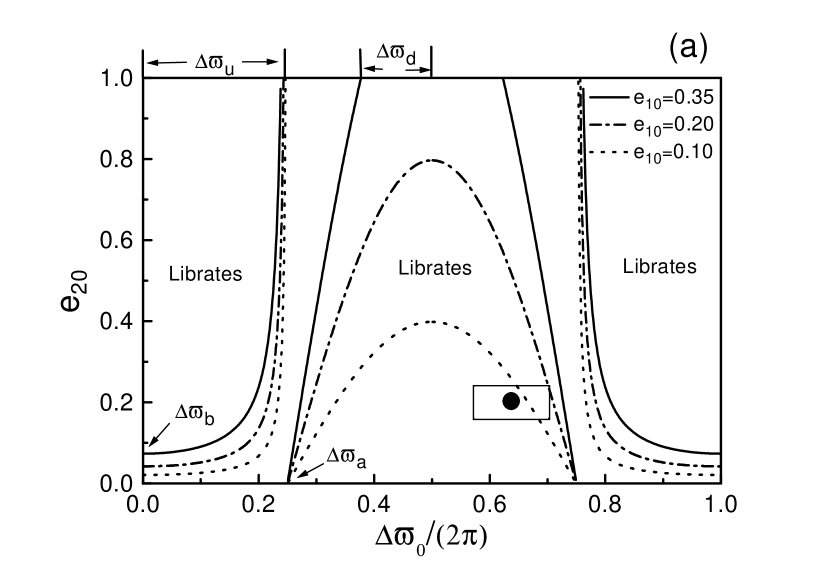
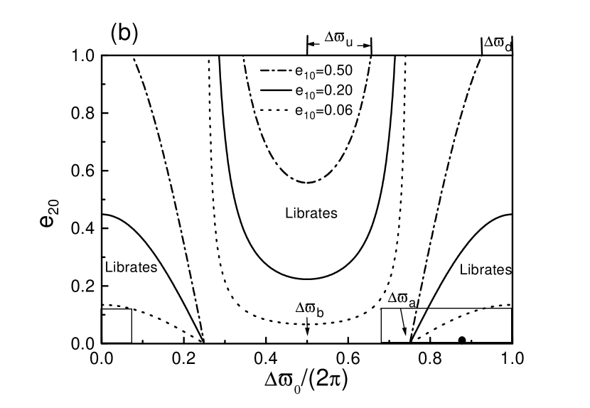
Figure 3: Libration region in $e_{20}-\Delta\varpi_{0}$ plane defined by (19) and (20) with different $e_{10}$ for $\alpha$ and $q$ equal to the planetary system (a) HD12661, and (b) 47 Uma. The black dots show the present configuration of the two planets in both systems, around which the boxes show the uncertainties of the orbital elements in Table 1 and 2. $\Delta\varpi_{a},\Delta\varpi_{b}$ are the lower integration limits in equations (23) and (26), respectively, and $\Delta\varpi_{d},\Delta\varpi_{u}$ are defined in equations (22) and (25), respectively.

We call the libration region defined in (19) the down-libration region, and that defined in (20) the up-libration region. Whether the down-libration or up-libration is the aligned or anti-aligned resonance depends on the sign of $(1-q\alpha^{1/2})$. For $q\alpha^{1/2}<1$, down-libration occurs only when $\pi/2<\Delta\varpi_{0}<3\pi/2$ (thus it is the anti-aligned resonance) and up-libration occurs when $\Delta\varpi_{0}<\pi/2$, $\Delta\varpi_{0}>3\pi/2$ (the aligned resonance). This is the case of HD12661 system. If $q\alpha^{1/2}>1$, the conclusions are reversed, which is the case of 47UMa system. For the critical case $q\alpha^{1/2}=1$, according to (19) and (20), all the orbits are in libration except those with $\Delta\varpi_{0}=\pi/2,3\pi/2$. Fig.2 shows a typical phase space and the evolution of an orbit in the linear secular perturbation system (1). The jumps of $\Delta\varpi$ are due to the cross of origin in the $(e_{i}\cos\varpi_{i},e_{i}\sin\varpi_{i})$ plane. Fig.3 shows the resonance region in the $e_{20}-\Delta\varpi_{0}$ plane defined by (19)(20) with different $e_{10}$. The parameters $\alpha$ and $q$ are taken from the planetary systems HD12661 and 47 UMa(listed in Table 1-2). The boxes around the present configuration dots show the uncertainties of the elements (also listed in Table 1-2).

There are two limit cases for the criteria (19) and (20):

(1) $\alpha\rightarrow 0$. The minimum $e_{20}$ for up-libration and maximum $e_{20}$ for down-libration can be obtained by setting $\cos\Delta\varpi=1$ in (19) and (20). When $\alpha\rightarrow 0$, the minimum $e_{20}$ for up-libration tends to very large and maximum $e_{20}$ for down-libration tends to zero. So when the two planets are far away, the libration regions in $e_{20}-\Delta\varpi_{0}$ plane can be negligible small.

(2) $e_{i0}\rightarrow 0$. This happens when one of the planets is in a near-circular orbit, and it is just the case discussed in Malhotra (2002), namely for two planets initially in nearly circular orbits, an impulse perturbation may impart a finite eccentricity to one planet’s orbit. When $e_{10}\rightarrow 0$, criterion (20) is always fulfilled if $-\pi/2<\Delta\varpi_{0}<\pi/2$ for $q\alpha^{1/2}<1$ or $\pi/2<\Delta\varpi_{0}<3\pi/2$ for $q\alpha^{1/2}>1$. The boundary curves are the limits of those with $e_{10}$ tends to zero in Fig.3a or Fig.3b, with both the minimum $e_{20}$ for up-libration and the maximum $e_{20}$ for down-libration tend to zero. Thus half of the $e_{20}-\Delta\varpi_{0}$ plane is the possible resonance region with up-libration. So the probability of these two planets captured into apsidal resonance tends to $50\%$. This conclusion agrees with that of Malhotra (2002). It’s possible that these two planets are captured in anti-aligned apsidal resonance, which depends on the sign of $1-q\alpha^{1/2}$. Similarly, when $e_{20}\rightarrow 0$, criterion (19) is always fulfilled, thus half of $e_{20}-\Delta\varpi_{0}$ plane are possible resonance region with down-libration, and the probability of the two planets in apsidal resonance (either aligned or anti-aligned resonance) tends to $50\%$.

To compare the above libration regions obtained by the criteria with those calculated from the secular perturbation system, we integrate the orbits of the secular perturbation system for the HD12661 system. Fig.4 shows the diagrams of orbits in $e_{2}-\Delta\varpi$ plane, the initial values of the studied orbits have $e_{10}=0.1$, with $\Delta\varpi_{0}=0$ for Fig.4a and $\Delta\varpi_{0}=\pi$ for Fig.4b. According to the criteria(19) and (20), $e_{20}>0.022$ for the aligned resonance at $\Delta\varpi_{0}=0$, and $e_{20}<0.375$ for the anti-aligned resonance at $\Delta\varpi_{0}=\pi$, which coincide with those given from the secular perturbation system.

Fig.5 shows the contours of the excursions of $e_{1}$,$e_{2}$ for different $e_{20}$ and $\Delta\varpi_{0}$. As we can see, generally the orbits in apsidal resonance have relatively smaller $\Delta e_{1}$, $\Delta e_{2}$, especially the turning points of the contour curves lie in one of libration boundary curves. Thus from the linear secular perturbation theory, the orbits in apsidal resonance, either in aligned resonance or anti-aligned resonance, are more stable than those in non-resonance region.

2.3 Area of the libration region

From the above criteria, we can calculate the probability that the two planets fall in apsidal resonance in the space of initial orbital elements . We define the probability as the area of the libration region in the $e_{20}-\Delta\varpi_{0}$ plane for a given $e_{10}$. For the down-libration case, according to (19), it’s possible that the peak value of the $e_{20}-\Delta\varpi_{0}$ curve can be above unit for larger $e_{10}$ (as the $e_{10}=0.35$ case in Fig.3a, and the $e_{10}=0.50$ case in Fig.3b). We set $\Delta\varpi_{d}$ as the half width of the down-libration region where the boundary curve reaches $e_{20}=1$. Fig.3a and Fig.3b show $\Delta\varpi_{d}$ for the $e_{10}=0.35$ and $e_{10}=0.50$ curves, respectively. Define

$$Q_{d}=\frac{5}{2}\frac{e_{10}q\alpha^{3/2}(1-\frac{1}{8}\alpha^{2})}{|1-q\alpha^{1/2}|},$$ (21)

then,

$$\Delta\varpi_{d}=\left\{\begin{array}[]{ll}\arccos(1/Q_{d}),{}{}&~{}~{}{\rm if}~{}Q_{d}>1\\ 0,{}{}&~{}~{}{\rm if}~{}Q_{d}\leq 1\end{array}\right.$$ (22)

and the area ratio of the down-libration area to the total area of $e_{20}-\Delta\varpi_{0}$ plane is,

$$\begin{array}[]{ll}P_{d}&=\frac{1}{\pi}[\Delta\varpi_{d}+\int_{\Delta\varpi_{a}}^{\Delta\varpi_{a}+\frac{\pi}{2}-\Delta\varpi_{d}}Q_{d}\cos\Delta\varpi~{}d\Delta\varpi]\\ &=\frac{1}{\pi}[\Delta\varpi_{d}+Q_{d}(1-\sin\Delta\varpi_{d})]\end{array}$$ (23)

where the lower integration limit is the beginning point of the down-libration region in $\Delta\varpi_{0}$-axis ($\Delta\varpi_{a}=\frac{\pi}{2}$ for $q\alpha^{1/2}<1$ and $\Delta\varpi_{a}=\frac{3\pi}{2}$ for $q\alpha^{1/2}>1$). Fig.3a and Fig.3b show the $\Delta\varpi_{a}$ for the $e_{10}=0.35$ and $e_{10}=0.50$ curves, respectively. As one can see, the area ratio for the down-libration increases linearly with $e_{10}$ when $e_{10}$ is small, since in the interval one has $\Delta\varpi_{d}=0$ in equation(23). However, for larger $e_{10}$, the increase of area ratio is no longer linear since $\Delta\varpi_{d}\neq 0$.

Similarly, for the up-libration resonance, if we set $\Delta\varpi_{u}$ as the half wide of the up-libration region when the boundary curve meets $e_{20}=1$(see Fig3) and define

$$Q_{u}=\frac{2}{5}\frac{e_{10}|1-q\alpha^{1/2}|}{\alpha(1-\frac{1}{8}\alpha^{2})},$$ (24)

so,

$$\Delta\varpi_{u}=\arccos(Q_{u}),$$ (25)

and the area ratio of the up-libration area to the total area of $e_{20}-\Delta\varpi_{0}$ plane is,

$$\begin{array}[]{ll}P_{u}&=\frac{1}{\pi}[\Delta\varpi_{u}-\int_{\Delta\varpi_{b}}^{\Delta\varpi_{b}+\Delta\varpi_{u}}Q_{u}\frac{1}{\cos\Delta\varpi}~{}d\Delta\varpi]\\ &=\frac{1}{\pi}[\Delta\varpi_{u}-Q_{u}\ln(\frac{1+\sin\Delta\varpi_{u}}{\cos\Delta\varpi_{u}})]\end{array}$$ (26)

where the lower integration limit $\Delta\varpi_{b}$ is the center of the up-libration region ($\Delta\varpi_{b}=0$ for $q\alpha^{1/2}<1$ and $\Delta\varpi_{b}=\pi$ for $q\alpha^{1/2}>1$, see Fig.3).

In the early evolution of planetary systems, both $q$ and $\alpha$ may vary due to planetary formation and migration. We fix $e_{10}=0.35$ for the HD12661 systems, and see the variation of libration area ratio with $\alpha$ or $q$. Fig.6 shows the variation of libration area ratios with $\alpha$ and $q$. In Fig.6a $q\approx 1.46$ is fixed as the observed value. One can see the ratios increase with $\alpha$ before they reach the maximum (unit) at $\alpha_{max}=q^{-2}\approx 0.47$, which is the critical case, and then decrease. In Fig.6b $\alpha\approx 0.32$ is fixed as the observed values. Again the curves reach the maximum at $q=\alpha^{-1/2}\approx 1.76$, the critical case.

3 STABILITY OR ORBITS IN RESONANCE

Since the linear secular perturbation theory is an approximation to the real three-body system, the above criteria obtained from the linear perturbation theory has its limitation. To apply the linear criteria to the predicting of the apsidal secular resonance, we integrate the orbits in a general three-body (co-planar) system, where the longitudes of the ascending nodes and the inclinations of the two planet orbits are assumed to be zero ($\Omega_{1}=\Omega_{2}=0$, $i_{1}=i_{2}=0$) in the paper. We adopt the RKF7(8) (Runge-Kutta-Fehlberg) integrator with adaptive step-sizes to integrate the orbits. Generally the step is alternated between $0.00625$yr and $0.0125$yr, so there are 80-160 steps in a period of planet orbit with a semi-major axis of 1AU, and the final error of the Hamiltonian of the three-body system after $10M$ years’ evolution is less than $10^{-9}$.

We define an index to indicate whether an orbit is in libration region or not. Choose a serial of discrete time during the evolution of orbits (for example, every 12.5 years), give an index $I_{n}$ for each time so that $I_{n}=0$ if at that time $-\pi/2<\Delta\varpi<\pi/2$ and $I_{n}=1$ if $\pi/2<\Delta\varpi<3\pi/2$. Then the average values of $I_{n}$ over very large $n$, denoted by $<I_{n}>$, shows roughly the character of the orbit during the studied period of time according to

$${\rm Index}=<I_{n}>\approx\left\{\begin{array}[]{cc}0&{\rm aligned~{}~{}libration}\\ 0.5&{\rm circulation}\\ 1&{\rm anti-aligned~{}~{}libration}\\ {\rm others}&{\rm mixed}\end{array}\right.$$ (27)

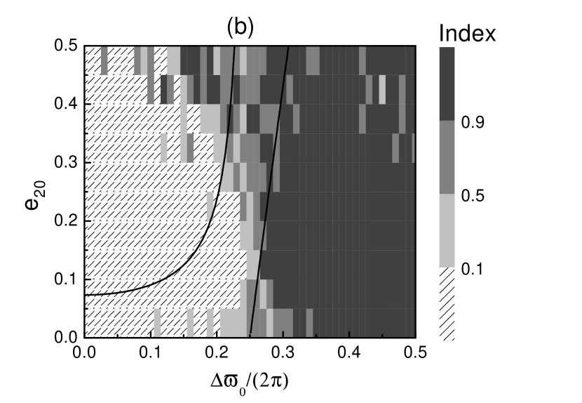
Figure 7: Libration regions in the $e_{20}-\Delta\varpi_{0}$ plane in the general three-body system for the HD12661 system. The solid curves show the boundary defined in (19)(20). The initial eccentricity is (a) $e_{10}=0.10$ and (b)$e_{10}=0.35$.

Fig.7 shows the index for the HD12661 planet system for $10\times 51$ orbits in the interval $[0,0.5]\times[0,\pi]$ of the $e_{20}-\Delta\varpi_{0}$ plane(the same for the following calculations), the initial eccentricity is $e_{10}=0.10$ in Fig.7a and $e_{10}=0.35$ in Fig.7b. As one can see, most of the orbits in the libration region predicted by linear criteria (19) and (20) are in real libration region when $e_{20}$ is small. The discrepancies between the linear system and the three-body one mainly occur on larger $e_{20}$ and the boundary between the libration and circulation region.

Next we want to see whether the orbits, either in apsidal resonance or not, may have different stability in the general co-planar three-body model. The stability of an orbit in a Hamiltonian system is related with the topology (regular or chaotic) of the phase space, so we calculate the largest Lyapunov Characteristic Exponent (LCE) to indicate whether the corresponding orbit is in a regular or chaotic region. The LCE at finite time $\chi(t)$ is calculated for few orbits up to $t=10$Myr (denoted as $\chi_{7}$), and for most orbits up to $t=1$Myr (denoted by $\chi_{6}$). Fig.8 shows the LCEs of four orbits in the four different kinds of region in the phase space. For curve (a), $\chi(t)$ decrease linearly with $t$, thus the orbit corresponding to curve (a) has zero LCE, and is in a regular region. Curve (b) shows a very small but non-zero LCE, so the orbit corresponding to (b) is in a very weak chaotic region. Both curves (a) and (b) have $\chi_{6}\sim 10^{-5}$yr^-1, $\chi_{7}\sim 10^{-6}$yr^-1. Curve (c) tends to a constant value, with $\chi_{6}\approx\chi_{7}\sim 10^{-4}$yr^-1, so the orbit corresponding to (c) should be in a strong chaotic region. The orbit corresponding to curve (d) is unstable with the outer planet escape before $10^{7}$Myr, and $\chi(t)$ for such an orbit is generally great than $10^{-2}$yr^-1 before escape. Thus by calculating $\chi_{6}$ (unit: yr^-1), we can tell at least three different kinds of orbits:

$$\chi_{6}\in\left\{\begin{array}[]{cc}(10^{-5},10^{-4}]&{\rm regular~{}or~{}weak~{}chaos}\\ (10^{-4},10^{-2}]&{\rm strong~{}~{}chaos}\\ (10^{-2},10^{-1}]&{\rm unstable}\end{array}\right.$$ (28)

We calculate $\chi_{6}$ for the HD12661 system with initial eccentricity $e_{10}=0.10$ in one run and $e_{10}=0.35$ in another run, and the other initial parameters are taken as the observed values. Fig.9 show the results. The boundary curves for the corresponding $e_{10}$ are also plotted in the diagram. We find for small $e_{10}$, the orbits, whether in aligned resonance, anti-aligned resonance or non-resonance regions, do not show much difference about the LCEs. So in this case, whether an orbit is in apsidal resonance do not affect much on its stability. However, for larger initial $e_{10}$, orbits in aligned resonance seem to be more stable since they have much lower LCE as compared with those in the anti-aligned resonance or circulation regions with same $e_{20}$. This example shows for larger $e_{10},e_{20}$, planets in aligned resonance regions would be relatively more stable. From Fig.9b, we can also see the present configuration of HD12661b and HD12661c is in the boundary of a chaotic region, if $\Delta\varpi_{0}$ is set to $130.7^{0}$, which is symmetric with the observed value $-130.7^{0}$. This conclusion has been obtained by Kiseleva-Eggleton et al. (2002).

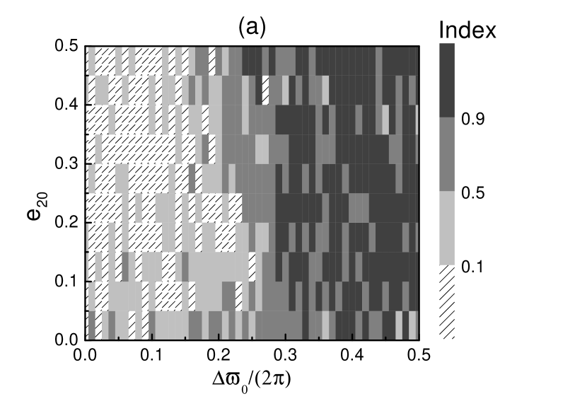
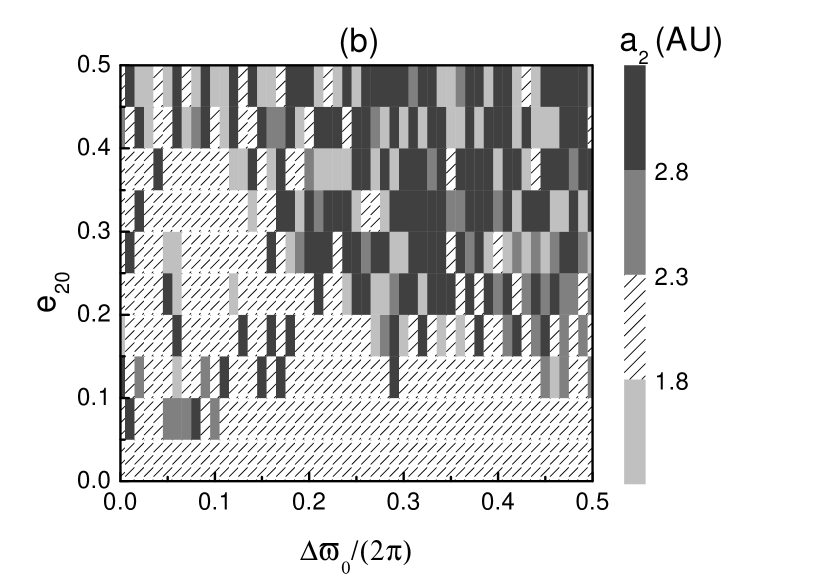
Figure 10: (a) The index of libration region and (b) the relative semi-major axis of two planets HD12661 systems under azimuthal acceleration $f_{2}=-2\times 10^{-6}{\rm AU}^{2}{\rm yr}^{-1}$ . The initial eccentricity is $e_{10}=0.35$ and $M_{10},M_{20}$ are random chosen. The time evolution is $t=50000$yr.

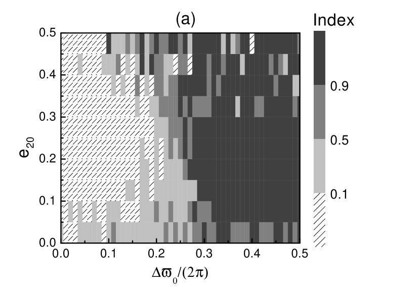
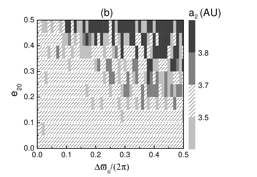
Figure 11: (a) The index of libration region and (b) the relative semi-major axis of two planets HD12661 systems under azimuthal acceleration $f_{2}=-2\times 10^{-6}{\rm AU}^{2}{\rm yr}^{-1}$. The initial eccentricity is $e_{10}=0.35$ and $M_{10},M_{20}$ are random chosen. The evolution time is $t=-50000$yr.

Finally, we study the role of apsidal resonance on the stability of the orbits when the planets are migrating. In the early stage of planet evolution, the protoplanets and the stellar-disk might be coexisting and interacting, thus planet migration might happen due to nebular tides(see, e.g., Ward 1997). We adopt the torqued three-body model as in Laughlin et al. (2002), and for the sake of simplicity, we consider the case that only the outer planet experiences an azimuthal torque due to the planet-disk interaction. We take the azimuthal acceleration as $f_{2}=-2\times 10^{-6}$AU²yr^-1 (which is smaller than that used in Laughlin et al. (2002), because here we concern the qualitative evolutions only), and study both the forward ($t>0$) and backward ($t<0$) evolutions of orbits under this acceleration. We calculate the orbits for the HD12661 system with initial $e_{10}=0.35$, and $M_{10},M_{20}$ are random chosen. All the other initial parameters of orbits are taken from table 1. The evolution time span is $50000$ years. We find in all the studies cases(both forward and backward), the semi-major axis of the inner planet do not have secular changes, just as the results in Laughlin et al. (2002). Fig.10a shows the index for the orbits during the evolution and Fig.10b shows the $a_{2}$ at the final time for the forward case. Some of the orbits which were initially in apsidal resonance region become mixed, though, according to Fig.6a, the libration regions are enlarged due to the increase of $\alpha$ (from 0.32 to approximately 0.41) by planet migration. For orbits in the aligned resonance, they are more stable and with smaller final $a_{2}$, while for orbits in anti-aligned resonance with larger $e_{20}$, or in circulation region, they tend to be more unstable due to close encounters and thus have larger final $a_{2}$, and most of them will escape soon in the following evolutions. Fig.11 shows the backward case. We find the conclusions are more or less similar. Though the libration regions shrink due to the decrease of $\alpha$ by the planet migration (from 0.32 to approximately 0.23) in this case, the configurations of apsidal resonance are generally preserved during the migration. Thus most of planet systems which are observed in apsidal resonance now may be in resonance before the migration begins. Again, the orbits in aligned resonance seem to be more stable in the sense of having modest final $a_{2}$, which may be the results of less close encounters between the two planets.

4 CONCLUSIONS AND DISCUSSIONS

In this paper,we have studied the occurrence as well as the stability of the apsidal resonance. The apsidal resonance occurs when the equations (19)(20) are fulfilled. We find the occurrence of apsidal resonance depends only on the mass ratio $q=m_{1}/m_{2}$, semi-major axis ratio $\alpha=a_{1}/a_{2}$(in secular systems, $a_{1},a_{2}$ are constants), initial eccentricity ratio $e_{10}/e_{20}$ and the relative apsidal longitude $\varpi_{20}-\varpi_{10}$ of the two planets. The criteria are based on the Laplace-Lagrange secular solution of linear perturbation theory. Based on these criteria, the ratio of librating to non-librating orbits in the $e_{20}-\Delta\varpi_{0}$ plane can be obtained analytically, which is given in (23)(26). We also find for two planets on the orbits with large eccentricities, they can be in a stable configuration only when they are in aligned apsidal resonance. When the planets are migrated under the planet-disk interactions, more than half of the studied orbits preserves the configurations of apsidal resonance.

The linear secular perturbation theory is applicable only when the two planets are not in a lower order mean motion resonance. Since in lower order resonances, the variations of $\varpi_{1}$ and $\varpi_{2}$ are not guided by the secular dynamics, but the resonance angles. For example, for the $j:(k-j)$ resonance, if the two resonance angles $\theta_{1}=j\lambda_{1}+(k-j)\lambda-k\varpi_{1}$, $\theta_{2}=j\lambda_{1}+(k-j)\lambda-k\varpi_{2}$ librate around $0$ or $\pi$, then the relative longitude of pericenter $\Delta\varpi=(\theta_{1}-\theta_{2})/k$ must librate around either $0$ or $\pi$. Thus we think in this case, the lower order mean motion resonance and the apsidal resonance are not independent, and the former one guide the dynamics. In the case that only $\theta_{1}$ librates, we believe that the apsidal resonance is very difficult to occur, since in this case $\varpi_{1}$ is guided by $\theta_{1}$, thus it can not have similar variations with $\varpi_{2}$.

Beauge et al. (2002) find that, there may exist some asymmetric stationary solutions in mean motion resonance region, where both the resonant angles and $\Delta\varpi$ are constants with values different from 0 or $\pi$. We think such kind of solutions are due to the mean motion resonance and can only exist in the resonance regions, since such kinds of apsidal resonance solutions with $\Delta\varpi$ librates about constants with values different from 0 or $\pi$ can not be found in the linear secular perturbation system.

For the ten known multiple-planet systems (see Table 8 of Fischer et al. (2003) for a list of the elements), the situation of whether apsidal resonance happens between their planets can be classified roughly into three groups(see Table 3 for the extensions of $\Delta\varpi_{0}$ when apsidal resonance would occur for the observed $q,\alpha,\frac{e_{20}}{e_{10}}$):

(1) planets both in apsidal resonance and mean motion resonance. 55 Cancri b and c (Fig.12a), GJ876 b and c , HD82943 b and c are in apsidal resonance since they are in mean resonances 3:1, 2:1 and 2:1 respectively. In fact, HD82943 b and c can in apsidal resonances without in the mean motion resonance, while GJ876 b and c are near the boundary of libration according to the linear secular dynamics(Fig.13a).

(2) planets in apsidal resonances far away from lower order mean motion resonances. HD12661 b and c, 47 UMa b and c, Ups And c and d(Fig.12b) are in this type. They are in apsidal resonance without the existence of any strong mean resonances. Moreover, HD12661 b and c seems to be in anti-aligned apsidal resonance, which is in the boundary of a chaotic region.

(3) planets not in apsidal resonance either due to the negligible small libration region in the $e_{20}-\Delta\varpi_{0}$ plane or without suitable $\Delta\varpi_{0}$. The two planets in HD38529, HD168443, HD74156 are not in apsidal resonance, since the libration regions in the $e_{20}-\Delta\varpi_{0}$ are negligible small for the observed $q$,$\alpha$ and $e_{2}/e_{1}$(Table 3). HD37124 b and c have large aligned libration area for the present parameters, and their eccentricities are not small, but they are not in resonance due to the present values of $\Delta\varpi_{0}$ if $\Omega_{b}=\Omega_{c}=0$ are assumed (Fig.13b).

However, due to the unknown of the inclinations and the longitude of ascending nodes in the orbital fit from the observation data, it is still too early to make conclusions for some planet systems whether the planets are in apsidal resonances. For example, for the HD12661 b and c, they are believed to be in the anti-aligned libration now. This is achieved by assuming $\Omega_{1}=\Omega_{2}=0$, and they are in the boundary of a chaotic region. Alternative choices of $\Omega_{i}$ (i=1,2) may change the conclusion. Especially if we chose $\Omega_{1}-\Omega_{2}\sim 180^{0}$, the two planets will in the aligned apsidal resonance , which is stable according to Fig.9b. Similarly, HD37124 b and c could in apsidal resonance if suitable parameters $\Omega$ are observed.

Similar secular resonance may also happen due to nearly the same averaging precessing rate of the ascending nodes between the two planets in mutually inclined orbits. Since the inclination perturbations are isolated from the eccentricity ones in the linear secular perturbation theory, we will address this problem in a separate paper (Zhou and Sun, in preparation).

Figure 1: The approximation of $c_{0}$ in equation (3)

Figure 2: The critical case of HD12661 with the observed $a_{1}$ and $q$ but with $a_{2}=a_{1}q^{2}\approx 1.76AU$. (a) The phase plane $e_{2}-\Delta\varpi$, the orbits in the diagram have the same constant $D$ as that of $e_{10}=0.35,e_{20}=0.20$. (b)Variation of $e_{1},e_{2},\Delta\varpi$ with time for an orbit with $\Delta\varpi_{0}=\pi/2.$

Figure 4: Orbital diagrams of planet system HD12661 with initial values (a) $e_{10}=0.1$,$\Delta\varpi_{0}=0$; (b)$e_{10}=0.1$,$\Delta\varpi_{0}=\pi$

Figure 5: Contours of $\Delta e_{1},\Delta e_{2}$ defined by (14) in the initial $e_{20}-\Delta\varpi_{0}$ plane with $e_{10}=0.35$. The dotted lines are the boundary of the libration region defined in (19)(20).

Figure 6: Variations of the libration area ratios with $\alpha$ and $q$ for the planet system HD12661. (a) the observed $q\approx 1.46$ is fixed, and (b) the observed $\alpha\approx 0.32$ fixed. In both diagrams $e_{10}=0.35$ is fixed. The black dot in each plot shows the location of observed configuration.

Figure 8: The LCE $\chi(t)$ for (a) the 47Umas system with the observed orbital parameters listed in Table 2; (b) the HD12661 system with the observed orbital parameters listed in table 1; (c) same parameters as in (b) except $e_{20}=0.20$, $\varpi_{10}=0$, $\varpi_{20}=0.6\pi$; (d) same parameters as in (b) except $e_{20}=0.35$, $\varpi_{10}=0$, $\varpi_{20}=0.7\pi$, the outer planet is escape at time $t\approx 2.1\times 10^{5}$yr.

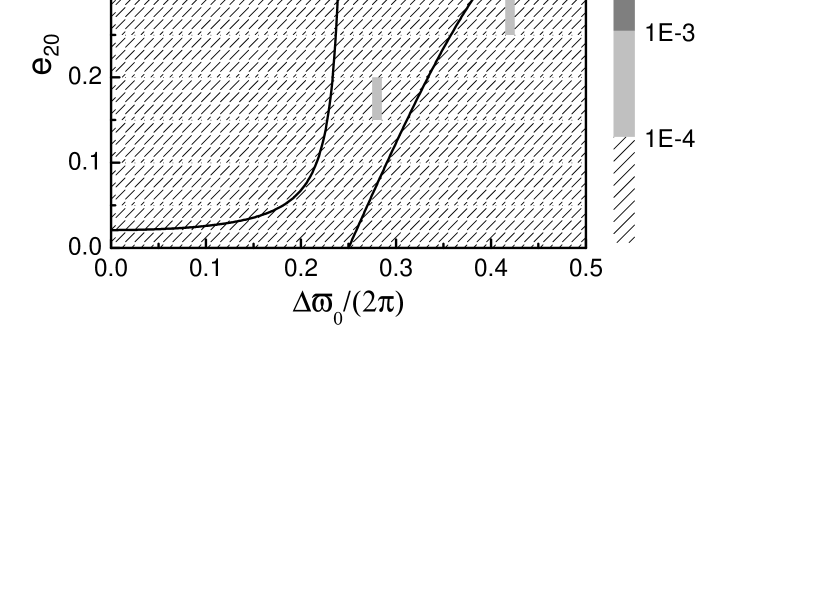
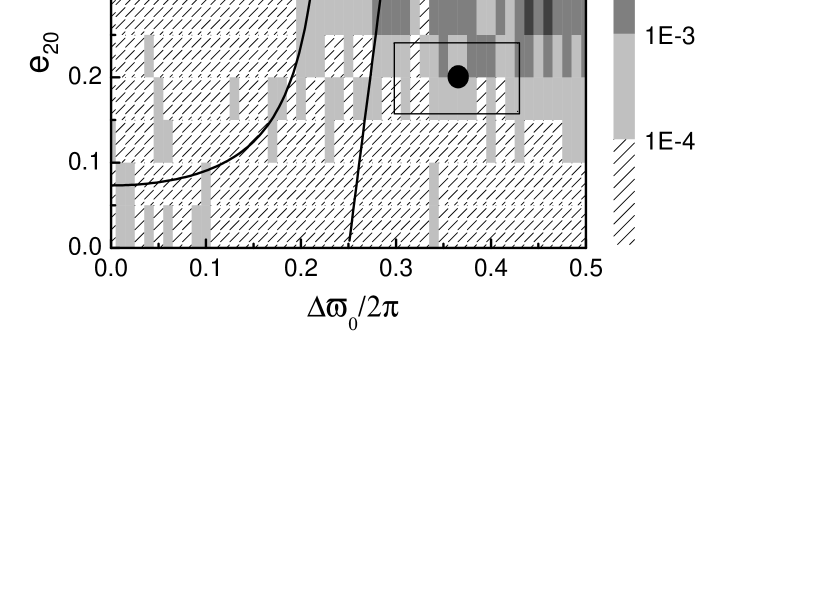
Figure 9: The LCE $\chi_{6}$ for HD12661 system. The initial eccentricity is(a) $e_{10}=0.10$, (b)$e_{10}=0.35$. The solid curves show the boundary defined in (19)(20). The black dot in (b) shows the location of observed configuration with $\Delta\varpi_{0}=130.7^{o}$, around which the box show the uncertainties of the orbital elements.

Figure 12: Libration region in the initial $e_{20}-\Delta\varpi_{0}$ plane defined by (19) and (20) for the two triple-planet systems (a)55 Cancri ($\varpi_{b}=99^{0}$,$\varpi_{c}=61^{0}$,$\varpi_{d}=201^{0}$); (b) Upsilon Andromedae ($\varpi_{b}=73^{0}$,$\varpi_{c}=250^{0}$,$\varpi_{d}=260^{0}$). Invisible boundary curves are out of the range of $e_{20}$. The black dots show the present configuration of the two planets. Other orbital elements are taken from Fischer et al. (2003).

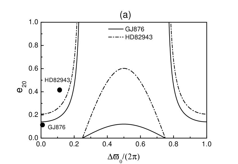
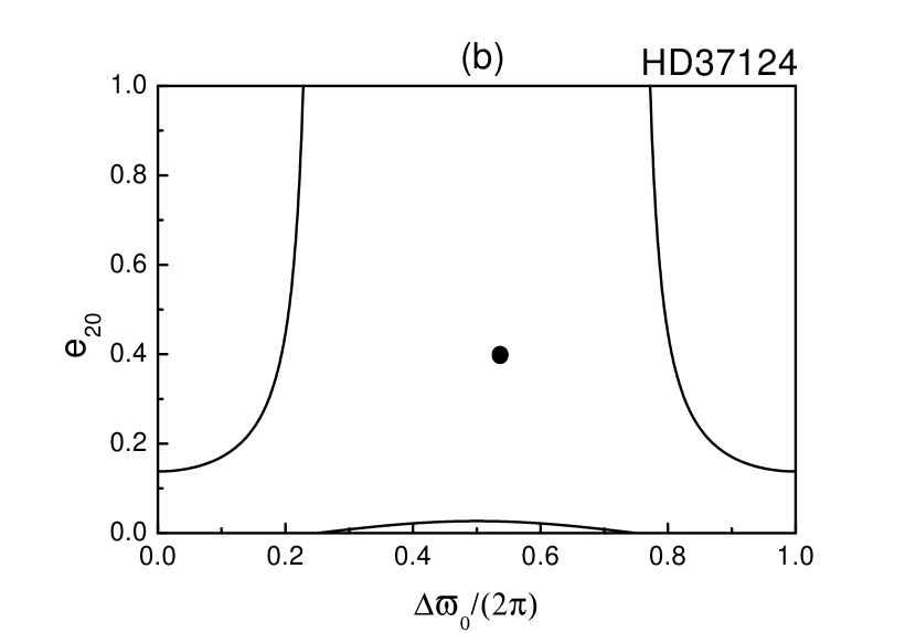
Figure 13: Libration region in the initial $e_{20}-\Delta\varpi_{0}$ plane defined by (19) and (20) for the planetary system (a) GJ876 ($\varpi_{b}=330^{0}$,$\varpi_{c}=333^{0}$),HD82943 ($\varpi_{b}=96^{0}$,$\varpi_{c}=138^{0}$); (b) HD37124 ($\varpi_{b}=60^{0}$,$\varpi_{c}=259^{0}$). The black dots show the present configuration of the two planets. Other orbital elements are taken from Fischer et al. (2003).

Table 1: Orbital Parameters  for HD12661(1.07M_⨀) system

Parameter	HD12661 b	HD12661 c
planet mass M$\sin i$ (Mjup)	2.30	1.57
period P(days)	263.6(1.2)	1444.5(12.5)
Tp (JD) (days)	2,449,941.9(6.2)	2,449,733.6(49.0)
semi-major axis a (AU)	0.82	2.56
eccentricity e	0.35(0.03)	0.20(0.04)
argument of pericenter $\omega$ (deg)	293.1(5.0)	162.4(18.5)

Table 2: Orbital Parameters  for 47UMa(1.03M_⨀) system

Parameter	47UMa b	47 UMa c
planet mass M$\sin i$ (Mjup)	2.54	0.76
Period P(days)	1089.0(2.9)	2594(90)
Tp (JD) (days)	2,450,356.0(33.6)	2,451,363.5(495.3)
semi-major axis a (AU)	2.09	3.73
eccentricity e	0.061(0.014)	0.005(0.115)
argument of pericenter $\omega$ (deg)	171.8(15.2)	127.0(55.8)

Table 3: Extensions of $\Delta\varpi_{0}$ in apsidal resonance for the observed systems

Planet Pair	$q=\frac{m_{1}}{m_{2}}$	$\alpha=\frac{a_{1}}{a_{2}}$	$\frac{e_{10}}{e_{20}}$	aligned $\Delta\varpi_{0}$	anti-aligned $\Delta\varpi_{0}$
Ups And b-c	0.358	0.0720	0.037	(-79.3o,79.3o)	-
Ups And b-d	0.181	0.0228	0.040	(-47.0o,47.0o)	-
Ups And c-d	0.507	0.317	1.08	(-9.0o,9.0o)	-
55 Cnc b-c	4.15	0.477	0.073	-	(96.8o,263.2o)
55 Cnc b-d	0.225	0.021	0.107	-	-
55 Cnc c-d	0.054	0.044	1.46	-	-
GJ876 c-b	0.296	0.628	2.70	-	(144.0o,216.0o)
47 UMa  b-c	3.34	0.560	12.2	(-87.9o,87.9o)	-
HD37124 b-c	0.860	0.184	0.250	(-69.8o,69.8o)	-
HD12661 b-c	1.46	0.320	1.75	(-67.8o,67.8o)	(98.6o,261.4o)
HD82943 c-b	0.540	0.628	1.32	(-59.7o,59.7o)	(132.8o,227.2o)
HD168443 b-c	0.450	0.103	2.65	-	-
HD38529 b-c	0.061	0.035	0.806	-	-
HD74156  b-c	0.208	0.080	1.625	-	-

References

- Beague,Ferraz-Mello,& Michtchenko (2003) Beauge,C.,Ferraz-Mello,S.,& Michtchenko,T.A. 2003,ApJ,accepted
- California and Carnegie Planet Search (2003) California and Carnegie Planet Search 2003,http://exoplanets.org/planet_table.shtml
- Chiang, Tabachnik,& Tremaine (2001) Chiang, E.I., Tabachnik, S.,Tremaine,S. 2001, AJ,122,1607
- Fischer et al. (2002) Fischer,D.A.,Marcy,G.W.,Butler,R.P.,Laughlin,G.,Vogt,S.S. 2002,ApJ,564,1028
-
Fischer et al. (2003)
Fischer,D.A.,Marcy,G.W.,Butler,R.P.,Vogt,S.S.,Henry,G.W.,Pourbaix,D.,Walp,B.,
Misch,A.A.&Wright J.T. 2003,ApJ,586,1394 - Goździewski & Maciejewski (2001) Goździewski,K.,&Maciejewski,A.J. 2001,ApJ,563,L81
- Goździewski & Maciejewski (2003) Goździewski,K.,&Maciejewski,A.J. 2003,ApJ,586,L153
- Ji et al. (2003) Ji J. H., Kinoshita H., Liu L. , Li G.Y. 2003, ApJ 585, L139
- Kiseleva-Eggleton et al. (2002) Kiseleva-Eggleton,L.,Bois,R.,Rambaux,N.,&Dvorak,R. 2002,ApJ,578,L145
- Laughlin, Chambers, & Fischer (2002) Laughlin,G.,Chambers,J.&Fischer,D. 2002,ApJ 579, 455
- Lee & Peale (2002) Lee,M.H.,&Peale,S.J. 2002,ApJ,567,596
- Lee & Peale (2003) Lee,M.H.,&Peale,S.J. 2003,ApJ,592,1201
- Malhotra (2002) Malhotra,R. 2002,ApJ,575,L33
- Marcy et al. (2001) Marcy,G.W.,Butler,R.P.,Fischer,D.A.,Vogt,S.S.,Lissaur,J.J.,&Rivera,E. 2001,ApJ,556,296
- Murray & Dermott (1999) Murray,C.D.,& Dermott,S. F. 1999, Solar System Dynamics (Cambridge: Cambridge university Press) 274
- Ward (1997) Ward,W.R. 1997,Icarus,126,261