Cool White Dwarfs Revisited – New Spectroscopy and Photometry

Abstract

In this paper we present new and improved data on 38 cool white dwarfs identified by Oppenheimer et al. (2001) (OHDHS) as candidate dark halo objects. Using the high-resolution spectra obtained with LRIS on Keck I, we measure precise radial velocities for 13 white dwarfs that show an ${\rm H}\alpha\,$absorption line. We show that the knowledge of radial velocities on average decreases the $UV$-plane velocities by only 6%. In two cases the radial velocities put original halo candidates below the OHDHS velocity cut. The radial velocity sample has a velocity dispersion in the direction perpendicular to the Galactic plane of $\sigma_{W}=59\,{\rm km}\,{\rm s}^{-1}$ – in between the values typically associated with the thick disk and the stellar halo populations. We also see indications for the presence of two populations by analyzing the velocities in the $UV$ plane. In addition, we present CCD photometry for half of the sample, and with it recalibrate the photographic photometry of the remaining white dwarfs. Using the new photometry in standard bands, and by applying the appropriate color-magnitude relations for hydrogen and helium atmospheres, we obtain new distance estimates. By recalibrating the distances of the white dwarfs that were not originally selected as halo candidates, we obtain 13 new candidates (and lose 2 original ones). On average, new distances produce velocities in the $UV$ plane that are larger by 10%, with already fast objects gaining more. Using the new data, while applying the same $UV$-velocity cut ($94\,{\rm km}\,{\rm s}^{-1}$) and methods of analysis as in OHDHS, we find a density of cool white dwarfs of $1.7\times 10^{-4}\,{\rm pc}^{-3}$, confirming the value of OHDHS. In addition, we derive the density as a function of the $UV$-velocity cutoff. The density (corrected for losses due to higher $UV$-velocity cuts) starts to flatten out at $150\,{\rm km}\,{\rm s}^{-1}$ ($0.4\times 10^{-4}\,{\rm pc}^{-3}$), and is minimized (thus minimizing a possible non-halo contamination) at $190\,{\rm km}\,{\rm s}^{-1}$ ($0.3\times 10^{-4}\,{\rm pc}^{-3}$). These densities are in a rough agreement with the estimates for the stellar halo white dwarfs, corresponding to a factor of 1.9 and 1.4 higher values.

Accepted to ApJ

1 Introduction

Dynamical studies indicate that the large quantities of gravitating matter exist in the haloes of galaxies, including our own. The amount of this matter far surpasses the matter with detectable electromagnetic radiation. Revealing the nature of this so called “dark matter” is one of the crucial goals in present-day astronomy and cosmology.

One of the first proposed methods to indirectly detect dark matter was to look for lensing of background stars by the dark objects in the halo (Paczyński, 1986). This technique, microlensing, is sensitive to macroscopic objects, known as MACHOs, ranging in mass from planetary to stellar. At the time when the first microlensing experiments began, there was still no consensus as to whether the dark matter haloes should be baryonic or non-baryonic. With the exception of primordial black holes, microlensing would exclusively detect the baryonic matter. Now, after years of observing, microlensing has ruled out a dark halo made entirely of MACHOs, but has nonetheless found more lensing events than expected from the known stellar populations, either in the Galactic disk and halo, or in the LMC (or SMC), where the lensed stars reside. The latest estimate from the MACHO group favors a halo in which dark objects comprise 20%, each with a typical mass of $0.6M_{\odot}$ (Alcock et al., 2000). Another microlensing experiment, EROS, puts upper limits for compact halo objects with stellar masses of 30%, from monitoring the LMC (Lasserre et al., 2000), and 25% from SMC (Afonso et al., 2003). Some researchers (e.g., Sahu 1994) believe that lenses responsible for these events reside in the LMC (or SMC) itself, however these scenarios have their own problems.

Since the search for dark matter in the form of MACHOs began, our paradigms about what the cosmological dark matter should be have changed. With the discovery of cosmological acceleration due to “dark energy” (Garnavich et al., 1998; Riess et al., 1998), the discrepancy between the critical mass density required by the inflationary model, and the low observed densities of gravitating matter was reconciled. Cosmological models preferred the genuine dark matter to be in the form of non-baryonic cold dark matter, concentrated in galactic haloes. On the other hand, the large fraction, or all of the baryonic matter that was previously unaccounted for, is now believed to reside in the systems such as those responsible for the population of Ly $\alpha$ absorbers.

This alone should be enough to shift the focus on the detection of non-baryonic halo dark matter (in the form of particles), were it not for the MACHO results suggesting unknown, dark objects. For the problem to be more severe, there are a number of theoretical and observational arguments suggesting that the baryonic matter should at best constitute only a negligible fraction of the dark halo, much lower than required to explain the fraction of it believed to be in MACHOs (Freese, Fields, & Graff, 2000). Of the various candidate counterparts to MACHOs, ancient, cool white dwarfs are nevertheless the best ones, especially since their expected masses are comparable. The main question then, is, whether we can detect these halo white dwarfs, and if so, what fraction of the dark halo mass do they constitute. Ideally, these white dwarfs should account for all MACHOs; otherwise yet another form of baryonic dark matter is required.

Surveying 10% of the sky, and using a proper-motion selected sample of objects with high reduced proper motions, Oppenheimer et al. (2001) (hereafter OHDHS) have identified and spectroscopically confirmed 98 white dwarfs, of which 38 have halo-like kinematics based on the derived velocity components in the plane of the Galaxy ($UV$ plane). The derived mass density of these cool white dwarfs indicated that they make up at least $\sim 2\%$ of the local dark-matter halo density, an order of magnitude higher than expected from the population of the stellar halo (as opposed to dark halo) white dwarfs (WDs). Stellar halo WDs should differ from the dark halo ones in their origin, since the dark halo white dwarfs were presumably produced in an early burst of star formation, and were cooling ever since. The OHDHS paper and its results stirred the astronomical community, generating numerous objections – regarding the selection of objects, kinematical cuts, contamination from non-halo populations, and so on. A thorough review on the subject of cool white dwarfs, and of various interpretations of OHDHS work is given by Hansen & Liebert (2003).

In this paper, we re-analyze the OHDHS sample of cool white dwarfs using newly acquired high resolution spectra and CCD imaging. The new data allow measurement of radial velocities and determination of photometric distances in a more direct and precise manner, thus addressing some issues raised with respect to original OHDHS data. (The OHDHS used classification-grade, low resolution spectra, and photometry derived from photographic plates).

In §2 we present spectroscopic observations, and the derivation of radial velocities for white dwarfs exhibiting spectral features. Photometry from the CCD imaging is presented in §3, together with a calibration of photographic magnitudes used by OHDHS. In §4 we assemble all data to produce a new dataset required for kinematical analysis. Finally, in §5 we discuss the properties of the revised kinematical dataset, and use it to address some of the issues raised against the original OHDHS sample and its interpretation. In particular, we recalculate the densities of WDs using the OHDHS velocity cut, but also as a function of the cutoff velocity. In a forthcoming work the new dataset will be analyzed with additional techniques, including the kinematical modeling of stellar populations.

2 Spectroscopy

2.1 Observations and data reduction

The spectra of OHDHS cool white dwarfs were taken with the LRIS (Oke et al., 1995) spectrograph on Keck I, on three nights: 2002 Sept 13, 14 and 2002 Dec 4 (UT). The primary goal was to obtain high resolution spectra in the region around the ${\rm H}\alpha\,$line ($\lambda 6563$). Thus, the spectroscopic setup in the red arm of LRIS consisted of 1200/7500 grating, giving dispersion of 0.63 Å  ${\rm pix}^{-1}$, and a spectral coverage of 5850–7140 Å. The only exceptions to this setup were in the cases of WDs with peculiar spectra (that happen to show no hydrogen lines): WD2356-209 and LHS 1402. The first was imaged in both the hi-res and the low-res modes, while the second only in the low-res: 300/5000 grating, 2.46 Å  ${\rm pix}^{-1}$ dispersion, and 5010–10030 Å  range. The slit width of $1^{\prime\prime}$ gave the effective resolution in hi-res mode of 2.9 Å. On 2002 Dec 4 one additional WD was observed (WD2346-478), this time with the 831/8200 grating (0.92 Å  ${\rm pix}^{-1}$ dispersion, 5630–7500 Å  range).

The cumulative exposure times varied from 6 to 45 minutes. Calibration lamp spectra were obtained at each pointing, and the internal-lamp flat-field images were taken once a night. Standard extraction and calibration IRAF tasks were employed to produce the final spectra.

2.2 Measuring radial velocities

Measuring the radial velocities was the main goal of the hi-res spectroscopy observing program. Targets were selected by inspecting the low-res spectra obtained by OHDHS. They found an ${\rm H}\alpha\,$line in 14 out of 38 cool WDs (denoted with an asterisk in OHDHS Table 1). Of these 14, all but three can be observed from Keck’s latitude, and we have obtained spectra of all 11. In addition, we took spectra of another 12 WDs, thought to be featureless. Among these we find an additional two with an ${\rm H}\alpha\,$line. Thus our radial velocity sample comprises of 13 cool WDs.

The wavelength region covered by the hi-res spectra would allow detection of lines other than that of hydrogen (such as He and C). However, careful inspection of the spectra (with S/N ranging from $\sim 30$ to $\sim 110$) does not reveal any such lines.

Each individual spectrum was wavelength calibrated against a lamp spectrum. The typical RMS of the calibration was 0.02 Å. The wavelengths of lines were first measured on individual spectra (of a same object) in order to evaluate the stability of the zero point of wavelength calibration, and to establish the accuracy with which the central wavelength of ${\rm H}\alpha\,$could be determined. All measurements were done using the “splot” routine in IRAF. White dwarf spectra were normalized by the continuum, and a Lorentzian function was used to fit the lines.

The stability of the zero point of the calibration was determined by measuring a bright sky emission line of [OI] at 6300.304 Å. The measured mean wavelength was $6300.30\pm 0.01$ Å, indicating no systematic shifts in the calibration, while the scatter around the mean of 0.07 Å  (equivalent to $3\,{\rm km}\,{\rm s}^{-1}$) gives the level of radial velocity error due to the wavelength calibration.

The spectra of white dwarfs have different levels of signal to noise ratio, leading to variations in the quality of the ${\rm H}\alpha\,$profile. In well exposed spectra, the non-LTE core of ${\rm H}\alpha\,$line will be well defined, so measuring the central wavelength of the core would be superior to fitting a profile to the entire line. However, in lower S/N spectra the core may be degraded by noise. In order to test which method is more appropriate for our sample, we compared line fitting to the entire profile (6400–6800 Å) (which was fitting the wing portions of the profile well, but often failed to fit the core), to the fitting of the non-LTE core alone (width $\sim 5$ Å). For each method, we first find the difference of the individual measurements with respect to the mean value (for the given object), and then calculate the overall scatter. For wide-profile fitting the scatter is 0.45 Å, while for core fitting it is 0.32 Å. In other words, core fitting seems to have better repeatability, and should thus be more precise. We should also note that we do not observe cases of split cores or of emission in the cores.

Since the scatter, i.e., the error of the individual measurements, is much larger than the stability of the zero point of wavelength calibration, we conclude that it is safe to combine the spectra belonging to the same object (between three and six), thus obtaining a higher signal and eliminating deviant points by performing sigma clipping. Since the spectra of a given object were taken over a short period of time, the heliocentric velocity correction need not be applied at this stage. We then proceed by finding central wavelengths of ${\rm H}\alpha\,$lines in the combined spectra, again by fitting a Lorentzian to the core. This gives our final measured wavelength. In order to evaluate the measurement error, we evaluate, as a function of a measured flux, the RMS scatter of the central wavelengths of individual spectra belonging to a given object. Not surprisingly, the scatter is larger for objects whose individual spectra had low intensities. We find a linear relation between the logarithm of flux and the RMS scatter of individual wavelength measurements. However, at a certain flux level the RMS reaches a minimum value of 0.13 Å, despite the increase of signal. In the fluxes of the combined spectra this plateau is actually reached for most spectra in our sample. Thus for most spectra, the total error from noise and wavelength calibration uncertainties is equivalent to $\approx 7\,{\rm km}\,{\rm s}^{-1}$, well within the limits acceptable for this study. Finally, to get the measured radial velocity, we apply the heliocentric correction. The observed radial velocities of 13 WDs and their errors are listed in Table 1. Also listed are 10 WDs observed with LRIS, but lacking spectral features.

3 Photometry

3.1 Observations and data reduction

Photometry was performed on CCD images taken at the 1 m Nickel Telescope at the Lick Observatory, on 2002 Nov 27, Dec 3 and 4 (UT). “Dewar#2” CCD with a high quantum efficiency extending to blue wavelengths was used. The first two nights were fully photometric and many standards over a large range of airmasses and colors were observed. This allowed construction of photometric transformations with linear and quadratic color-terms. The photometric accuracy from calibration is 0.01–0.02 mag in all bands.

Of the 38 cool WDs, 19 reach an altitude high enough to be observed with this telescope. Of them, 18 were imaged in $V$ and $I$ (Cousins) bands. In addition, 9 of those were also observed in $B$ band, and further 3 in $R$ band. Of the 18 WDs with $VI$ photometry, 9 also belong to the radial velocity sample.

Object photometry was performed with an aperture equal to 1 FWHM of the PSF (typically $2\farcs 4$), and then aperture-corrected using a bright isolated star in the field. All $I$-band images were corrected for fringing. For each measurement a photon error from the object was combined with a photon error of the aperture-correction star. The individual measurements were transformed into standard magnitudes and combined (weighted by photometric errors) into a single magnitude per star per band. Median photometry errors of the WD sample are $\langle\sigma_{B}\rangle=0.053$, $\langle\sigma_{V}\rangle=0.035$, $\langle\sigma_{R}\rangle=0.030$, $\langle\sigma_{I}\rangle=0.035$. The median error of $V-I$ color, which we will use to deduce distances, is 0.052 mag. The photometry is summarized in Table 2.

Since most of the cool WDs were not known before, it is not surprising that the literature search for photometric data produced prior measurements for only two WDs: LHS 542 and LHS 147. The comparison of their photometry to ours is given in Table 3. It is in excellent agreement. Photometric magnitudes in other bands do exist for several WDs in SDSS DR1, and for nine WDs in the 2MASS All-Sky Point Source Catalog. The 2MASS measurements will be discussed in §4.3.1.

3.2 Photometric calibration of OHDHS magnitudes

Since we obtained CCD photometry for only one half of the OHDHS sample, it would be useful to derive photometry of other objects in standard bands. Thus, we would like to construct empirical transformations between the photographic plate magnitudes used by OHDHS: $B_{\rm J}$, $R_{\rm 59F}$, and $I_{\rm N}$, and the standard photometric bands. Empirical transformations between photographic and standard magnitudes do exist in the literature, while the synthetic transformations can be constructed using the model spectra and the transmission curves, yet the first method has not been specifically applied to stars such as cool WDs, while the second suffers from often ill-defined properties of the actual response of a given plate/filter combination.

Here we derive relations between photographic and standard magnitudes as measured by CCD photometry.

For $B_{\rm J}$:

$$B_{\rm J}=B-0.85\,(B-V)+0.26.$$ (1)

This relation has $\sigma=0.10$. Since we know that $\sigma_{B}=0.05$, this indicates that $\sigma_{B_{\rm J}}=0.08$, which is quite remarkable for the photographic photometry. Note that a high color-term indicates that (at least for WDs), $B_{\rm J}$ is actually closer to standard $V$ than to standard $B$.

For $R_{\rm 59F}$:

$$R_{\rm 59F}=V-0.66\,(V-I)+0.13.$$ (2)

Since we have our $R$ for only 3 objects, we give this transformation relative to $V$. Excluded from the fit is LHS 1402 – a peculiar WD. Derived accuracy of the relation is 0.10 mag, while $\sigma_{R_{\rm 59F}}=0.09$.

For $I_{\rm N}$:

$$I_{\rm N}=I-0.09\,(V-I)+0.12.$$ (3)

This relation has $\sigma\approx\sigma_{I_{\rm N}}=0.16$. Excluding objects for which OHDHS derive $I_{\rm N}$ spectrophotometrically does not change the above relation.

Another source of photographic magnitudes is the recently completed USNO-B catalog (a similar catalog, GSC-2.2, does not go deep enough in most cases). We have matched all the objects to counterparts in USNO-B catalog (Monet et al., 2003), and repeated the above analysis against $B_{2}$, $R_{2}$ and $I_{\rm SERC}$ – second generation sky survey magnitudes from USNO-B. However, we find that USNO-B magnitudes are significantly inferior to those used by OHDHS, despite the fact that they come from similar or same plate material. Namely, we find $\sigma_{B_{2}}=0.41$, $\sigma_{R_{2}}=0.58$, and $\sigma_{I_{\rm SERC}}=0.26$.

Overall, we conclude that the OHDHS (that is, SuperCOSMOS Sky Survey from which it is taken, Hambly, Irwin, & MacGillivray 2001; Hambly, Davenhall, Irwin, & MacGillivray 2001) photographic plate photometry is of excellent quality, which lends credence to transforming them into standard magnitudes in order to derive photometric distances.

Since we will be obtaining distances from $V$ magnitude and $V-I$ color, we want to directly transform OHDHS magnitudes and colors to these. We have seen that $B_{\rm J}$ is quite close to $V$, so we use that magnitude to obtain the transformations

$$V=B_{\rm J}-0.23\,(B_{\rm J}-I_{\rm N})-0.17,\qquad\sigma=0.12,$$ (4)

$$V-I=0.62\,(B_{\rm J}-I_{\rm N})-0.04,\qquad\sigma=0.08.$$ (5)

These calibrations were derived omitting both peculiar-spectra WDs (LHS 1402 and WD2356-209).

4 The new dataset

4.1 Radial velocities

4.1.1 Gravitational redshifts

The observed radial velocities (Table 1) were extracted as explained in §2. However, they do not represent the true radial velocities, since WDs exhibit substantial gravitational redshift. The exact redshift depends on the mass and the radius of a WD, which we do not know for individual WDs in our sample. However, it is known that the range of these values is relatively small, so for our purposes it is sufficient to adopt a common value for the redshift. From Reid (1996) we find that the field WDs have an average redshift of $28.6\,{\rm km}\,{\rm s}^{-1}$, with a spread of $6.5\,{\rm km}\,{\rm s}^{-1}$. We subtract this value from the observed radial velocities, and add the scatter to the radial velocity measurement error. The final values are listed in Table 4.

4.1.2 Common proper motion binaries

In a case where a WD has a common proper motion companion that is a main sequence star, one can obtain a measurement of a true radial velocity of a white dwarf (whether it contains spectral lines or not) by simply measuring the radial velocity of the main sequence component. Such a measurement circumvents the gravitational redshift correction. To this end, we have carried out a search for companions in the USNO-B catalog, which lists proper motions based on multiple plates. Within the $2^{\prime}$ search radius we find no candidate companions with proper motions compatible to those of the white dwarfs.

4.1.3 Selection effects

The original OHDHS selection of cool WDs was based on the $U$ and $V$ components of the velocity. In the absence of radial velocities, they were calculated by assuming $W=0$. Since our goal is to characterize this population by obtaining the third component of the velocity from the radial velocities, we should try to evaluate whether the subsample for which radial velocities are measured is representative of the population as a whole. Here we will restrict ourselves to a question of whether the subsample is representative kinematically – in terms of its $U$ and $V$ velocities, based on which the cool WD sample was selected in the first place.

OHDHS selected their sample by requiring the WDs to have a velocity above some threshold in the $UV$-plane. This threshold was chosen as $2\sigma$ $UV$ velocity of the thick disk population

$$UV\equiv\sqrt{U^{2}+(V+35\,{\rm km}\,{\rm s}^{-1})^{2}}>94\,{\rm km}\,{\rm s}^{-1}.$$ (6)

One way of characterizing if the subsample of 13 WDs with radial velocities is representative, is to compare its average $UV$ velocity with the typical $UV$ velocities of randomly selected subsamples of 13 WDs out of the total 38.

In order to obtain the distribution of $UV$ velocities of random subsamples, we run a Monte Carlo simulation that draws 13 out of 38 WDs numerous times, and for each drawing calculates its average $UV$ velocity. The average is taken in two ways: as a straight average, and as a weighted average, where weights are the corresponding maximal volumes ($\langle UV\rangle=(\sum(UV/{\mathbf{V}}_{\rm max}))/(\sum(1/{\mathbf{V}}_{\rm max}))$) in which a WD could have been detected in the OHDHS survey. As explained in OHDHS, for each individual object, ${\mathbf{V}}_{\rm max}$ is set either by the magnitude limit of the survey, or by the lower proper motion cutoff, whichever is smaller. In Figure 1, the solid line represents the distribution of unweighted averages. The unweighted average of the radial velocity sample is $195\,{\rm km}\,{\rm s}^{-1}$, and is indicated by the arrow. We see that it is on the high side of the distribution (thus somewhat favoring fast objects), but well within the spread of the distribution. The weighted $UV$ velocity distribution (dashed line) has two peaks, two lower being dominated by proper-motion limited objects, and the higher by the magnitude-limited ones. That we see two peaks might actually be indicative of the fact that the OHDHS sample is composed of more than one population. We see that the weighted average of our radial velocity sample lies right at the proper-motion limited peak. If there really are two different population, this might mean that our radial velocity subsample is primarily representative of one of these populations – the one with intrinsically lower velocities. This will be further discussed in §5.3.

In any case, the radial velocity subsample does not seem to be extreme with respect to the whole sample in terms of its $UV$-plane kinematics.

4.2 Proper motions

Proper motions enter into the kinematical dataset since, together with a distance, they determine two components of the physical velocity. OHDHS proper motions come from SuperCOSMOS Sky Survey (Hambly et al., 2001). Since the OHDHS sample consists of relatively high proper motion stars, the average fractional error is small (7% from listed values), and is thus not going to dominate in the velocity error, especially since the distances were originally derived from plate photometry. So, although not as important as other recalibrations, we nevertheless carry out a comparison of SuperCOSMOS proper motions of OHDHS WDs with those from the USNO-B catalog. USNO-B combines a large number of plates to arrive at a proper motion solution, the errors of which are found to be reliable (Gould, 2003). In this comparison we use data from B. Oppenheimer’s online table, since unlike the published version, it contains the individual components of the proper motion error, just like the USNO-B catalog.

USNO-B contains proper motions for 36 OHDHS WDs. The median errors of SuperCOSMOS proper motions are 3.5 times larger than those of USNO-B. We find no systematic differences in two proper motion datasets. The reduced $\chi^{2}$ between the two datasets is 0.8, indicating good estimate of errors. (SuperCOSMOS proper motions were recently also found by Digby et al. 2003 to agree with proper motions derived by combining SuperCOSMOS and SDSS positions). There are four cases in which either of the components is discrepant at $>2\sigma$ level. In all of these cases the listed error of USNO-B proper motions is rather large, and also larger than the SuperCOSMOS listed error. Visual inspection of DSS1 and DSS2 images confirms the SuperCOSMOS value. Again, this is in line with Gould (2003), who found that when USNO-B errors have large values, they are usually underestimated. Thus, except in these four cases, and one other in which USNO-B error is significantly larger than the SuperCOSMOS, in Table 4 we mostly list USNO-B values, with a flag indicating the source of proper motion.

4.3 Distances

4.3.1 Colors and atmospheric composition

In principle, the multi-band photometry allows a determination of the temperature of a white dwarf and its atmospheric composition. In practice, we are often limited by the range of photometric measurements and their precision. Nevertheless, construction of color-color diagrams can be useful in some cases.

From our CCD photometry we can place 9 OHDHS WDs onto a $BVI$ diagram (Figure 2). The solid and the dashed tracks correspond to theoretical colors for $g=8$ white dwarfs with pure hydrogen and pure helium atmospheres respectively, taken from Bergeron, Saumon, & Wesemael (1995) and Bergeron, Wesemael, & Beauchamp (1995). Tracks go from 12,000 K on the blue end, to 4000 K. Filled symbols correspond to WDs showing ${\rm H}\alpha\,$line (therefore of the DA type). Judging from the position in the diagram, DA WDs are consistent with the hydrogen track, as expected. Of the three non-DA WDs, LHS 542 is clearly not consistent with a hydrogen atmosphere. As shown by Bergeron, Leggett, & Ruiz (2001), a He atmosphere represents a good fit to LHS 542 optical and infrared photometry. More interesting is another non-DA white dwarf, WD2356-209, an obvious outlier in the color-color diagram. OHDHS have already shown its spectrum suggesting that it had “no analogs”. Our LRIS spectra confirm this, and so does the photometry – we see excessively blue $B-V$ color for an extremely red $V-I=1.97$. It has been suggested (I. N. Reid priv. comm.) that the heavy blanketing in the blue part of the spectrum is due to an extremely broad Na I doublet (which would make this WD a DZ type). Indeed, in our low-resolution spectra we see a well defined dip around 5893 Å. Thus the subdued flux in the Na I region is consistent with $V-I$ being boosted, and $B-V$ becoming blue. Recently a similar WD was found with an extremely wide Na I absorption line – SDSS J1330+6435 (Harris et al., 2003). The S/N ratio of SDSS J1330+6435 spectrum is too low to confirm the presence of other lines characteristic of DZ WDs. Even in our 45 min low-res exposure we cannot positively identify the Ca II triplet. It is possibly absent because of a very low temperature. Finally, the two hottest WDs in our photometry sample are also in this diagram, and judging from their position in it, they seem to have a temperature of $\sim 11,500$ K. Their $R$ magnitudes are also consistent with this temperature.

We also look for the OHDHS WDs in the 2MASS All-Sky Point Source Catalog. Nine are catalogued. Since they are at the limits of 2MASS detection, the infrared photometry is relatively crude. Actually, one is not detected in $H$ band, and additional five lack $K_{s}$ magnitudes. Of these, we have CCD photometry for only 3 (one of which is LHS 542, discussed above). Therefore, for the remaining WDs we use a calibration between $V$ and $B_{\rm J}$ (Eqn. 4), whose accuracy is comparable to that of 2MASS magnitudes. We then plot $V-J$ against $J-H$ in Figure 3. Again, we can see that all WDs with ${\rm H}\alpha\,$are compatible with model pure hydrogen atmospheres (Bergeron, Saumon, & Wesemael, 1995). Three do not seem to be consistent with H colors, of which one is LHS 542. The other two (WD0205-053 and J0014-3937) are even cooler, with temperature $\sim 4200$ K.

Therefore, based on optical and infrared color information, we can conclude that 4 WDs in the sample probably have He atmospheres: LHS 542, WD2326-272, J0014-3937 and WD0205-053. In addition, Bergeron (2003), based on OHDHS photometry alone, finds that WD0125-043 and LHS 1447 are better fit with a He model.

Moreover, there are 3 additional WDs with $V-I>1.4$, a red color that hydrogen WDs cannot attain. Finally, there are two WDs with peculiar spectra (the previously mentioned WD2356-209 and LHS 1402), which will be treated separately.

This leaves 11 cool WDs which, based on the above arguments, could have either hydrogen or helium atmospheres. In order to use the appropriate color-magnitude relation, we would like to classify these remaining white dwarfs as well. Bergeron, Ruiz, & Leggett (1997) have shown that all hydrogen WDs with $T\gtrsim 5000$ K ($V-I\lesssim 1.0$) should exhibit absorption lines. There are four such WDs without H lines, to which we thus assign He atmospheres. We also see that of 6 WDs likely to have He atmospheres based on color-color diagrams, all but LHS 1447 (He WD candidate based on Bergeron, Leggett, & Ruiz 2001 analysis of the original OHDHS photometry) have $V-I\gtrsim 0.8$. Therefore, for the remaining 7 WDs (with $1.1<V-I<1.3$), we also adopt He composition, but will allow for the possibility of misclassification. Atmosphere assignments are given in Table 4.

4.3.2 Color-magnitude relations

Currently, only LHS 542 has a good trigonometric parallax measurement, with accuracy of 12% (but see 5.3). Therefore, we have to rely on photometric distances. It is to this end that we have acquired precise $V-I$ CCD photometry. This was accomplished for half of the sample. However, the CCD photometry also allowed the remaining WDs with only photographic photometry to be transformed into standard magnitudes (§3.2). Note that the calibrations between the plate and the standard magnitudes that appear in the literature were not measured (or modeled) for white dwarfs (e.g, Bessell 1986; Blair & Gilmore 1982), so their use might introduce systematic offsets. On the other hand, our calibration is direct, so should be free of systematic effects, and is accurate enough that it will not dominate in the final distance error.

Next we need to decide what color-magnitude relation (CMR) to use. Here we have a choice between using an empirically measured relation (from WDs with trigonometric parallaxes), or model relations.

The most widely used empirical CMR is the one based on Bergeron, Leggett, & Ruiz (2001) multi-band photometry of 152 WDs with measured parallaxes. The sample is assembled from heterogeneous sources and is dominated by disk WDs. A linear weighted fit to these WDs (of both DA and non-DA type), produces a relation in $V-I$

$$M_{V}=(2.72\pm 0.09)\,(V-I)+(12.39\pm 0.07)$$ (7)

This relation has a reduced $\chi^{2}=27$ indicating that we are sampling a range of WD masses, or that some measurements are affected by multiplicity.

OHDHS used Bergeron, Leggett, & Ruiz (2001) empirical data to construct their CMR, and then used model spectra with model bandpasses to convert standard magnitudes into plate magnitudes.

In this paper, for deriving the distances, we will assume constant WD mass of $0.6M_{\odot}$ and thus use model cooling curves for hydrogen and helium WDs. Surely, readers can use our photometry and a CMR of their choice to arrive at different distance estimates.

For H atmospheres we use Bergeron, Leggett, & Ruiz (2001) model CMR for WD mass of $0.6M_{\odot}$. Cooling tracks for other masses are practically parallel, thus changing only the zero point of the relation.

$$M_{V}=3.42\,(V-I)+11.7,\qquad(V-I<1.3)$$ (8)

which is obviously steeper than the empirical relation given in Equation 7.

For helium atmospheres, again using the $0.6M_{\odot}$ cooling curve of Bergeron, Leggett, & Ruiz (2001), the following linear fit is appropriate for the color range of interest

$$M_{V}=2.38\,(V-I)+12.7,\qquad(V-I>0.8).$$ (9)

The helium relation, on the other hand, is somewhat less steep than the empirical relation, at least for this red-color region. In our cool WD sample there are two WDs with likely helium atmospheres that are bluer than the above range. For them, we directly read values of $M_{V}$ from the He cooling curve.

As mentioned in the previous section, for 7 WDs we simply assume He composition based on color. If this assumption were not true, what would be the error due to using a wrong CMR? For $V-I\lesssim 0.9$, H and He cooling tracks almost coincide, so there would be almost no difference. For redder WDs, the error due to possible misclassification is

$$\sigma_{M_{V}}({\rm class})=1.10(V-I-1)+0.13,\qquad(V-I>0.9).$$ (10)

The CMRs given above were constructed for fixed masses of $0.6M_{\odot}$. Various studies agree that this is a typical WD mass. However, the spread of masses seems to be less well known, and differs by as much as a factor of four (for a review see Silvestri et al. 2001). To be conservative, we will assume a value close to the higher estimates, $\sigma_{M}=0.2M_{\odot}$. This mass range translates into absolute magnitude uncertainty of

$$\sigma_{M_{V}}({\rm H})=0.44;\qquad\sigma_{M_{V}}({\rm He})=0.50,$$ (11)

which we will use with the above color-magnitude relations.

4.3.3 Peculiar white dwarfs

As noted previously, OHDHS cool WD sample contains two objects with peculiar properties. It would therefore be inappropriate to assign $M_{V}$ to these objects based on $V-I$ color alone.

LHS 1402 has an extremely blue color of $V-I=-0.372$, (CCD photometry). Taken at face value, this would indicate an extremely hot WD, with a temperature in excess of 100,000 K. Alternatively, this could be a very cool hydrogen WD where the blue color is the result of collision induced absorption by the ${\rm H_{2}}$ molecule (Saumon et al., 1994; Hansen, 1998). In a pure hydrogen model this would indicate a temperature of only $\sim 2000$ K and $M_{V}$ of 18–19 (Saumon & Jacobson, 1999). However, Bergeron & Leggett (2002) have recently analyzed two somewhat redder WDs with similar spectra, and concluded that strong infrared suppression is better explained using a mixed H/He model, where He dominates. Thus, using a mixed model with $N({\rm H})/N({\rm He})=10^{-5}$, and $g=8$, for LHS 1402 we obtain $T=3000$ K and $M_{V}=16.4$. Note that LHS 1402 is discussed in Bergeron (2003) as possibly having a pure hydrogen atmosphere, and thus being extremely faint and close. However, our LRIS spectra do not show a dip at $0.8\micron$, suggesting that the mixed model is a better explanation. In either case, this could well be the coolest white dwarf known.

Another WD with a peculiar spectral energy distribution, WD2356-209, has already been discussed in terms of its photometry. One cannot use its very red $V-I=1.972$ to derive $M_{V}$ from CMR. It seems likely that its temperature is in the 3500–4500 K range (Bergeron, 2003), and thus we conservatively assign $M_{V}=16.5\pm 1.0$ to this object.

4.3.4 Derived distances

Finally, we use the appropriate CMRs to get absolute magnitudes and thus the distance estimates from $V-I$ color – both for the CCD photometry sample, and for the sample with photometry calibrated from plates, using Equations 4 and 5. To get a total error in absolute magnitude, we add in quadrature the error in $M_{V}$ due to the uncertainty in $V-I$ color, the uncertainty due to a possible range of WD masses (Eqn. 11), and the uncertainty due to possible misclassification, where appropriate (Eqn. 10). The error in $V$ magnitude is mostly negligible and is correlated with the $V-I$ error, so we ignore it in calculating the distance error. The resulting distances and their errors are listed in Table 4.

For LHS 542 we thus obtain a distance of $31\pm 7$ pc, in agreement with the trigonometric parallax distance of $31.1\pm 3.6$ pc. Mostly because of allowing for a large scatter in WD masses, our estimate of a typical distance error is 24%. If the spread in masses is actually two times smaller ($0.1M_{\odot}$), the distance error would also be approximately cut in half. Our main goal, however, was to eliminate possible systematic errors that would affect the kinematics, and thus the interpretation of results. In the future, the parallaxes should provide a definitive check.

Next, we compare the distances obtained here with those listed in OHDHS. Taken together (but omitting the two peculiar WDs), our new distances are 16% larger than OHDHS (13% if only WDs with CCD photometry are considered). This difference is not just an overall offset. Namely, for small distances, the two distance estimates agree well, but the difference increases farther out, reaching on average 0.55 mag in distance modulus for the farthest stars (i.e., new estimates are 30% larger). Plotting the difference against $V-I$ shows a very similar trend – new distances are larger for the blue (almost exclusively hydrogen) white dwarfs. This is suggestive of the fact that the difference arises from our use of a model CMRs, which for hydrogen WDs (Eqn. 8) has a steeper slope than the empirical CMR (Eqn. 7), a type used by OHDHS. To test the significance of this effect, we recalculated all distances using the empirical CMR (Eqn. 7). The trend still exists, but is three times smaller.

4.4 New cool white dwarf candidates

The OHDHS cool white dwarf sample of 38 stars was selected based on their high velocities in the $UV$ plane. Does our recalibration of distances make some white dwarfs exceed the velocity cutoff that they previously were not able to reach? To answer this, we look at 60 WDs that were identified by OHDHS, but had $UV\leqslant 94\,{\rm km}\,{\rm s}^{-1}$. This list was not published in OHDHS paper but is available online, at the previously mentioned URL. Of 60, for 39 WDs both $B_{\rm J}$ and $I_{\rm N}$ magnitudes are available, so we use Equations 4 and 5 to get $V$ and $V-I$. For the remaining 21 WDs we obtain $V$ and $V-I$ from $B_{\rm J}$ and $R_{\rm 59F}$, again calibrated using our CCD photometry. We then find provisional distances according to hydrogen CMR (Eqn. 8) for all objects with $V-I<0.8$, and the helium CMR (Eqn. 9) for red objects. Such assignment is conservative, so that even if an incorrect CMR is used, the WD will not be excluded.

In this sample we notice two objects with the predicted distances of only 7 pc. We identify one as LHS 69, a known nearby non-DA WD (Bergeron, Leggett, & Ruiz, 2001). Its trigonometric parallax gives a distance of $8.1\pm 0.3$ pc. It has a standard $V=15.71$ (we predict 15.69). The second is also a known WD with a mixed atmospheric composition (Bergeron et al., 1994), LHS 1126, at a trigonometric distance of $9.9\pm 1.0$ pc, and having $V=14.50$ (predicted 14.37). Both of these cases provide additional support that our calibration of plate photometry and the method for estimating distances are not biased.

In this sample with new distances we find an additional 13 WDs, previously falling below the velocity cutoff, to have $UV>94\,{\rm km}\,{\rm s}^{-1}$. Predicted $UV$ velocities of these new cool WD candidates reach as high as $157\,{\rm km}\,{\rm s}^{-1}$ in the case of LHS 4041. Actually, this white dwarf, and one other of the thirteen (WD 0252-350) have actually already been proposed, based on all three components of the velocity, as candidate halo members (Pauli et al., 2003). Another six objects are also listed in the literature – of which five are spectroscopically confirmed white dwarfs. The full data for these new candidate halo WDs are given below the dividing line in Table 4.

The effect goes in the opposite direction as well – some of the original OHDHS cool WDs no longer have estimated $UV$ velocities in excess of $94\,{\rm km}\,{\rm s}^{-1}$. These will be discussed in the §5.2.

Table 4 provides all data or measurements (with errors when applicable) that are required for the kinematical analysis. Besides the original 38 OHDHS cool WDs, we list 13 WDs that qualify after the recalibration. For consistency with the original paper, the names of previously unnamed WDs are constructed from OHDHS J2000 coordinates.

5 Discussion

5.1 Radial velocities and the $UV$-plane velocities

OHDHS selected their sample based on the two components of velocity projected onto the sky. The third component, radial velocity, was not available. In order to obtain components of motion in the Galactic coordinate system ($UVW$), they assumed $W=0$, which produces some arbitrary radial velocity that was then used to calculate $U$ and $V$. Based on these $U$ and $V$ velocities they selected their cool WD sample. Using the assumption of $W=0$, rather than $v_{\rm rad}=0$, was seen as a potential source of bias (Reid, Sahu, & Hawley, 2001; Silvestri, Oswalt, & Hawley, 2002). The justification given by OHDHS is based on the fact that their sample is mostly in the direction of a Galactic pole, so $U$ and $V$ should not be much affected by the $W$ component.

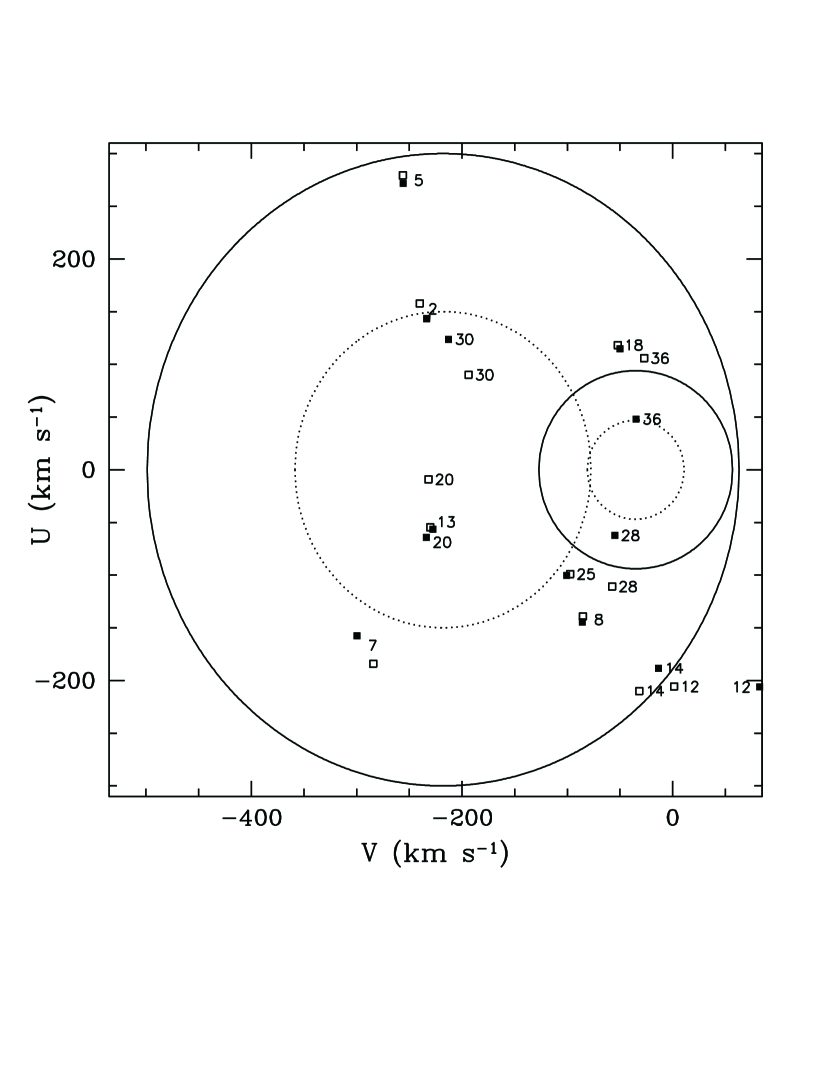
Figure 4: The effect of radial velocities on the $UV$-plane kinematics. We plot the original OHDHS positions of our radial velocity sample (open squares), and their positions in the $UV$ plane after the radial velocities have been take into account (filled squares). Numbers should help match the corresponding points.

For our radial velocity sample of OHDHS WDs we can calculate actual velocity components $U$, $V$ and $W$, and thus directly test and quantify the validity of $W=0$ assumption. In Figure 4 we plot as open squares the original OHDHS positions of 13 WDs with radial velocities, and as filled squares their positions when the radial velocities are take into account. To help match the corresponding points we put sequential numbers next to them. We see that the changes range from negligible to moderately high (point 12 = LHS 4033 moved by $81\,{\rm km}\,{\rm s}^{-1}$). On average, the points have moved by $29\,{\rm km}\,{\rm s}^{-1}$. What about the change in $UV$ velocity? First we see that as a result of radial velocity knowledge, two objects that were just outside of the $94\,{\rm km}\,{\rm s}^{-1}$ cut have moved inward. These two cases actually represent the largest changes ($-48$ and $-58\,{\rm km}\,{\rm s}^{-1}$), while the average change is just $-5\,{\rm km}\,{\rm s}^{-1}$. On average, each individual $UV$ velocity is smaller by 6% (with a scatter of 21%). Thus it seems that this is a modest effect, and that the use of $W=0$ assumption in the absence of radial velocities is appropriate for this sample. Note that in this comparison we kept the sky-projected (tangential) velocities the same, i.e., we used the original OHDHS values.

5.2 New distances and the $UV$-plane velocities

Newly determined distances will, through modified sky-projected velocities, directly affect the derived values of $U$ and $V$ velocity components. We already saw the result of this in §4.4, where the new distances produced 13 new cool WD candidates with potential halo kinematics. Also, in §4.3.4, we saw that there is a systematic trend affecting large distances more than the nearby ones. Since on average we expect high $UV$ values to belong to farther objects, we would expect that this trend will be reflected in the $UV$ plane. The revised proper motions will also be responsible for some change, albeit a very slight one.

In Figure 5 we show the new (filled squares), and the original (open squares; equivalent to OHDHS Figure 3) $UV$-plane positions of the 38 OHDHS WDs. In both cases the radial velocities are neglected, i.e., $W=0$. To avoid clutter, individual points are not labeled, yet we notice that the new $UV$ velocities tend to be higher, especially for already high values. The analysis shows that on average points have moved by $46\,{\rm km}\,{\rm s}^{-1}$, while the $UV$ velocity on average increased by $23\,{\rm km}\,{\rm s}^{-1}$ (with maximum change being $+171\,{\rm km}\,{\rm s}^{-1}$). Each individual $UV$ velocity is on average larger by 10% (with a scatter of 30%).

Thus, the net effect of radial velocities and new distance determinations is that the average $UV$ velocities are somewhat higher than the original ones.

5.3 Velocity component perpendicular to the Galactic plane

For our radial velocity subsample of 13 WDs we can determine true velocities in the direction perpendicular to the Galactic plane – the $W$ component. We plot the $W$ values in Figure 6 as a function of the $UV$ velocity. We have also added two WDs from the newly qualified cool WDs that have radial velocities measured by (Pauli et al., 2003) (open circles). Omitting the two WDs with $UV\leqslant 94\,{\rm km}\,{\rm s}^{-1}$, we find the $W$ dispersion of the LRIS sample to be $\sigma_{W}=59\,{\rm km}\,{\rm s}^{-1}$. Only one WD (LHS 4033, $V-I=0.06$) exceeds $100\,{\rm km}\,{\rm s}^{-1}$ – reaching $W=-153\,{\rm km}\,{\rm s}^{-1}$. Without it, we would have $\sigma_{W}=44\,{\rm km}\,{\rm s}^{-1}$. Actually, Dahn et al. (2004) are about to publish trigonometric parallax for this white dwarf. It turns out that LHS 4033 is very massive ($M=1.25M_{\odot}$), and thus some three times closer than estimated based on $0.6M_{\odot}$ CMR. This measurement also affects its surface gravity, producing much larger gravitational redshift than we assume for our WDs. Altogether, if one was to use this information a posteriori (which can be strongly argued against), we would get $\sigma_{W}=45\,{\rm km}\,{\rm s}^{-1}$. Anyhow, these values are in between the values usually derived for thick disk and spheroid (halo) populations, $35\,{\rm km}\,{\rm s}^{-1}$ and $94\,{\rm km}\,{\rm s}^{-1}$, respectively (Chiba & Beers, 2000). That the radial velocity sample probes mostly what appears to be a lower velocity (and younger?) population was already indicated in §4.1.3. Indeed, all but three of the radial velocity WDs are proper-motion limited. While one can formally calculate $\sigma_{U}$ and $\sigma_{V}$, they are meaningless because of the $UV$ selection that was applied to derive the sample in the first place. We defer a more thorough analysis of the kinematics and population analysis to a forthcoming paper.

5.4 Space density of white dwarfs

The derived space density, and thus the mass density, of OHDHS cool white dwarfs was their key result, and the one that stirred most controversy, since it is considerably higher than the expected stellar (as opposed to dark matter) halo WD density. Using OHDHS original data for 38 cool WDs, and applying the same $1/{\mathbf{V}}_{\rm max}$ technique, with a limiting magnitude of $R_{\rm 59F}^{\rm lim}=19.8$, one derives $n=1.4\times 10^{-4}\,{\rm pc}^{-3}$ (close to the value given by OHDHS of $1.8\times 10^{-4}\,{\rm pc}^{-3}$). Using a typical WD mass of $0.6M_{\odot}$, this corresponds to $\rho=8.3\times 10^{-5}\,{M_{\odot}}{\rm pc}^{-3}$, or some six times higher than the canonical value of stellar halo WD mass density of $\rho_{c}=1.3\times 10^{-5}\,{M_{\odot}}{\rm pc}^{-3}$ (Gould, Flynn, & Bahcall, 1998). (Note that this often quoted canonical value is somewhat of an educated guess, and not a real measurement (A. Gould, private communication 2003)).

What estimate of density would we get with our updated data? In our analysis we include all cool WD candidates from Table 4, using the radial velocity data where available. For completeness, we append this list with the remaining low-velocity WDs identified by OHDHS ($UV\leqslant 94\,{\rm km}\,{\rm s}^{-1}$). For them, we use listed SuperCOSMOS proper motions and do not check for the availability of radial velocities in the literature. Looking at the entire WD sample of 98 objects will allow us to characterize the density not just for a sample with a fixed $UV$ cut, but rather as a function of the $UV$-cutoff velocity.

Of 47 WDs with $UV>94\,{\rm km}\,{\rm s}^{-1}$ only 12 are magnitude-limited. All others, including all 51 WDs with $UV\leqslant 94\,{\rm km}\,{\rm s}^{-1}$ are proper-motion limited, that is, the maximum distance at which they could be detected is determined by the proper-motion lower limit of the survey ($330\,{\rm mas}\,{\rm yr}^{-1}$). For the magnitude limit we use $R_{\rm 59F}^{\rm lim}=19.8$ transformed for each object into a corresponding $V^{\rm lim}$ using the Equation 2.

If we restrict ourselves to the original $UV$-cut of $94\,{\rm km}\,{\rm s}^{-1}$, the 47 WDs that make this cut yield

$$n_{94}=1.72\times 10^{-4}\,{\rm pc}^{-3}$$ (12)

which is similar or slightly higher than the original estimate based on 38 WDs and $R_{\rm 59F}^{\rm lim}=19.8$. For this sample we have $\langle{\mathbf{V}}/{\mathbf{V}}_{\rm max}\rangle=0.51$, suggesting that $R_{\rm 59F}^{\rm lim}$ has an appropriate value.

How sensitive is this estimate on the choice of $UV$-cutoff velocity? In Figure 7 we plot cumulative number density starting from the highest $UV$ values (dotted line). However, since at higher $UV$ values we limit ourselves to yet smaller portion of the $UV$-plane, we need to correct it. We do it by finding (at each $UV$) a fraction of objects with Chiba & Beers (2000) halo kinematics that get excluded by different $UV$ cuts. (The correction factor is normalized to 1 for $UV=94\,{\rm km}\,{\rm s}^{-1}$, in order to make the results directly comparable to OHDHS who did not perform this correction. In any case, the actual correction at this velocity is very small).

The corrected densities are shown with a solid line. The lower panel monitors $\langle{\mathbf{V}}/{\mathbf{V}}_{\rm max}\rangle$ at each point, and appears consistent with 0.5 for the entire range of interest. The vertical thin line denotes the $94\,{\rm km}\,{\rm s}^{-1}$ limit. Inward of this limit we have a rise of density due to non-halo populations. Actually, we see that this rise begins inward of $UV\sim 150\,{\rm km}\,{\rm s}^{-1}$. Note that in the corrected plot, the density of objects with halo kinematics should be independent of the $UV$ cut. The corrected density at $UV=150\,{\rm km}\,{\rm s}^{-1}$ is

$$n_{150}=0.42\times 10^{-4}\,{\rm pc}^{-3},$$ (13)

corresponding to $1.9\,\rho_{c}$. The minimum value of the attained density is

$$n_{\rm min}=0.31\times 10^{-4}\,{\rm pc}^{-3},$$ (14)

at $UV\sim 190\,{\rm km}\,{\rm s}^{-1}$. This minimum value corresponds to $1.4\,\rho_{c}$ – within the uncertainty of the stellar halo WD density. Beyond $UV\sim 250\,{\rm km}\,{\rm s}^{-1}$, the density estimate rises again. It exceeds $n_{94}$ when $UV>400\,{\rm km}\,{\rm s}^{-1}$. However, in this range, the density is based on just 2–3 highest velocity objects with huge correction factors.

6 Conclusions

We obtain precise radial velocities for the majority of OHDHS WDs with ${\rm H}\alpha\,$lines. This makes it possible to measure more precisely the $U$ and $V$ components of the velocity, and also allows the $W$ component to be derived. We show that the radial velocities do not affect significantly the way in which OHDHS selected their cool WD candidates. Our $W$-velocity dispersion lies between the typical thick disk and halo values, an indication of a mixed sample.

Also, our new CCD photometry, and the recalibration of OHDHS SuperCOSMOS plate photometry, allow for more robust distance estimates.

Finally, with the new dataset, and applying the same methods of analysis as in OHDHS, we confirm the densities of cool white dwarfs that they derived. However, many times lower densities (consistent with the stellar halo) are found if one adopts higher $UV$-cutoff velocities. This new set of data facilitates a more sophisticated analysis, which we plan to present in a forthcoming paper.

Figure 1: Kinematical selection effects of the radial velocity subsample. The two curves shows the straight (solid) and the weighted (dashed) average $UV$-velocity ($UV\equiv\sqrt{U^{2}+(V+35\,{\rm km}\,{\rm s}^{-1})^{2}}$) of random subsamples of 13 white dwarfs (out of 38 OHDHS cool white dwarfs). Compared to these distributions are the actual (straight and weighted) $UV$-velocity averages of our radial velocity subsample, shown with arrows.

Figure 2: $B-V$ vs. $V-I$ color-color diagram of OHDHS cool white dwarfs with CCD photometry. Filled circles are white dwarfs exhibiting ${\rm H}\alpha\,$line (DA type). The solid and the dashed tracks correspond to theoretical colors for $g=8$ white dwarfs with pure hydrogen and pure helium atmospheres, respectively. The models cover 4000–12,000 K temperature range, with triangles marking every 1000 K. Labeled objects are discussed in the text.

Figure 3: $V-J$ vs. $J-H$ color-color diagram of OHDHS cool white dwarfs present in 2MASS All-Sky Survey. See Figure 2 for legend. Tracks terminate at 10,000 K.

Figure 5: The effect of recalibrated distances on the $UV$ velocities. Original velocities of 38 OHDHS cool white dwarfs are shown as open squares (corresponding to their Figure 3), while values obtained with new distances (and proper motions) are shown as filled squares.

Figure 6: Component of motion perpendicular to the Galactic plane. $W$ velocities of 13 OHDHS white dwarfs with radial velocities measured by us are shown as filled circles. Two open circles come from the “additional” cool white dwarf candidates, and were measured by Pauli et al. (2003). Vertical line represents the $UV=94\,{\rm km}\,{\rm s}^{-1}$ cut.

Figure 7: Number density of OHDHS white dwarfs as a function of $UV$-cut velocity. In the upper panel we show the corrected (solid line) and the uncorrected (dotted line) cumulative density of all 98 white dwarfs observed by OHDHS (summing from the high-velocity end). The corrected line takes into account that at high $UV$ values we sample a smaller part of the $UV$ plane. Vertical line represents the $UV=94\,{\rm km}\,{\rm s}^{-1}$ cut. In the lower panel we monitor average $\langle{\mathbf{V}}/{\mathbf{V}}_{\rm max}\rangle$ as we move towards the lower $UV$ velocities. Note that beyond $\sim 300\,{\rm km}\,{\rm s}^{-1}$ we only have a couple of objects.

Table 1: Observed WDs and their radial velocities.

No.	Name	$v^{\rm obs}_{\rm rad}$ (${\rm km}\,{\rm s}^{-1}$)
2	WD0153-014	$-50\pm 7$
5	LHS 147	$-15\pm 7$
7	WD0135-039	$-28\pm 7$
8	LHS 4042	$-24\pm 7$
9	WD2356-209	$\cdots$
10	WD0227-444	$\cdots$
12	LHS 4033	$206\pm 7$
13	LP 586-51	$-22\pm 7$
14	WD2242-197	$-8\pm 7$
15	WD0205-053	$\cdots$
17	WD0125-043	$\cdots$
18	WD2346-478	$75\pm 7$
20	WD0300-044	$141\pm 13$
21	WD0123-278	$\cdots$
24	LHS 1402	$\cdots$
25	LHS 1274	$81\pm 7$
27	WD0044-284	$\cdots$
28	WD2214-390	$50\pm 7$
30	LP 588-37	$-127\pm 7$
32	WD0045-061	$\cdots$
33	WD0225-326	$\cdots$
35	WD0117-268	$\cdots$
36	LP 651-74	$74\pm 7$

Table 2: Johnson-Cousins CCD photometry

No.	Name	$B$	$V$	$R$	$I$	$n_{\rm obs}$
2	WD0153-014	$\cdots$	$18.646\pm 0.020$	$\cdots$	$18.415\pm 0.034$	0202
3	LHS 542	$19.473\pm 0.053$	$18.221\pm 0.023$	$17.545\pm 0.025$	$16.926\pm 0.028$	2321
5	LHS 147	$17.985\pm 0.018$	$17.615\pm 0.011$	$\cdots$	$17.169\pm 0.016$	3202
6	WD2326-272	$21.027\pm 0.165$	$19.922\pm 0.051$	$\cdots$	$19.095\pm 0.051$	2202
7	WD0135-039	$\cdots$	$19.644\pm 0.048$	$\cdots$	$19.083\pm 0.065$	0402
9	WD2356-209	$21.206\pm 0.109$	$20.850\pm 0.075$	$\cdots$	$18.878\pm 0.033$	2404
12	LHS 4033	$17.162\pm 0.020$	$16.992\pm 0.017$	$16.987\pm 0.030$	$16.936\pm 0.036$	3222
13	LP 586-51	$18.318\pm 0.039$	$18.185\pm 0.022$	$18.141\pm 0.044$	$18.096\pm 0.039$	1212
14	WD2242-197	$20.504\pm 0.098$	$19.659\pm 0.045$	$\cdots$	$18.861\pm 0.074$	1201
15	WD0205-053	$\cdots$	$18.898\pm 0.145$	$\cdots$	$17.257\pm 0.024$	0101
17	WD0125-043	$\cdots$	$19.820\pm 0.076$	$\cdots$	$18.911\pm 0.054$	0202
20	WD0300-044	$20.782\pm 0.266$	$19.862\pm 0.049$	$\cdots$	$19.301\pm 0.051$	1404
24	LHS 1402	$\cdots$	$18.050\pm 0.014$	$\cdots$	$18.422\pm 0.027$	0205
27	WD0044-284	$\cdots$	$20.022\pm 0.060$	$\cdots$	$18.713\pm 0.039$	0402
30	LP 588-37	$\cdots$	$18.496\pm 0.024$	$\cdots$	$18.365\pm 0.039$	0303
32	WD0045-061	$\cdots$	$18.203\pm 0.015$	$\cdots$	$17.219\pm 0.019$	0302
35	WD0117-268	$\cdots$	$19.057\pm 0.049$	$\cdots$	$17.944\pm 0.030$	0303
36	LP 651-74	$18.033\pm 0.021$	$17.342\pm 0.011$	$\cdots$	$16.568\pm 0.015$	2202

Table 3: Comparison with the published photometry

Name	$B$	$V$	$R$	$I$	Reference
LHS 542	19.23	18.15	17.53	16.99	Bergeron, Leggett, & Ruiz (2001)
	19.49	18.25	$\cdots$	$\cdots$	Liebert, Dahn, & Monet (1988)
	19.47	18.22	17.55	16.93	This work
LHS 147	17.97	17.62	17.38	17.16	Bergeron, Ruiz, & Leggett (1997)
	18.09	17.66	$\cdots$	$\cdots$	Liebert, Dahn, & Monet (1988)
	17.94	17.57	$\cdots$	$\cdots$	Eggen & Sandage (1967)
	17.99	17.62	$\cdots$	17.17	This work

Table 4: The new dataset – relevant data on cool white dwarfs

No.	Name	R.A.	Dec.	$\mu_{\alpha}$	$\mu_{\delta}$	$\sigma(\mu_{\alpha})$	$\sigma(\mu_{\delta})$	Flag A	$V$	$V-I$	Flag P	$d$	$\sigma_{d}$	Flag C	$v_{\rm rad}$	$\sigma(v_{\rm rad})$
		(deg)	(deg)	${\rm mas}\,{\rm yr}^{-1}$	${\rm mas}\,{\rm yr}^{-1}$	${\rm mas}\,{\rm yr}^{-1}$	${\rm mas}\,{\rm yr}^{-1}$		mag	mag		pc	pc		${\rm km}\,{\rm s}^{-1}$	${\rm km}\,{\rm s}^{-1}$
1	F351-50	11.33178	$-$33.49130	1860	$-$1486	51	10	U	19.37	1.54	O	40	10	He	$\cdots$	$\cdots$
2	WD0153-014	28.46448	$-$1.39468	64	$-$398	4	6	U	18.65	0.23	S	170	36	H	$-$79	9
3	LHS 542	349.78956	$-$6.21383	$-$618	$-$1584	1	5	U	18.22	1.29	S	31	7	He	$\cdots$	$\cdots$
4	WD0351-564	57.78907	$-$56.45198	265	$-$1052	20	19	O	20.96	1.49	O	88	22	He	$\cdots$	$\cdots$
5	LHS 147	27.03805	$-$17.20401	$-$120	$-$1106	7	6	U	17.61	0.45	S	75	15	H	$-$44	9
6	WD2326-272	351.54458	$-$27.24632	576	$-$104	4	9	U	19.92	0.83	S	112	27	He	$\cdots$	$\cdots$
7	WD0135-039	23.89029	$-$3.95502	454	$-$186	7	6	U	19.64	0.56	S	160	38	H	$-$57	9
8	LHS 4042	358.64586	$-$32.35540	422	$-$46	1	10	U	17.41	0.18	O	105	25	H	$-$52	9
9	WD2356-209	359.18788	$-$20.91370	$-$329	$-$211	32	20	O	20.85	1.97	S	74	34	sp	$\cdots$	$\cdots$
10	WD0227-444	36.87318	$-$44.38573	268	$-$217	12	18	O	19.82	1.06	O	83	22	He?	$\cdots$	$\cdots$
11	J0014-3937	3.44777	$-$39.62331	$-$226	$-$714	17	2	U	18.70	1.25	O	40	10	He	$\cdots$	$\cdots$
12	LHS 4033	358.13289	$-$2.88647	614	324	10	8	U	16.99	0.06	S	105	22	H	178	9
13	LP 586-51	15.53001	$-$0.54986	342	$-$122	3	3	U	18.19	0.09	S	172	37	H	$-$51	9
14	WD2242-197	340.43428	$-$19.67841	346	62	4	4	U	19.66	0.80	S	111	27	H	$-$36	9
15	WD0205-053	31.29830	$-$5.29836	956	400	3	6	U	18.90	1.64	S	29	8	He	$\cdots$	$\cdots$
16	WD0100-645	15.20987	$-$64.48649	516	190	5	0	U	17.58	0.58	O	60	14	H	$\cdots$	$\cdots$
17	WD0125-043	21.27431	$-$4.28424	250	$-$44	6	4	U	19.82	0.91	S	98	25	He	$\cdots$	$\cdots$
18	WD2346-478	356.51213	$-$47.85060	$-$270	$-$454	5	3	U	17.95	0.83	O	48	11	H	47	10
19	LHS 1447	42.05496	$-$30.02575	436	322	0	6	U	18.43	0.44	O	106	25	He	$\cdots$	$\cdots$
20	WD0300-044	45.09852	$-$4.42355	272	$-$280	17	19	O	19.86	0.56	S	177	41	H	112	15
21	WD0123-278	20.76574	$-$27.80398	342	124	5	16	U	20.29	1.29	O	80	26	He?	$\cdots$	$\cdots$
22	WD2259-465	344.77772	$-$46.46632	404	$-$158	4	7	U	19.71	1.26	O	64	20	He?	$\cdots$	$\cdots$
23	WD0340-330	55.03620	$-$33.01671	494	$-$330	3	5	U	19.94	1.17	O	77	22	He?	$\cdots$	$\cdots$
24	LHS 1402	36.13432	$-$28.91646	492	$-$30	3	2	U	18.05	$-$0.37	S	21	5	sp	$\cdots$	$\cdots$
25	LHS 1274	24.80995	$-$33.81756	580	$-$24	3	11	U	17.34	0.49	O	62	15	H	52	9
26	WD0214-419	33.56203	$-$41.85251	320	$-$96	18	19	O	20.08	0.98	O	102	25	He	$\cdots$	$\cdots$
27	WD0044-284	11.00892	$-$28.40313	$-$78	$-$360	13	3	U	20.02	1.31	S	69	23	He?	$\cdots$	$\cdots$
28	WD2214-390	333.64480	$-$38.98522	1006	$-$360	2	8	U	16.14	0.67	O	27	6	H	21	9
29	WD2324-595	351.04227	$-$59.46895	124	$-$576	5	7	U	16.90	0.14	O	88	21	H	$\cdots$	$\cdots$
30	LP 588-37	25.58649	$-$1.39757	108	$-$344	1	7	U	18.50	0.13	S	186	40	H	$-$155	9
31	WD0345-362	56.38631	$-$36.18446	142	$-$588	18	67	U	20.40	1.45	O	71	17	He	$\cdots$	$\cdots$
32	WD0045-061	11.27623	$-$6.13876	104	$-$676	3	3	U	18.20	0.98	S	43	10	He	$\cdots$	$\cdots$
33	WD0225-326	36.36950	$-$32.63163	310	160	36	4	U	18.61	0.40	O	118	28	He	$\cdots$	$\cdots$
34	WD2348-548	357.19527	$-$54.76280	364	$-$96	22	32	U	19.21	0.98	O	69	17	He	$\cdots$	$\cdots$
35	WD0117-268	19.46521	$-$26.81428	476	42	3	3	U	19.06	1.11	S	55	15	He?	$\cdots$	$\cdots$
36	LP 651-74	46.80880	$-$7.24976	$-$193	$-$436	11	10	O	17.34	0.77	S	40	8	H	45	9
37	WD0135-546	23.91108	$-$54.59108	660	108	17	3	U	18.91	1.13	O	51	14	He?	$\cdots$	$\cdots$
38	WD0100-567	15.17948	$-$56.77684	293	293	6	8	O	17.44	0.60	O	55	13	H	$\cdots$	$\cdots$
A1	WD2221-402	335.46833	$-$40.19267	316	$-$238	17	0	U	19.81	1.09	O	80	20	He	$\cdots$	$\cdots$
A2	WD2342-225	355.56890	$-$22.45330	312	90	6	2	U	19.41	0.82	O	90	22	He	$\cdots$	$\cdots$
A3	WD0007-031	1.77802	$-$3.11857	224	$-$390	3	4	U	18.44	0.79	O	64	15	H?	$\cdots$	$\cdots$
A4	WD2236-168	339.06532	$-$16.79833	318	$-$60	3	6	U	18.48	0.75	O	69	17	He	$\cdots$	$\cdots$
A5	WD2234-408	338.72467	$-$40.75506	287	$-$249	17	14	O	17.72	0.47	O	76	18	H	$\cdots$	$\cdots$
A6	LHS 1044	3.55330	$-$13.18362	$-$554	$-$708	2	2	U	15.78	0.68	O	22	6	H	$\cdots$	$\cdots$
A7	J0424-4551	65.99036	$-$45.84513	$-$100	$-$532	15	1	U	16.85	0.73	O	34	8	H	$\cdots$	$\cdots$
A8	LHS 3917	348.82831	$-$2.16120	584	192	3	1	U	16.48	0.50	O	41	10	He	$\cdots$	$\cdots$
A9	LHS 4041	358.57837	$-$36.56524	26	$-$664	1	2	U	15.46	$-$0.02	O	59	14	H	$-$27	3
A10	JL 193	7.85905	$-$44.63682	342	28	13	10	U	16.89	0.11	O	91	24	He	$\cdots$	$\cdots$
A11	LP 880-451	1.78131	$-$31.22642	336	$-$124	3	6	U	16.47	$-$0.12	O	108	26	He	$\cdots$	$\cdots$
A12	LHS 1076	6.66973	$-$55.41222	$-$294	$-$450	5	10	U	15.16	0.23	O	34	9	H	$\cdots$	$\cdots$
A13	WD0252-350	43.65459	$-$34.83158	44	$-$328	2	3	U	15.79	$-$0.05	O	71	17	H	86	2

Note. — Objects below the line are the new cool WD candidates, coming from OHDHS sample, but not listed in OHDHS paper. Coordinates are given for epoch and equinox 2000. Radial velocities are corrected for gravitational redshift and come from this work, except for A9 and A13 (Pauli et al., 2003).

References

- Afonso et al. (2003) Afonso, C. et al. 2003, A&A, 400, 951
- Alcock et al. (2000) Alcock, C. et al. 2000, ApJ, 542, 281
- Bergeron (2003) Bergeron, P. 2003, ApJ, 586, 201
- Bergeron & Leggett (2002) Bergeron, P. & Leggett, S. K. 2002, ApJ, 580, 1070
- Bergeron, Leggett, & Ruiz (2001) Bergeron, P., Leggett, S. K., & Ruiz, M. T. 2001, ApJS, 133, 413
- Bergeron, Ruiz, & Leggett (1997) Bergeron, P., Ruiz, M. T., & Leggett, S. K. 1997, ApJS, 108, 339
- Bergeron et al. (1994) Bergeron, P., Ruiz, M., Leggett, S. K., Saumon, D., & Wesemael, F. 1994, ApJ, 423, 456
- Bergeron, Saumon, & Wesemael (1995) Bergeron, P., Saumon, D., & Wesemael, F. 1995, ApJ, 443, 764
- Bergeron, Wesemael, & Beauchamp (1995) Bergeron, P., Wesemael, F., & Beauchamp, A. 1995, PASP, 107, 1047
- Bessell (1986) Bessell, M. S. 1986, PASP, 98, 1303
- Blair & Gilmore (1982) Blair, M. & Gilmore, G. 1982, PASP, 94, 742
- Chiba & Beers (2000) Chiba, M. & Beers, T. C. 2000, AJ, 119, 2843
- Dahn et al. (2004) Dahn, C. C. et al. 2004, in prep.
- Digby et al. (2003) Digby, A. P., Hambly, N. C., Cooke, J. A., Reid, I. N., & Cannon, R. D. 2003, astro-ph/0304056.
- Eggen & Sandage (1967) Eggen, O. J. & Sandage, A. 1967, ApJ, 148, 911
- Freese, Fields, & Graff (2000) Freese, K., Fields, B., & Graff, D. 2000, The First Stars. Proceedings of the MPA/ESO Workshop, Garching, Germany, 4-6 August 1999. Achim Weiss, Tom G. Abel, Vanessa Hill (eds.). Springer, p.18, 18 (also available as astro-ph/0002058)
- Garnavich et al. (1998) Garnavich, P. M. et al. 1998, ApJ, 493, L53
- Gould (2003) Gould, A. 2003, AJ, 126, 472
- Gould, Flynn, & Bahcall (1998) Gould, A., Flynn, C., & Bahcall, J. N. 1998, ApJ, 503, 798
- Hambly, Irwin, & MacGillivray (2001) Hambly, N. C., Irwin, M. J., & MacGillivray, H. T. 2001, MNRAS, 326, 1295
- Hambly, Davenhall, Irwin, & MacGillivray (2001) Hambly, N. C., Davenhall, A. C., Irwin, M. J., & MacGillivray, H. T. 2001, MNRAS, 326, 1315
- Hambly et al. (2001) Hambly, N. C. et al. 2001, MNRAS, 326, 1279
- Hansen (1998) Hansen, B. M. S. 1998, Nature, 394, 860
- Hansen & Liebert (2003) Hansen, B. M. S., & Liebert, J., 2003, ARA&A, in press
- Harris et al. (2003) Harris, H. C. et al. 2003, AJ, 126, 1023
- Lasserre et al. (2000) Lasserre, T. et al. 2000, A&A, 355, L39
- Liebert, Dahn, & Monet (1988) Liebert, J., Dahn, C. C., & Monet, D. G. 1988, ApJ, 332, 891
- Monet et al. (2003) Monet, D. G. et al. 2003, AJ, 125, 984
- Oke et al. (1995) Oke, J. B. et al. 1995, PASP, 107, 375
- Oppenheimer et al. (2001) Oppenheimer, B. R., Hambly, N. C., Digby, A. P., Hodgkin, S. T., & Saumon, D. 2001, Science, 292, 698 (OHDHS)
- Paczyński (1986) Paczyński, B. 1986, ApJ, 304, 1
- Pauli et al. (2003) Pauli, E.-M., Napiwotzki, R., Altmann, M., Heber, U., Odenkirchen, M., & Kerber, F. 2003, A&A, 400, 877
- Reid (1996) Reid, I. N. 1996, AJ, 111, 2000
- Reid, Sahu, & Hawley (2001) Reid, I. N., Sahu, K. C., & Hawley, S. L. 2001, ApJ, 559, 942
- Riess et al. (1998) Riess, A. G. et al. 1998, AJ, 116, 1009
- Sahu (1994) Sahu, K. C. 1994, Nature, 370, 275
- Saumon et al. (1994) Saumon, D., Bergeron, P., Lunine, J. I., Hubbard, W. B., & Burrows, A. 1994, ApJ, 424, 333
- Saumon & Jacobson (1999) Saumon, D. & Jacobson, S. B. 1999, ApJ, 511, L107
- Scholz et al. (2000) Scholz, R.-D., Irwin, M., Ibata, R., Jahreiß, H., & Malkov, O. Y. 2000, A&A, 353, 958
- Silvestri et al. (2001) Silvestri, N. M., Oswalt, T. D., Wood, M. A., Smith, J. A., Reid, I. N., & Sion, E. M. 2001, AJ, 121, 503
- Silvestri, Oswalt, & Hawley (2002) Silvestri, N. M., Oswalt, T. D., & Hawley, S. L. 2002, AJ, 124, 1118