The cluster environments of radio-loud quasars at $0.6<z<1.1$

Abstract

We have carried out multicolour imaging of a complete sample of radio-loud quasars at $0.6<z<1.1$ and find groups or clusters of galaxies in the fields of at least 8 and possibly 13 of the 21 sources. There is no evidence for an evolution in the richness of the environments of radio-loud quasars from other low-redshift studies to $z\gtrsim 0.9$. The quasars associated with groups and clusters in our sample do not necessarily reside in the centre of the galaxy distribution which rarely displays a spherical geometry. Clustering is preferentially associated with small or asymmetric steep-spectrum radio sources. The quasars with the largest projected angular size are, in nearly all cases, found in non-clustered environments. Radio-based selection (including source size) of high-redshift groups and clusters can be a very efficient method of detecting rich environments at these redshifts.

We find that in optical searches for galaxy overdensities above $z\sim 0.6$ multiple filters must be used. If the single-filter counting statistics used by groups at lower redshift are applied to our data, uncertainties are too large to make accurate quantifications of cluster richness. This means that genuine clustering of galaxies about quasars will be missed and, in $\sim 10\%$ of cases, putative clusters turn out to be false detections. The statistics are further diluted by the fact that galaxy overdensities are generally not centred on the quasar.

1 Introduction

Groups and clusters of galaxies at high redshift are key targets for studying the evolution of galaxies and large-scale structure. They provide insight into the star formation history of the earliest galaxies (eg: Barger et al. 1996; Poggianti et al. 1996; Balogh et al. 1997; Kodama & Bower 2001), as well as being powerful probes of the growth of structure [Dressler 1980, van Dokkum & Franx 2001]. In addition, they are observational points of reference for theoretical simulations of structure formation which can provide insight into the cosmological parameters (eg: Gross et al. 1998; Jenkins et al. 1998; Yoshida et al. 2001). However, finding large numbers of clustered systems above $z\sim 0.5$ has proved difficult and time consuming. The main methods focus on searching for large-scale or extended structure over wide areas. One such technique has looked for X-ray emission from hot intracluster gas (eg: Gioia & Luppino 1994; Rosati et al. 1998), which is biassed toward finding the most massive and/or merging systems. Other efforts have concentrated on finding overdensities of objects in deep optical images taken in a single filter (eg: Couch et al. 1991; Lidman & Petersen 1996; Postman et al. 1996; Olsen et al. 1999a). Optical identification of clusters on the basis of numerical/statistical overdensities of faint galaxies becomes increasingly problematic at higher redshift ($z>0.5$) due to the variance in the faint number counts on the scale length of clusters. More recent surveys have attempted to mitigate this latter problem by using multiple filters to preselect objects with the same colours , and hence probable redshift (eg: Olsen et al. 1999b; Gladders & Yee 2000; Martini 2000; Drory et al. 2001). However, all blank-field surveys are still inefficient in terms of clusters found per unit observing time.

It has been known for some time that groups and clusters of galaxies share a close relationship with active galactic nuclei (AGN). AGN at low redshift have been shown to exist in environments of above average galactic density [Seldner & Peebles 1978, Longair & Seldner 1979, Steiner, Grindlay & Maccacaro 1982, Yee & Green 1984, Yee & Green 1987] and studies extending these observations to higher redshift have shown that at $z>0.3$ high-luminosity AGN reside in the richest clusters [Ellingson et al. 1991, Hill & Lilly 1991]. Detailed knowledge of an AGN environment can provide tests of proposed unification schemes [Wurtz et al. 1997], as well as shedding light on the luminosity evolution of AGN [Ellingson et al. 1991]. Furthermore, the current co-moving space density of Abell class 0 clusters at low redshift is similar to that of powerful radio sources at $z\sim 2-3$ [McLure & Dunlop 2001]. The implication is that all present day clusters hosted a powerful radio source at sometime in the past (see also Bremer et al. 1992). We exploit this close relationship in order to create a sample of distant groups and clusters of galaxies with well understood biases by searching for overdensities of galaxies associated with radio-loud quasars (RLQs).

Previous studies of clustering of galaxies around AGN have endeavoured to quantify the clustering with reference to the statistical overdensity of objects found within a certain radius (usually 0.5 Mpc) of the AGN in a single filter (eg: Yee & Green 1987; Hutchings 1995; Hall, Green & Cohen 1998; Wold et al. 2000). However, a more robust strategy, which we follow, is to identify high-redshift cluster members from their optical and near-infrared (NIR) colours. This exploits the narrow colour dispersion amongst the passively-evolving elliptical galaxy population (the red sequence) making up the cores of clusters [Baum 1959, Bower, Lucey & Ellis 1992, Stanford et al. 1998]. A similar method is used in the wide-field cluster searches of Gladders & Yee (2000) who claim that the red sequence is present as a visible indicator of a cluster core out to $z>1.2$. Our method has the advantage of being able to select the redshift of interest and hence choose filters to pick out the characteristic cluster galaxies at that redshift. Core cluster members above $z\sim 0.5$ are readily identifiable by using a combination of optical and NIR filters. Optical filters can be used to straddle the prominent 4000Å break of passively-evolving elliptical galaxies, thus maximising the contrast for these objects. Using $J$ and $K$ filters with one optical filter such as $R$ or $I$ separates high-redshift ellipticals from spirals or M-stars and brown dwarfs, as shown in Pozzetti & Manucci (2000) and Figure 1.

Figure 1: The evolution of $R-K^{\prime}$ vs. $J-K^{\prime}$ colours for two galaxies at redshifts 0 to 2. Thick line: An elliptical formed from a single burst of star formation at $z=5$. Dotted line: A spiral formed at the same $z$. Indicated are the redshifts at points relevant to our sample. The plots were constructed using the synthetic spectra of Fioc & Rocca-Volmerange (1997).

This paper presents results of deep multicolour imaging of a representative sample of 21 radio-loud quasars with $0.6<z<1.1$. The goal is to identify evolved cluster cores by finding excesses of passively-evolving elliptical galaxies in the quasar fields. Preliminary results for two fields have been published in Baker et al. (2001) and Bremer, Baker & Lehnert (2002). Here, as in these previous papers, we analyse quasar fields individually and report the identification of clustering in the fields of up to 13 of the 21 RLQs. However, the power of a complete redshift-limited target sample is that we can extend the analysis to the sample as a whole. As well as discovering high-redshift groups and clusters of galaxies, we can correlate the existence of clustering with the properties of the RLQs. A detailed analysis of how the radio properties of the sources depend on environment, incorporating theoretical considerations of the growth of FRII radio lobes in clustered environments will be published in a subsequent paper (Barr, Bremer & Baker 2003, in preparation). In the present analysis, we concentrate on detecting clustered systems about AGN and the optical-NIR properties of their core galaxy population.

Details of the target sample and observations are given in Section 2. Single filter statistics are measured and compared with other studies in Section 3. Multicolour analysis of all the fields are presented in Section 4. A discussion of the relative merits of cluster quantification methods is given in Section 5, along with the cluster characteristics of the RLQ sample. For comparison with previous studies we adopt a $H_{0}=50$ km s^-1 Mpc^-1, $\Omega_{m}=1$, $\Lambda=0$ cosmology.

2 Observations and Data reduction

2.1 The Sample

The quasars used for this study are a redshift-limited subsample of the Molonglo Quasar Sample (MQS; Kapahi et al. 1998) of low-frequency-selected radio-loud quasars. This is a highly complete ($>97\%$) sample of 111 RLQs with $S_{408}>0.95$ Jy in the declination range $-30^{\circ}>\delta>-20^{\circ}$, and Galactic latitude $|b|>20^{\circ}$ (excluding the R.A. ranges $06^{\mathrm{h}}00^{\mathrm{m}}$ – $09^{\mathrm{h}}00^{\mathrm{m}}$ and $14^{\mathrm{h}}03^{\mathrm{m}}$ – $20^{\mathrm{h}}20^{\mathrm{m}}$). These objects are on average five times less powerful and so more numerous at a given redshift than 3CR sources [Laing, Riley & Longair 1983]. The MQS therefore probes a more representative subset of the RLQ population than do 3C quasars.

The sample presented in this paper is well suited to a study of radio-loud quasar environments. Its low-frequency (408 MHz) radio selection effectively picks out the steep-spectrum lobe contribution which results in a sample with few beamed objects, ie: those which may be of intrinsically lower luminosity but have Doppler boosted emission due to the orientation of the radio jet to the line of sight. Excluding sources with highly beamed emission is important as it gives us a good measure of the intrinsic power of the radio source. This is vital when attempting to correlate radio and environmental properties. Selecting on radio luminosity also prevents the omission of optically obscured quasars. Additionally, the MQS has the advantage of having been studied in a number of wavelength regimes (eg: Baker, Hunstead & Brinkmann 1995; Baker 1997; Ishwara-Chandra 1998; Kapahi et al. 1998; Baker et al. 1999; Ishwara-Chandra et al. 2001; Baker et al. 2002).

We have observed an RA- and redshift-limited subset of the MQS. Within the range $0^{\mathrm{h}}0^{\mathrm{m}}$$<\mathrm{RA}<$$14^{\mathrm{h}}0^{\mathrm{m}}$ there are 30 MQS objects which have $0.6<z<1.1$; we have data for 21 of these. The other nine sources were randomly excluded due to observing time restrictions. No quasars were excluded based on optical or radio criteria. The RLQs in this paper can therefore be thought of as a representative sample.

2.2 Optical images

Table 1: Summary of optical and NIR observing runs for the sample.

Run	Date	Telescope	Instrument	Pixel Scale	Field of View	Filters	Average Seeing
A	1996 Feb 14-16	ESO 2.2m	IRAC2B	$0^{\prime\prime}\!\!.51$	$2^{\prime}\!\!.17$ $\times$ $2^{\prime}\!\!.17$	$J$,$K^{\prime}$	$0^{\prime\prime}\!\!.8$
B	1996 Mar 19-21	CTIO 4m	PFCCD	$0^{\prime\prime}\!\!.16$	$5^{\prime}\!\!.4$ $\times$ $5^{\prime}\!\!.4$	$B$,$I$	$0^{\prime\prime}\!\!.5$
C	1997 Mar 12-15	ESO 3.6m	EFOSC	$0^{\prime\prime}\!\!.61$	$5^{\prime}\!\!.2$ $\times$ $5^{\prime}\!\!.2$	$V$,$R$,$I$,$z$	$0^{\prime\prime}\!\!.7$
D	1997 Mar 17-22	ESO 2.2m	IRAC2B	$0^{\prime\prime}\!\!.51$	$2^{\prime}\!\!.17$ $\times$ $2^{\prime}\!\!.17$	$J$,$K^{\prime}$	$1^{\prime\prime}\!\!.1$
E	1998 Feb 14-16	CTIO 4m	CIRIM	$0^{\prime\prime}\!\!.22$	$0^{\prime}\!\!.9$ $\times$ $0^{\prime}\!\!.9$	$H$	$0^{\prime\prime}\!\!.7$
F	1998 Mar 31-Apr 1	ESO 3.6m	EFOSC2	$0^{\prime\prime}\!\!.30$	$5^{\prime}\!\!.2$ $\times$ $5^{\prime}\!\!.2$	$R$,$I$	$0^{\prime\prime}\!\!.8$
G	1999 Sep 9	AAT 3.9m	Taurus	$0^{\prime\prime}\!\!.37$	$9^{\prime}\!\!.8$ diameter	$V$,$R$,$I$	$1^{\prime\prime}\!\!.5$
H	2000 Apr 11	AAT 3.9m	Taurus	$0^{\prime\prime}\!\!.37$	$9^{\prime}\!\!.8$ diameter	$V$,$R$,$I$	$2^{\prime\prime}\!\!.0$

Optical multicolour imaging of the fields was carried out in four separate runs using the PFCCD on the CTIO 4m Blanco telescope, EFOSC and EFOSC2 on the ESO 3.6m at La Silla and Taurus on the AAT. The field of view was $\sim 5^{\prime}$ for the CTIO and ESO runs and $9^{\prime}\!\!.8$ for the AAT data. Pixel scales ranged from $0^{\prime\prime}\!\!.16$ for PFCCD to $0^{\prime\prime}\!\!.61$ on EFOSC. Seeing varied between $0^{\prime\prime}\!\!.5$ and $2^{\prime\prime}\!\!.0$. The observing setup and conditions for all runs are detailed in Table 1.

The quasar fields were observed in two or more filters, selected from $B$, $V$, $R$, $I$ and Gunn $z$ according to the redshift of the target. The filters were chosen to straddle the 4000Å break and thus maximise the contrast for early type galaxies. Observations of each field in each filter were made up of 2 or 3 integrations dithered by $\sim 10^{\prime\prime}$ with respect to each other to facilitate cosmic ray rejection. Total integration times were typically 30 minutes to 1 hour per filter. Landolt photometric standards [Landolt 1992] were observed on 2–3 occasions on each night. Full details of the filters and exposure times used are given in Table 2.

Table 2: Summary of observations for the sample. For each object exposure times in seconds are on the upper row and the completeness limit in magnitudes is on the lower row.

MRC quasar		Optical							NIR
		Run(s)	$B$	$V$	$R$	$I$	$z$		Run(s)	$J$	$H$	$K^{\prime}$
B0030–220		G		1800		1800
				24.0		22.5
B0058–229		G		1800		1800
				23.0		21.5
B0209–237		G		1800		1800
				23.5		21.5
B0346–279		C			1800		1800		A	3600		3600
					23.5		22.0			20.5		19.0
B0450–221		C		1800		3600			A	3600		3600
				24.5		23.5				20.0		18.5
B0941–200		H		900	900	900			A,E	2400	3500	4020
				23.5	22.5	21.5				20.0	21.0	17.5
B1006–299		B,C	1800		1800	1800	6300		A	2400		3600
			24.0		24.0	22.5	22.5			19.5		18.5
B1055–242		C			3000		3600		D	4800
					24.0		22.5			20.5
B1121–238		C		900	600	900			D	1600		1800
				24.5	24.0	22.5				20.0		18.5
B1202–262		F			1800	1800
					25.0	23.5
B1208–277		C		1800		1800			A	3720		3000
				24.5		23.0				20.0		18.5
B1217–209		F			1800	1200
					24.5	24.0
B1222–293		F			1800	1800
					25.0	24.0
B1224–262		C		1800	900	1800			D	3200		1800
				24.5	24.0	23.0				20.0		18.5
B1226–297		F			1800	1800
					24.5	23.5
B1247–290		C		900	600	1800			D			2400
				24.5	24.0	23.0						17.5
B1301–251		B,C	1800	1800		900	1800		E		3600
			24.5	24.5		22.0	22.5				22.0
B1303–250		F			1200	600
					24.5	23.0
B1349–265		B,C	1800	1800		1800			D,E	11200	3150
			24.0	24.5		22.0				21.5	21.0
B1355–236		B,C	1800		600	1200
			24.0		24.0	22.0
B1359–281		B	1800			1200
			24.0			22.0

The data were bias subtracted and flat-fielded in a standard fashion using programs written in IDL. The flat-fielding was accomplished by using twilight sky flats or median-summed images of the science frames. Images in each filter were registered and co-added, rejecting cosmic rays. All apart from the $z$-band frames were photometrically calibrated to the Bessell/Cousins system using Landolt (1992) standards. The $z$-band frames were calibrated to the $z^{\prime}$ filter of the Sloan digital sky survey (SDSS; York et al. 2000). Atmospheric extinction corrections of typically 0.05 Magnitudes were applied using archival data from the ESO ambient conditions database for ESO data and following the prescription of Sung & Bessell (2000) for the Taurus images. Corrections for Galactic extinction of typically A${}_{V}=0.2$ magnitudes were made using values from NASA/IPAC Extragalactic Database (NED). No corrections were made for the $z$-band data.

The original intent was to image all fields in all filters. However due to lack of observing time and instrumental problems this was not accomplished. Priority was therefore given to those bands that would maximise the contrast for the 4000Å break.

2.3 Infrared images

Near-infrared images were obtained over three runs using the IRAC2B on the ESO 2.2m telescope and CIRIM on the CTIO Blanco 4m. Fields of view were smaller than the optical images, $\sim 1^{\prime}$ to $\sim 2^{\prime}$. Pixel scales were $0^{\prime\prime}\!\!.22$ for CIRIM and $0^{\prime\prime}\!\!.51$ for IRAC2B. The seeing was typically $1^{\prime\prime}$. The observing setups and conditions are again summarised in Table 1.

In all cases, the fields were observed in many short-exposure frames which were dithered in a non-repeating pattern on the sky. A summary of the NIR observations is given in Table 2. The initial intention was to obtain NIR data for all objects imaged in the optical. Due to poor weather, only a subset of these sources were actually observed in the NIR. These were selected based on RA observability and on matching optical data.

For the IRAC2B data, the images were dark-subtracted and flat-fielded with domeflats using programs written in IDL. The sky was removed by making a “supersky” from a median stack of the twelve neighbouring frames in each filter. Photometric calibration was achieved by observing UKIRT faint standard stars FS11, FS14 and FS27 and faint standards HD56189, HD114895 and HD147778. NED values for each field were used to correct for Galactic extinction. These were typically of the order of A${}_{\lambda}\sim 0.03$ magnitudes.

Electronic remnants, caused by cross-talk between the readout amplifiers, are found to occur in some IRAC2B frames. When a bright object is imaged in one $128\times 128$ pixel quadrant of the array, remnants appear an equivalent position in the other three quadrants. They are typically 5-6 magnitudes fainter than the bright object and are easily identified by their position and incongruous colours. All remnants of this type were removed from the catalogues after detection.

The CIRIM data were reduced using image processing algorithms within IRAF and the IRAF package DIMSUM, designed for reducing deep mosaicked images. They first had the dark current removed by subtracting an average of many dark frames with the same exposure times as the individual quasar exposures. After this, the unregistered frames were combined by taking an average of all of the exposures of the quasar. Highly deviant values were rejected from the average and if bright sources were visible in the frames, they were masked from consideration during the combining of all of the frames. After scaling this flat-field frame to have an average value of 1. in the middle of the array, the flat-field was divided into each individual quasar image. The data were then run through DIMSUM to register and combine all images of the same field.

The flux calibration of the images was accomplished using observations of UKIRT faint standard stars at the beginning and end of each night.

2.4 Catalogue creation

2.4.1 Optical

For each field, the individual frames in each filter were added to improve signal-to-noise and catalogues of object positions were compiled from the resulting deep images using the program SExtractor [Bertin & Arnouts 1996]. The detection threshold was set in order to avoid a large number of spurious detections while ensuring that all objects visible by eye were extracted. These thresholds were 1.5$\sigma$ per pixel above noise for 4, 8, 5 and 10 contiguous pixels for the EFOSC, EFOSC2, Taurus and PFCCD data respectively. The resultant positions were used to calculate aperture magnitudes in each filter using $3^{\prime\prime}\!\!.0$ diameter circular apertures. Completeness limits were estimated by identifying the magnitude at which the number-count histogram turned over. They are correct to the nearest 0.5 mag and are indicated in Table 2.

2.4.2 Infrared

Because of the much smaller field size of the infrared frames and the increase in the noise toward the edges of the fields, objects were extracted from the NIR fields separately. In the case of the IRAC2B data, where both filters were available, the $J$- and $K^{\prime}$-band frames in each field were shifted, co-added and SExtractor was run on this co-added image. The detection threshold was 4 contiguous pixels at 1.5$\sigma$ per pixel above noise.

For the CIRIM $H$-band data, each pixel was split into 4 pixels and the detection threshold was made 30 contiguous pixels at 2.0$\sigma$ per pixel above noise. This ensured that all objects visible by eye were detected while spurious sources in the noise to the edges of the image were minimized.

In both instances, magnitudes were calculated using $3^{\prime\prime}\!\!.0$ apertures. Completeness limits were again estimated to the nearest 0.5 mag using the number counts versus magnitude histogram and are indicated in Table 2.

3 Single-filter clustering statistics

First we quantify the environments of our quasars by calculating previously-defined statistics based on counting objects within some radius of the quasar in a single filter. These values can then be compared directly with other studies. However, we note that our observations are not optimised for this analysis due to the absence of “control” fields. A critique of these methods is the subject of §5.4. In §4 we utilise the multi-filter approach for which our observations are best suited.

Here, we have calculated two statistics, the galaxy-quasar cross-correlation amplitude, $B_{gq}$, and the Hill & Lilly quantity, $N_{0.5}$. A brief explanation of the method of calculation employed in each case is given in Appendix A. The analysis follows Wold et al. (2000), hereafter W00.

Table 3: Physical and clustering properties for our fields. The radio spectral index, $\alpha$ is measured between 408 MHz and 4.86 GHz, $\alpha^{4.86}_{0.408}$; $S_{\nu}\propto\nu^{-\alpha}$. D is the largest radio linear size in kpc. The second column from the right is an estimate of whether the RLQ belongs to a cluster (C), compact group (G) or field-like environment (F) based on the multicolour data. Justification for these estimates are presented in §4.3.

MRC quasar	$z$		$\alpha$	D (kpc)1	$B_{gq}$ (Mpc1.77)2		$N_{0.5}\,^{3}$		F/G/C	Notes4
B0030–220	0.806		0.93	$\leq 5.8$	$646$ $\pm$	$439$	$6.1$ $\pm$	$5.3^{*}$	?	N
B0058–229	0.706		0.95	503.1	$-52$ $\pm$	$362$	$-1.0$ $\pm$	$4.5^{*}$	G	N
B0209–237	0.680		0.92	142.3	$1377$ $\pm$	$507$	$16.0$ $\pm$	$3.3^{*}$	C	N
B0346–279	0.989		0.17	…	$1957$ $\pm$	$1207$	$10.2$ $\pm$	$5.7^{*}$	F5	N
B0450–221	0.898		1.11	120.0	$335$ $\pm$	$300$	$10.7$ $\pm$	$4.3$	C	N
B0941–200	0.715		0.88	382.1	$317$ $\pm$	$305$	$2.3$ $\pm$	$5.6^{*}$	G	N
B1006–299	1.064		0.94	156.6	$2092$ $\pm$	$1304$	$17.5$ $\pm$	$6.5^{*}$	F5	N
B1055–242	1.090		0.51	…	$884$ $\pm$	$1391$	$9.4$ $\pm$	$5.7^{*}$	F
B1121–238	0.675		1.09	362.8	$175$ $\pm$	$263$	$1.9$ $\pm$	$5.4$	F
B1202–262	0.786		0.53	122.9	$470$ $\pm$	$232$	$4.2$ $\pm$	$5.1$	?	N
B1208–277	0.828		0.83	359.3	$582$ $\pm$	$292$	$11.0$ $\pm$	$5.7$	C	N
B1217–209	0.814		0.94	245.9	$-11$ $\pm$	$203$	$0.5$ $\pm$	$5.3$	F
B1222–293	0.816		0.76	242.7	$-263$ $\pm$	$229$	$-9.5$ $\pm$	$6.4$	F
B1224–262	0.768		0.83	$<16.3$	$460$ $\pm$	$307$	$8.9$ $\pm$	$4.0$	C	N
B1226–297	0.749		0.84	522.7	$31$ $\pm$	$260$	$7.5$ $\pm$	$6.0$	F
B1247–290	0.770		0.91	469.7	$359$ $\pm$	$325$	$5.2$ $\pm$	$5.2$	F
B1301–251	0.952		0.79	73.6	–		$3.4$ $\pm$	$6.2^{*}$	C	N
B1303–250	0.738		0.80	310.9	$-219$ $\pm$	$210$	$8.5$ $\pm$	$5.0$	?	N
B1349–265	0.934		0.63	$<16.9$	$-420$ $\pm$	$948$	$-5.6$ $\pm$	$6.6^{*}$	F
B1355–236	0.832		0.95	132.6	$31$ $\pm$	$418$	$5.9$ $\pm$	$6.3$	G/C	N
B1359–281	0.802		0.52	11.5	$518$ $\pm$	$809$	$7.6$ $\pm$	$6.1^{*}$	F

¹ No value of D is given for unresolved flat-spectrum ($\alpha<0.52$) objects. These are likely to be highly beamed sources.

² $B_{gq}$ cannot be calculated for MRC B1301–251 as the $I$-band image is not deep enough to provide an accurate normalisation of the luminosity function.

³ The values of $N_{0.5}$ indicated with an asterisk are those where the image was not deep enough to be complete to $m_{g}+3$. In these cases only objects in the range $m_{g}$ to the completeness limit were included in the calculation

⁴ Indicates that there is a note on this field in §4.3

⁵ The $B_{gq}$ and $N_{0.5}$ values of these RLQs are affected by what are likely to be foreground systems.

The results for the single-filter clustering statistics are shown in Table LABEL:tab:bgq. Our analysis extends these measures to a redshift of 0.9 with a degree of accuracy comparable to lower-$z$ work in the literature. Figure 2 and Figure 3 confirm the large variance in $B_{gq}$ and $N_{0.5}$ in the fields of RLQs as noted by Yee & Green (1987) . The strength of clustering around $z\sim 1$ quasars is not significantly different from clustering around lower-$z$ quasars, implying that there is little or no evolution in the clustering environments of radio-loud quasars with redshift.

Above a redshift of 0.9, calculations of $B_{gq}$ have large uncertainties, and values of $N_{0.5}$ are systematically underestimated due to lack of depth of the images. No conclusions can be drawn from single-filter analysis of our sample at $z>0.9$.

Figure 2: Upper panel: Values of the spatial cross-correlation amplitude as a function of redshift for radio-loud quasar fields. Filled squares: This work; diamonds: Wold et al. (2000); triangles: Yee & Ellingson (1993); circles: Ellingson et al. (1991); crosses: Yee & Green (1987); stars: McLure & Dunlop (2001). Lower Panel: The median values of $B_{gq}$ from 0.2 to 0.9 at intervals of 0.1 in redshift. The horizontal lines in both panels represent the Abell classes quoted in McLure & Dunlop.

Figure 3: Upper panel: Values of the Hill & Lilly quantity vs. redshift for radio-loud quasars and radio galaxies. Diamonds: Wold et al. (2000); asterisks: The Hill & Lilly (1991) sample of radio galaxies; filled squares: This work where $N_{0.5}$ has been calculated by counting galaxies to $m_{g}+3$ at the faint end; open squares: This work where $N_{0.5}$ has been calculated by counting galaxies to the completeness limit. Lower Panel: The median values of $N_{0.5}$ from 0.4 to 0.9 at intervals of 0.1 in redshift.

The distribution in the richnesses of the environments is found to be consistent with those found by W00. Our values of $B_{gq}$ and $N_{0.5}$ were tested against those of W00 using the two-sided KS test. The values of $B_{gq}$ were restricted to values below $z=0.9$ due to the large uncertainties at greater redshifts. We found $>80\%$ probability that our values of $B_{gq}$ at $z<0.9$ are drawn from the same population as those of W00. This indicates that there is no evolution in the richnesses of the environments of RLQs from the median redshift of the W00 sample ($z\sim 0.6$) to our median redshift ($z\sim 0.8$).

This consistency is not as evident when testing the values of $N_{0.5}$. There is a $35\%$ probability of the two samples being drawn from the same population. However, $\sim 50\%$ of our values of $N_{0.5}$ cannot be calculated from the full $m_{g}\rightarrow m_{g}+3$ magnitude range due to the incompleteness of the data. We also note that the two-sided KS test is not optimised for samples with significant uncertainties such as this. In order to account for the uncertainty we ran a Monte Carlo analysis, varying the values of $N_{0.5}$ within the errors according to a Poissonian distribution and submitting these values to the KS test. The result was a distribution of probabilities which was flat, meaning that the W00 sample and our values of $N_{0.5}$ are as likely to be drawn from a single parent population as not.

Similar Monte Carlo analyses were carried out on the $B_{gq}$ and $N_{0.5}$ samples of Yee & Green (1987), Ellingson et al. (1991), Hill & Lilly (1991), Yee & Ellingson (1993), and McLure & Dunlop (2001). These yielded no evidence for different parent populations. We thus conclude that our calculations of $B_{gq}$ provide no evidence for epoch-dependent clustering about RLQs.

This finding, as well as those of W00 and Mclure & Dunlop (2001), is in contrast to those of Yee & Green (1987) and Hill & Lilly (1991) who claimed to detect an increase in the richness of radio source environments at $z\sim 0.5$.

However, the quasars used in the Yee & Green investigation were amalgamated with lower-power RLQs in the study of Ellingson et al. (1991) who concluded that the only the variance in the clustering richness, rather than $B_{gq}$ itself, increased with $z$. W00 also found no evidence for redshift-dependent evolution in environment based on analysis of $B_{gq}$ using the Spearman statistic. Instead, by disentangling radio power and redshift information, it was calculated that the source of the epoch-dependent clustering signal was a weak radio power-$B_{gq}$ relationship combined with the luminosity-redshift relationship inherent in the sample selection function. Hill & Lilly found that the environments of their radio galaxies were indistinguishable from the quasars of Yee & Green. The radio power-clustering relationship can therefore also be used to explain their findings. FRII radio galaxies in Hill & Lilly’s $z\sim 0.5$ sample are, on average, $>10$ times more powerful than those at $z\sim 0$.

More prosaic factors may also contribute to the discrepancy between the Yee & Green (1987) and Hill & Lilly (1991) studies and more recent results. The $1-3$m telescopes used by the former investigators were operating near their detection limits at $z\sim 0.5$ making determination of the clustering statistics at these redshifts uncertain. Furthermore, the small number of fields at the highest redshifts combined with the failure of $B_{gq}$ and $N_{0.5}$ in individual cases above $z\sim 0.4$ (as discussed in §5.4) could have served to distort the statistics.

4 Clustering of red galaxies in the fields of RLQs

Because we know the redshift of the RLQ, we can select optical filters which isolate the redshifted 4000Å break in core cluster ellipticals. This ensures that elliptical galaxies at the RLQ redshift appear not only as the reddest objects in the field, but are also rare when compared with the colours of all other galaxies in the field. It is also well established that the colours of elliptical galaxies in the cores of clusters fall in a narrow and predictable colour-magnitude range (eg: Baum 1959; Bower et al. 1992; Gladders et al. 1998; Stanford et al. 1998). These factors serve to increase the “contrast” of cluster cores with respect to their background in our images and so make their presence more detectable.

The NIR data have a small field of view, precluding us from examining an area further than $\sim 2^{\prime}$ from the quasar. Since the images are relatively shallow, we will detect no more than the brightest galaxies in any putative cluster. The strength of these data come in the identification of individual galaxies. The $R-K$ and $I-K$ colours of elliptical galaxies follow a highly predictable path with redshift as shown in Figure 1. The $J-K$ colour is important as it resolves two degeneracies not evident through the sole use of $R-K$ or $I-K$ colours. It sets unresolved high-redshift galaxies completely apart from faint stars and brown dwarfs which have $J-K<1.5$ and also distinguishes old elliptical galaxies whose colours are $1.5<J-K<2.0$ at $0.6<z<1.1$ from dusty star-forming galaxies which have colours $J-K>2$ at the same redshifts [Pozzetti & Mannucci 2000].

More generally, NIR colours probe the old stellar population and are less prone to change influenced by short bursts of star formation. We would therefore expect to be able to identify the objects in suspected clusters with cluster core members with a greater degree of accuracy using additional $J$, $H$ and $K^{\prime}$ filters than if we relied solely on optical colours. Our images can be compared with surveys observed in NIR, eg: the Herschel Deep Field [McCracken et al. 2000], in order to quantify the size of any general overdensities.

4.1 Red galaxies in optical filters

Figure 4: Diagrams showing the surface density of objects in selected fields with the colours of elliptical galaxies at the quasar redshift. Contours are in units of $\sigma\times$ the Poissonian noise of the background distribution (see text). The RLQ is marked with an asterisk. North is up, East is left. The maps were constructed using each image’s full field of view and then cut to $300^{\prime\prime}\times 300^{\prime\prime}$ about the RLQ.

Because of the complex nature of the data set, the use of differing facilities and filters, and the varying depths of our images, there is no one test which we can employ to find groups or clusters of galaxies. Multiple techniques must be used to establish the presence of clustering.

A useful initial search method is to construct maps of the surface-density distribution of objects. This census is restricted to those objects with the colours of passively-evolving elliptical galaxies at the redshifts of the quasars. The panels in Figure 4 are examples of this. The surface density is calculated by counting the number of objects within 300 kpc ($35^{\prime\prime}-40^{\prime\prime}$ at the redshifts of the sample – about the size of a cluster core), of each point in the field. Only objects fainter than a brightest cluster member (eg: Eales 1985; Snellen et al. 1996; Aragón-Salamanca, Baugh & Kauffmann 1998) and with the colours of core cluster ellipticals at the relevant redshift are considered. This number is then normalised by the RMS uncertainty in the rest of the field (ie: outside the 300 kpc counting radius), assuming a Poissonian noise distribution. Note that this does not give uniform results from field to field as it inevitably depends on local field richness, as well as the colours of the objects targetted.

Each map is boxcar-smoothed using a width of 300 kpc to remove small-scale pixel-to-pixel variations. The widths of the colour bins are not uniform, but are made such that they are not less than the errors in the colours of the objects of interest. Above a redshift of 0.8 colour limits are used, so all objects redder than a certain colour are considered as candidate cluster members. This is to include those objects which may not be observed in the bluer bands because their magnitudes are near or below the completeness limit of the data. Where the $B$ or $V$ band is involved, the width of the colour bin is larger to allow for the possible brightening of objects due to small amounts of on-going star formation in cluster ellipticals.

Each frame in Figure 4 shows the density contours of objects in each field with the colours of passively-evolving elliptical galaxies at the redshift of the quasar. As these colours are both filter and redshift dependent, their value and range varies according to the specific observation. To correct for the differing fields of view, the maps were calculated over each full image and then cut to $300^{\prime\prime}\times 300^{\prime\prime}$ about the RLQ.

Simulated maps were created to analyse how often chance superpositions of objects would cause false signals. These were assembled by distributing ‘objects’ randomly in $x,y$ space. Total numbers of these artificial data were chosen to replicate the numbers detected in the real data. The surface-density calculations were then made to produce maps like those in Figure 4. Peaks of $>5\sigma$ were seen in $\lesssim 0.05\%$ of the simulated fields suggesting that those seen in Figure 4 represent physically associated systems. Three-sigma peaks, in contrast, were common enough to be confused with real clusters of galaxies (Occurring at least once in nearly all of the fields). Maps with $3-4\sigma$ peaks near the quasar were therefore examined for some other evidence (eg: NIR colours) to be included as cluster candidates.

We can also construct these maps over a range of colour, eg: Figure 5. The surface density is calculated for objects in different colour bins. Each point in the field is therefore given several (colour dependent) values for the clustering. In this way, a field with a high value of $B_{gq}$ can be examined to see if the colours of the clustering galaxies are consistent with an overdensity about the quasar.

Figure 5: The density enhancements of objects of different colours in the field of MRC B0209–279. The contours represent units of 2, 3, 5, 7 and 10 $\times$ the Poisson noise of the background. Passively-evolving ellipticals at $z=0.680$ are expected to appear in the $2.0<V-I<2.5$ panel.

We use the surface density of red galaxies as an initial method to identify cluster candidates. Unlike the measurements used by previous investigators, it does not rely on the centering of a particular statistic on the AGN. In fact one of the most interesting things that we see initially is that the RLQ is not always to be found at the centroid of the red galaxy distribution. It is also possible to distinguish an agglomeration at the redshift of the quasar from one which isn’t, (eg: see MRC B0346–279 and MRC B1006–299 in §4.3). Because of the relative paucity of redder objects relative to those of other colours, this method is optimised for finding groups and clusters of galaxies at high redshift.

We detect $>5\sigma$ overdensities with the correct colours in four fields. Overdensities of $3<\sigma<5$ are found within 0.5 Mpc of the quasar in a further eight fields. These latter objects are examined for further evidence that the clustering galaxies are at the redshift of the quasar. Examinations of the fields individually are the subject of §4.3.

4.2 Infrared imaging results

Figure 6: Comparison of the $I-K^{\prime}$ number counts for fields in our sample imaged in the $K^{\prime}$ (solid line) with the Herschel deep field (dotted line). The Numbers in our sample have been normalised to the area of the WHDF but no correction has been made for the incompleteness of our sample. At fainter magnitudes we see a clear excess of objects around our quasars.

The fields for which we have $K^{\prime}$-band data comprise a total area of $39^{\prime}\!\!.4$. This allows us to make a comparison of our fields with that of the $47^{\prime}\!\!.2$ $K$-band selected survey of the Herschel deep field [McCracken et al. 2000]. Figure 6 shows this comparison. Our fields show a $2.6\pm 0.6$ overdensity of objects with $17<K^{\prime}<19$ and $I-K^{\prime}>3$ over the Herschel deep field. Our fields are highly incomplete above $K^{\prime}=18$, so the true overdensity is probably greater. This strongly suggests that objects with the colours of passive elliptical galaxies tend to cluster in the fields of RLQs.

Unfortunately, the $K^{\prime}$ imaging does not constitute a complete subset of our data. We show in Section 4.3 that five out of eight of the objects in our $K^{\prime}$ sample have overdensities in their fields. Thus to draw conclusions regarding clustering about all RLQs from this subsample is somewhat spurious. In order to say something about the global properties of the sample, we must examine the fields individually. In this context, the NIR data is used to check and support cluster identifications.

4.3 Notes on selected fields

All quasar fields have been examined for clustering of red galaxies. In this section we detail those sources for which there is evidence of groups and clusters in their environs. This is either because of a significant value of $B_{gq}$ or a $>5\sigma$ overdensity with the appropriate colour within $\sim 0.5$ Mpc of the quasar in Figure 4. Fields with $3-4\sigma$ overdensities within 0.5 Mpc of the quasar are not automatically classified as residing in clustered environments. Rather, only if there is additional evidence (eg: an overdensity with the appropriate NIR colours) is a judgement made. In the cases of MRC B0030–220, MRC B1202–262 and MRC B1303–250 no determination can be made on the nature of $3-4\sigma$ overdensities within 0.5 Mpc of the quasars. Fields not commented on in this section have been examined and have environments consistent with those of galaxies in the field, ie: the clustering about the AGN is consistent with the clustering about any other galaxy in its field.

Compact groups can be distinguished from clusters by modifying Hickson’s (1982) criteria for compact groups according to the prescription of Bremer et al. (2002). Two of Hickson’s requirements are retained. Firstly that there are more than 4 galaxies in the group whose magnitudes differ by less than 3.0. Secondly, the average group surface brightness (after adjustment for cosmological dimming and K-correction) is $\mu<26$ Mag arcsec^-2. Bremer et al. note that the criterion that there be no other galaxies within 3 group radii brighter than 3 magnitudes fainter than the brightest group member is extremely difficult to fulfill at high redshifts. This is because of the increased number counts at these faint magnitude levels. Instead of this restriction we impose a colour requirement. Namely that there be no other galaxies within 3 group radii with the same colours as the group galaxies. This serves to exclude the cores of clusters of galaxies being classified as groups, which was the original reason for Hickson’s third criterion.

4.3.1 MRC B0030–220, $z=0.806$

The value of $B_{gq}$, $646\pm 439$, and the $4\sigma$ peak in the surface density of objects with $V-I>2.5$ in Figure 4 suggest a marginal overdensity. The quasar resides to the north of a small group of red galaxies ($V-I>2.5$) centred on a galaxy with $I=20.7$, $V-I=2.9$.

The small significance of the detection is due, in part, to the richness of the field. SExtractor identified $\sim 1000$ objects in the $8^{\prime}\!\!.5$ field, about twice as many as detected in the fields of other RLQs imaged during the same run. Deeper optical/NIR imaging or MOS is needed to quantify the exact nature of the clustering. For the present time, we defer classification of this system.

4.3.2 MRC B0058–229, $z=0.706$

There is a $5\sigma$ peak in Figure 4 cospatial with a small group of red objects to the north of the quasar. On closer inspection, five of these objects are found to have a very low magnitude and colour dispersion ($20<I<22$; $2.6<V-I<2.8$) consistent with their being ellipticals at $z=0.706$ and strongly suggesting they are associated. These 5 objects satisfy the modified Hickson criteria to be classified as a compact group. Indeed over the rest of the $8^{\prime}\!\!.6$ diameter circular field there are only eight other objects with these colours. The northern radio lobe is shorter by about $10^{\prime\prime}$ indicating that it may be interacting with the galaxies or a higher ambient density there (Figure 7).

The combined optical and radio evidence suggests that MRC B0058–229 resides at the edge a compact group of galaxies at $z=0.7$.

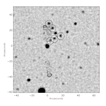
Figure 7: The $I$-band image of MRC B0058–229 with the 4860 MHz VLA radio contours overlaid. The quasar is located at 0,0; North is up, East is left. Galaxies with $20<I<22$ and $2.6<V-I<2.8$ are circled. These appear closer to the shorter, northern radio lobe.

4.3.3 MRC B0209–237, $z=0.680$

The value of $B_{gq}$ ($1377\pm 507$) and the $>10\sigma$ overdensity in Figure 4 suggest the presence of a rich cluster of galaxies. There are 13 objects with $20<I<23$ and $2.0<V-I<2.5$ in the 0.5 Mpc circle centred on the quasar compared with 32 in the rest of the field. This represents a density of $3.7$ arcmin^-2 near the AGN as opposed to $0.6$ arcmin^-2 in the field, a six-fold overdensity. The quasar is not found at the centre of the galaxy distribution, the majority of cluster galaxies being to the south of the quasar. The radio contours show that the southern radio lobe is shorter than the northern one, indicative of a denser ICM to the south (Figure 8).

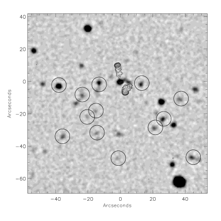
Figure 8: The $I$-band image of MRC B0209–237 overlaid with the 4860 MHz VLA radio contours. The quasar is at 0,0; North is up, East is left. Galaxies with $20<I<23$ and $2.0<V-I<2.5$ are circled.

4.3.4 MRC B0346–279, $z=0.989$

The quasar has large values of $B_{gq}$ and $N_{0.5}$ ($1957\pm 1207$ and $16.0\pm 3.3$) and there are a large number of faint objects ($23.0<R<24.0$) to its west. However, no overdensity is seen in Figure 4. On closer inspection, the colours of the objects which contribute to the large values of $B_{gq}$ and $N_{0.5}$ are too blue to be ellipticals at $z=0.989$. Figure 9 shows the surface density of galaxies in different colour slices. Redshift 1 ellipticals are expected to have $1.5<R-z<2.0$. The overdensity in the field of MRC B0346–279 is caused by objects with $0.0<R-z<1.0$, about 1 magnitude bluer. Therefore, this is more likely a lower-$z$ overdensity.

Only 10 objects are detected in NIR of which 3 have $R-K^{\prime}>5$. The completeness limit of the NIR data is $K^{\prime}=19.0$, giving most objects an upper limit of $R-K^{\prime}\sim 4-5$. For a $z=0.989$ cluster of galaxies we should expect to see objects with $18<K^{\prime}<19$ and $R-K^{\prime}>5$. The median colours for objects with $18<K^{\prime}<19$ in this field are $R-K^{\prime}\sim 3$ and $J-K^{\prime}\sim 1$ (Figure 10). These colours indicate relatively low-redshift galaxies (Figure 1).

If the objects around MRC B0346–279 were to comprise a cluster it would be highly unusual as the system has no discernible red galaxy population. This would be unique, even among the few high-redshift clusters known to date. Deep multi-object spectroscopy of this field will be required to resolve these issues. At present, we classify MRC B0346–279 as residing in an environment indistinguishable from the field with a concentration of objects in the foreground.

Figure 9: The density enhancements of objects of different colours in the field of MRC B0346–279. The contours represent units of 2, 3 and 5 $\times$ the Poisson noise of the background. The position of the quasar is marked by the asterisk. Passively-evolving ellipticals at $z=0.989$ are expected to appear in the $1.5<R-z<2.0$ panel.

4.3.5 MRC B0450–221, $z=0.898$

A cluster of galaxies has been detected about this quasar. There is an overdensity of galaxies with the optical – NIR colours of 0.898 elliptical galaxies and an enhancement of emission-line galaxies (ELGs). Preliminary spectroscopy confirms that the ELGs are at the redshift of the quasar [Baker et al. 2001].

The ambiguous value of $B_{gq}$ ($335\pm 300$) for MRC B0450–221 supports the use of the multicolour detection algorithm. Despite the relative richness of the cluster, $B_{gq}$ is hardly significant as a pure overdensity and would not have alerted investigators to the presence of clustering. The richness of the field further than 0.5 Mpc from the quasar contributes to the dilution of $B_{gq}$. As well as this, the high redshift of the source allows only a fraction of its galaxy population to be visible above the completeness limit.

4.3.6 MRC B0941–200, $z=0.715$

Optical and NIR observations of this field have been reported in Bremer et al. (2002). They discovered evidence for an excess of galaxies to the north-east with magnitudes $20<I<23$ and colours $1.05<R-I<1.25$. This extension of red objects is also evident in Figure 4 (which was compiled from independent data from that used by Bremer et al.). The quasar has a dramatically shorter southern lobe which is coincident with a spectrally confirmed compact group of galaxies at the quasar’s redshift.

4.3.7 MRC B1006–299, $z=1.064$

The value of $B_{gq}$ for this field is large ($2092\pm 1304$) and there is a $4\sigma$ peak in the density of objects with $1.5<R-z<2.0$ within 0.5 Mpc of the RLQ (Figure 4).

The NIR evidence points to this overdensity being a lower redshift system. Figure 11 shows a clear excess of objects with $K^{\prime}\sim 18$ and $R-K^{\prime}\sim 4$, $J-K\sim 1.5$ compared with MRC B0346–279 (Figure 10). However, the $R-K^{\prime}$ vs. $K^{\prime}$ red sequence expected for clusters at $z\sim 1$ is $\sim 1$ mag redder than these colours (shown as the solid line in Figure 11). Within the NIR field of view there are 13 objects with $4.3<R-K^{\prime}<4.9$, located mostly to the NE of the quasar in the region of the $4\sigma$ optical overdensity (Figure 12). The magnitudes of these principal members are $22.0<R<22.5$. These colours and magnitudes are indicative of bright cluster members at $z\sim 0.8$ [Snellen et al. 1996, Aragón-Salamanca et al. 1998].

Figure 10: The colour-magnitude diagram of objects in the $2^{\prime}\!\!.6$ $\times$ $2^{\prime}\!\!.6$ field around MRC B0346–279. The thick line represents colour-magnitude relation for a cluster at $z=0.989$, based on the observed colours of Coma early-types (Stanford et al. 1998). No red sequence is seen.

Figure 11: The colour-magnitude diagram of objects in the $2^{\prime}\!\!.6$ $\times$ $2^{\prime}\!\!.6$ field around MRC B1006–299. The thick line represents the no-evolution colour-magnitude relation for early-type galaxies at $z=1.064$, based on the observed colours of Coma early-types (Stanford et al. 1998).

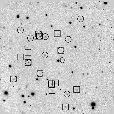
Figure 12: Objects in the field of MRC B1006–299 with $17<K^{\prime}<19$ and $4.3<R-K^{\prime}<4.9$ (circles), $1.7<J-K^{\prime}<2.3$ (squares). The image is the $2^{\prime}\!\!.6$ $\times$ $2^{\prime}\!\!.6$ $J$-band image and the quasar is labelled Q. North is up, East is left.

There is clearly a system of associated galaxies in this field as evinced by the proximity of objects both in space and colour. The projected density of objects with $K>19$ and $3.0<I-K<3.8$ is 6 times that found in the $47^{\prime}\!\!.2$ Herschel deep field [McCracken et al. 2000].

The magnitude and optical-NIR colour of the clustering objects imply that they are not at the same redshift as the quasar but at $z\sim 0.8$. Spectroscopy on 8m-class telescopes is required to fully characterise the nature of this field. For the present, it is classified as a quasar in a field environment with a cluster of galaxies in the foreground.

4.3.8 MRC B1202–262, $z=0.786$

The values of $B_{gq}$ and $N_{0.5}$ ($470\pm 232$ and $4.2\pm 5.1$) are inconclusive. Figure 4 shows $3\sigma$ overdensities of red galaxies NE and SW of the quasar. Unfortunately, without further optical or NIR images of this field we are unable to determine whether these overdensities are real systems of galaxies or chance superpositions. Classification of the environment of MRC B1202–262 will have to wait for deeper imaging or spectroscopy.

4.3.9 MRC B1208–277, $z=0.828$

Figure 4 shows a $3\sigma$ overdensity of objects with $V-I>2.0$ centred on the quasar.

There are $>4$ times as many galaxies with $K^{\prime}<19$ and $3.0<I-K^{\prime}<3.8$ within the NIR field of view than are expected from observations of the Herschel deep field [McCracken et al. 2000]. Figure 13 shows that these objects make up a red-sequence consistent with a $z=0.828$ cluster of galaxies.

Figure 13: The colour-magnitude diagram of objects in the $2^{\prime}\!\!.6$ $\times$ $2^{\prime}\!\!.6$ field around MRC B1208–277. The thick line represents colour-magnitude relation for the cluster MS 1054.5-0321 at $z=0.828$, based on the observed colours of Coma early-types (Stanford et al. 1998).

Figure 14 and Figure 15 show that candidate cluster members display a tendency to align themselves NW – SE. This is the same direction as the radio lobes (shown in Figure 15). Five of the objects so distributed are close doubles or have a disturbed morphology.

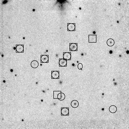
Figure 14: Objects in the field of MRC B1208–277 with $17<K^{\prime}<19$ and $3.0<I-K^{\prime}<3.8$ (circles), $1.7<J-K^{\prime}<2.1$ (squares). The image is the $2^{\prime}\!\!.6$ $\times$ $2^{\prime}\!\!.6$ $J$-band image and the quasar is labelled Q. North is up, East is left.

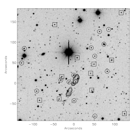
Figure 15: The $I$-band image of the field of MRC B1208–277 overlaid with the 4860 MHz VLA radio contours. Indicated are objects with $19<I<21$ and $2.0<V-I<2.5$ (circles) and $2.5<V-I<3.0$ (squares). North is up, East is left and the quasar is at 0,0. The large-scale structure of galaxies appears aligned with the radio lobes in a SE-NW direction.

The $V$-band magnitudes of candidate cluster members display a greater variation than expected of a cluster of galaxies at this redshift. Observations of MS 1054–03 indicate that core ellipticals have $V-I\sim 2.9$ [van Dokkum & Franx 2001] at $z=0.828$. Candidate core cluster galaxies around MRC B1208–277 have median $V-I\sim 2.4$, ie: half a magnitude bluer than ellipticals in MS 1054–03. Small amounts of on-going star formation can affect the $V$-band magnitude at these redshifts and could explain this discrepancy.

4.3.10 MRC B1224–262, $z=0.768$

A $5\sigma$ overdensity is seen in Figure 4 with $2.5<V-I<3.0$, the colour of passively-evolving ellipticals at $z=0.768$.

There are 6 objects within 0.5 Mpc with $20.5<I<22.5$ and $4.5<R-K^{\prime}<5.2$ and $1.38<R-I<1.58$ (Figure 16). The tightness of these colours, as well as the colours themselves point to the fact that these galaxies are located in the same system at the redshift of the quasar.

Figure 16: Co-added $V,R,I$ image of the central $2^{\prime}\times 2^{\prime}$ around MRC 1224–262 (labelled Q). Objects with $20.5<I<22.5$ and $4.5<R-K^{\prime}<5.2$ are indicated. The area shown here is that covered by the NIR field of view, North is up, East is left.

This is a sparse field, as evinced by the total number of objects in the colour-magnitude diagram. Nevertheless, it is possible to identify a red sequence in $I-K^{\prime}$ and $J-K^{\prime}$ in Figure 17.

Figure 17: The colour-magnitude diagram of objects in the $2^{\prime}\!\!.6$ $\times$ $2^{\prime}\!\!.6$ field around MRC B1224–262. The thick line represents no-evolution colour-magnitude relation for early-type galaxies at $z=0.768$, based on the observed colours of Coma early-types (Stanford et al. 1998).

The number of objects within the central square arcminute around the AGN with $2.6<I-K<3.8$ and $K<19$ is seven times that expected from analysis of the Herschel deep field [McCracken et al. 2000]. It must also be borne in mind that our data is incomplete above $K^{\prime}=18.5$ and so fainter objects in the field are missed; thus the true overdensity is likely to be greater than this.

MRC B1224–262 resides in an overdensity of galaxies consistent with being at $z=0.768$. We have identified candidate core cluster members, (Figure 16, and a possible red sequence, Figure 17). Although there are relatively few of these, this system does not satisfy the modified Hickson isolation requirement and thus is not classified as a compact group. The overdensity around MRC B1224–262 may be a loose grouping or a poor cluster of galaxies.

4.3.11 MRC B1301–251, $z=0.952$

No estimate of $B_{gq}$ is possible because of the insufficient depth of the $I$-band image. However, a $4\sigma$ overdensity in Figure 4 and the spatial distribution of galaxies with the colours of passive ellipticals at $z=0.952$ in Figure 18 indicate clustering of galaxies centred on the quasar.

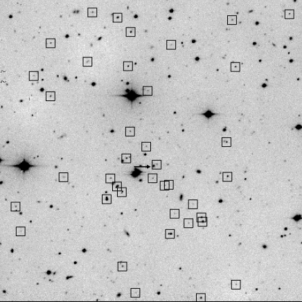
Figure 18: Objects in the field of MRC B1301–251 with $19<z<23$ and $2.8<V-z<3.4$. The quasar is marked with the horizontal arrow. The field of view is $4^{\prime}\!\!.9$ $\times$ $4^{\prime}\!\!.9$, North is up, East is left.

The $H$-band image only covers an area of $1$ square arcminute, as shown in Figure 19. Nevertheless, there are 7 objects with $19<H<21$ and $1.8<I-H<3.0$. This density is three times that of objects with similar colours in the Herschel deep field (assuming $H-K^{\prime}=1$ for ellipticals at $z=0.952$). The number and density of these objects around MRC B1301–251 point to the presence of a cluster of galaxies.

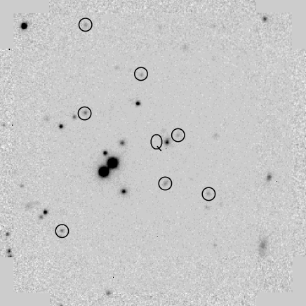
Figure 19: The $H$-band image of the central arcminute about MRC B1301–251, North is up, East is left. Indicated are those objects with $1.8<I-H<3.0$ and $H<21$. The quasar is marked with the Q.

4.3.12 MRC B1303–250, $z=0.738$

Figure 4 shows a $3\sigma$ peak in the density contrast to the east of the RLQ. VLA observations show a bent radio source [Kapahi et al. 1998], possibly indicating interaction with an ICM. However, as is the case with MRC B1202–262, this is the extent of the information on this source. MRC B1303–250 may reside on the edge of a cluster of galaxies, however more detailed imaging/spectroscopy will be required before this can be confirmed.

4.3.13 MRC B1355–236, $z=0.832$

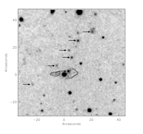
Figure 20: The central $\sim 1^{\prime}$ of the $I$-band image of MRC B1355–236 overlaid with the 4860 MHz VLA radio contours. Objects with $20<I<23$ and $1.2<R-I<1.5$ are indicated. North is up, East is left, the quasar is at 0,0.

There is a linear clustering of objects to the NW of the quasar. Figure 20 shows seven objects with $20<I<23$ and $1.2<R-I<1.5$, consistent with being $z=0.832$ ellipticals. The most north-western member of the system has a very diffuse morphology and may be a merger. There is marginal ($3\sigma$) clustering of objects with these magnitudes and colours to the East of the quasar (Figure 4). For this reason the system does not conform to Hickson’s isolation criterion and so could be a cluster core or a compact group on the edge of a poor cluster rather than an isolated compact group. Wide-field NIR imaging or MOS is required to classify the environment of MRC B1355–236 more accurately.

4.4 Summary

The fields of all 21 quasars in this sample were examined for signs of clustering. Objects with $>3\sigma$ overdensities in the density maps were set aside as cluster candidates and examined further. Those fields with $>5\sigma$ overdensities, or $>3\sigma$ with an enhancement of NIR number counts over field estimates were classified as clusters of galaxies. The fields were then examined to see if they complied with the modified Hickson requirements to qualify as a compact group.

The analysis reveals clustering of galaxies in the fields of 8 quasars. In two cases, MRC B0058–229 and MRC B0941–200, the clustering is consistent with being a compact group. Poor or missing data meant that no determination can be made as to the nature of 3 fields (labelled ‘?’ in Table LABEL:tab:bgq). In two cases (MRC B0346–279 and MRC B1006–299) high values of $B_{gq}$ and $N_{0.5}$ are likely to be caused by intervening systems of objects. All other (8) objects have environments consistent with other galaxies in the field. The classifications are listed in Table LABEL:tab:bgq.

The mean $B_{gq}$ values of the clustered systems (C/G) are systematically richer than those of the fields (F), $436\pm 178$ as opposed to $159\pm 150$. However, there is considerable overlap in the statistics when individual fields are examined. This suggests that $B_{gq}$ is only useful as an ensemble statistic and is not necessarily an accurate predictor of a single high-redshift quasar’s environment. For a further discussion of this point see §5.4.

5 Discussion

5.1 Clustering in the fields of RLQs

We find strong evidence for clustering of galaxies about quasars in the fields of 8 of the 21 RLQs (C or G in Table LABEL:tab:bgq). The nature of the clustering varies from compact groups to rich clusters. Marginal evidence for clustering is seen in 3 other fields (labelled as ‘?’ in Table LABEL:tab:bgq). In two further cases, MRC B0346–279 and MRC B1006–299, suspected intervening systems of galaxies are found. The rest of the quasars have environments consistent with field galaxies.

The clusters of galaxies found in this work are selected based on their old elliptical population. This means that in the systems at $0.6<z<1.1$ detailed in §4.3, the passively-evolving elliptical core galaxies are already a significant constituent. Other studies of (richer) clusters of galaxies at these redshifts (eg: Stanford et al. 1998; van Dokkum & Franx 2001) find a similar state of affairs. Results such as these have been used to argue that the formation epoch of the majority of stars in early-type galaxies is $z\sim 2-3$ (van Dokkum & Franx 2001; see also §5.2).

Targetting quasars is a very efficient way of finding structure at high redshift. We find compact groups or clusters of galaxies in at least $\sim 40\%$ and possibly $>50\%$ of our RLQ fields, a return of $\sim 40$ clustered systems per square degree imaged (nb: not $\sim 40$ clusters per square degree of sky). This compares favourably with current high-redshift cluster surveys, eg: $\sim 1-2$ clusters at $z\lesssim 1.2$ per square degree for the Red-Sequence Cluster Survey [Gladders & Yee 2000] or the predicted $\sim 10$ clusters per square degree at $0.6<z<1.1$ for the XMM-LSS [Romer et al. 2001, Refregier, Valtchanov & Pierre 2002].

We have shown that detecting clustered systems above a redshift of 0.6 with 4m data and single-filter techniques is difficult. With the addition of colour information and NIR filters it is possible to extend the searches above $z=1$. These limits are comparable in terms of depth with the most recent wide-field optical and X-ray surveys. In order to study clustered systems at redshifts of 1 to 2 or greater, 8m data will be required. Observations in this redshift range are desirable because it represents the peak in the star formation activity of the universe (Madau, Pozzetti & Dickinson 1998), the period of maximum AGN activity [Hartwick & Schade 1990, Peterson 1997] and possibly the epoch of major cluster assembly. It is likely that the interplay between these distinct phenomena can be disentangled using observations of clustered fields at $z\sim 2$. However, most 8m telescopes have cameras with a field of view of $\sim 5^{\prime}$. It would therefore take a prohibitively long time to complete a survey with these facilities. The XMM-LSS will detect systems at $z=1-2$ but numbers will be weighted significantly toward $z=1$, with few at $z\sim 2$. Until coordinated X-ray and SZ searches come on line, the only way to detect systems of galaxies efficiently at redshift $\sim 2$ is to use targetted searches.

Imaging the fields of quasars also represents a means of compiling complimentary catalogues to those of other cluster surveys. The fields of RLQs are typically poorer than the systems identified by optical or X-ray means, and they are likely to be less massive than the clusters SZ observations will discover. However, in common with systems detected by these means, our clusters display no evidence for evolution to $z\gtrsim 0.9$ (Lubin 1996; Ebeling et al. 1998, but see Gioia et al. 2001) . We also detect the presence of a red sequence in our clusters. This indicates that like richer clusters, their passively-evolving ellipticals formed at $z\gtrsim 2$ [Stanford et al. 1998, Holden et al. 2001, van Dokkum & Franx 2001].

5.2 Colours of core cluster galaxies

Figure 21: Average SEDs for red objects in the fields of clusters. The data points are compiled from the objects with the colours of passively-evolving ellipticals at the quasar redshift (see Figure 4 for the precise selection criteria) calibrated to AB magnitudes. Model elliptical galaxy spectra from Fioc & Rocca-Volmerange (1997) are shown with a $\lambda^{-1.3}$ reddening dependence added. The solid line represents a 6 Gyr, and the dashed line a 2 Gyr old galaxy.

Assuming that core cluster galaxies have certain colours carries a central disadvantage, namely that minimal analysis can be undertaken to investigate the properties of these colours. However, some analyses can be made. One important test involves the spectral energy distributions of galaxies and is featured in Figure 21.

There are four cluster fields for which at least two optical and at least two NIR images exist. It is these latter NIR filters that are essential to provide enough of a baseline over which to test different SEDs. Data points in each filter were assembled by considering only objects with the colours of passively-evolving ellipticals at the quasar redshift, ie: those galaxies used to construct the panels in Figure 4. These were then converted to AB magnitudes using the prescriptions of Fukugita et al. (1995).

The spectra were assembled from the models of Fioc & Rocca-Volmerange (1997), redshifted to the appropriate epoch and scaled to fit the points as well as possible. Six Gyr and two Gyr elliptical models were considered, both with solar metallicity and an exponentially decreasing star formation rate. There are no good fits to the resulting spectrum unless some host galaxy reddening is applied. Bremer et al. (2002) found that spectroscopic observations of the galaxies in the MRC B0941–200 group can be made to agree well with a 3 Gyr model if a $\lambda^{-1.3}$ reddening dependence is introduced. This is therefore applied to the models, normalising to $A_{V}=0.4$ for consistency with observations.

The resulting SED comparisons are shown in Figure 21. The data is well fit by elliptical galaxies with stellar masses of $\sim 10^{11}$M_⊙, ages of $2-6$ Gyr and on-going star formation rates of $0.5-2$ M_⊙yr^-1. For the fields of MRC B0450–221 and MRC B0941–200 the data points favour the older model while in the other two fields no preference is found.

These data indicate that at $0.7<z<0.9$, the elliptical population is at least $2$ Gyr old and potentially $6$ Gyr old. This suggests that the passively-evolving galaxies in the cores of the clusters form at redshifts of $2-3$. If passively-evolving ellipticals form at $z\gtrsim 2$ and are in place at $z\sim 1$ the indications are that a cluster will not have had time to virialise. The time between these redshifts is $\sim 3-4$ Gyr whereas virialisation timescales are typically many Gyr for cluster mass scales. Even at $z=0$, the outer parts of many clusters are not dynamically relaxed. Certainly, the distributions of the ellipticals about the RLQs and the positions of the quasars in their putative clusters (see §5.3) suggest that these systems are not virialised.

5.3 The distribution of galaxies around RLQs

In nearly all cases in which clustering is evident, there is a $\sim 10^{\prime\prime}-20^{\prime\prime}$ distance between the RLQ and the centroid of the red galaxy distribution. This is illustrated graphically in Figure 22. The figure shows the projected distance between the peak value of the clustering statistic (as calculated in §4) and the RLQs. These distances are only determined for points within 500kpc of each quasar. If there is no overall correlation between the quasar position and cluster peak, the peak-to-RLQ distance should increase steadily to a maximum value of $\sim 60^{\prime\prime}-80^{\prime\prime}$, a reflection of the greater area sampled at increased radii. This is exactly what happens to the quasars in field environments. However, RLQs marked ‘C’ or ‘G’ in Table LABEL:tab:bgq show a marked tendency to exist $10^{\prime\prime}-20^{\prime\prime}$ away from the cluster peak. Of the two quasars which do not obey this relationship, there is evidence that both MRC B0941–200 and MRC B1355–281 exist in a compact group at the edge of a larger-scale structure (§4.3).

The panels in Figure 4 and Figure 23 also indicate that quasars in the sample are not necessarily found at the centres of galaxy clusters. However, without X-ray data, it is not possible to tell whether an AGN truly resides at the edge of a cluster or whether the galaxy distribution fails to follow the gravitational potential faithfully. The optical study of Cygnus A and its surrounding cluster of galaxies by Owen et al. (1997) shows that the powerful radio source is offset by $\sim 10^{\prime\prime}$ from the galaxy distribution. However, in this case the radio galaxy is found at the bottom of the potential well, as traced by the X-ray emitting gas [Smith et al. 2002].

Clustering of galaxies also extends further than $100^{\prime\prime}$ ($\sim 1$ Mpc) from the RLQs, eg: MRC B0030–220, MRC B0058–229, MRC B0941–200, MRC B1208–277 in Figure 4. Similar results have been observed by Sánchez and González-Serrano (1999; 2002) for (non colour-selected) galaxies in the fields of 7 RLQs at $1.0<z<1.6$.

Figure 22: Thick line: Histogram showing the projected distance between the peak value of the clustering statistic (as calculated in §4) and the RLQs denoted ‘C’ or ’G’. Dotted line: The same but for those quasars categorised as ‘F’ (Table LABEL:tab:bgq). In both cases the distance is calculated only within 500kpc of each quasar.

.

Figure 23: The spatial cross-correlation amplitude at all points in the fields of four quasars which reside in clusters. The quasars are marked by an asterisk, North is up, East is left.

In general, the distribution of passive ellipticals in the clustered systems is irregular. None of the agglomerations display obvious spherical symmetry. This may be a product of shallow sampling, or may reflect the genuine topology of the systems. The fact that the quasars themselves (and by implication their massive elliptical hosts) are not centred on the elliptical distribution may indicate the second of these options. Other observations have suggested that rich high-redshift clusters can display an irregular X-ray morphology [Donahue et al. 1998], indicating further that the poorer clustered systems in this work are likely to be unvirialised, or are made up of several smaller-scale virialised components.

The fact that RLQs are not found at the centre of galaxy clusters and the projected extension of these distributions can be used to explain the results of Hall & Green (1998). Hall & Green found that overdensities of $K\gtrsim 19$ around $1<z<2$ RLQs occurred on two spatial scales. The first was a significant enhancement at $<40^{\prime\prime}$ from the quasars compared with the rest of the field. The second was a higher density over the $\sim 100^{\prime\prime}$ field of view compared with literature values.

Asymmetric clustering of galaxies about RLQs can, when the results are combined, reproduce this sort of distribution. Figure 24 shows the result of simulated clusters placed in the fields of quasars. In 50 out of 100 cases, ‘clusters’ of $\sim 20$ objects were placed with their centre anywhere within $50^{\prime\prime}$ of a ‘quasar’. This quasar was itself the centre of a ‘field’ of about 20 objects randomly placed in a $300^{\prime\prime}$ square area. The numbers were chosen to reproduce roughly the $K$ band number counts which were the basis of Hall & Green’s selection. The resulting distributions of objects were stacked and the density of objects was calculated in the same manner as Figure 4. Figure 24 shows a $>4\sigma$ overdensity within $40^{\prime\prime}$ of the quasar which resembles Hall & Green’s $4.5\sigma$ overdensity within $40^{\prime\prime}$ rather closely. An overdensity of objects over the whole field relative to the background counts is also expected. The edge of particular cluster can reach to $\sim 100^{\prime\prime}$ from the quasar thereby producing an overdensity, albeit of low significance, relative to the field.

Figure 24: Contour plot showing the density of objects in multiple, simulated clusters. Each cluster is created by placing objects randomly in a $50^{\prime\prime}$ radius and offset by up to $\sim 50^{\prime\prime}$ from the quasar. The results are stacked and the average density is found as with Figure 4 (see text). The contours are in units of $\sigma$.

The simulations suggest that Hall & Green’s results can be reproduced if, as found with the RLQs in this work, about half the fields have galaxy excesses asymmetrically distributed within $\sim 50^{\prime\prime}$ of the quasar.

5.4 Single-filter clustering statistics

We have calculated $B_{gq}$ and $N_{0.5}$ for our sample of objects and find them to be consistent with previous, lower redshift studies. We find no evidence for evolution in clustering, measured thus, with redshift. The assertion that there is large variance in the clustering of galaxies around quasars is also supported by these results.

Five of the eight groups and clusters of galaxies found using multicolour means (labelled ‘C’ or ‘G’ in Table LABEL:tab:bgq) have insignificant or incalculable values of $B_{gq}$. This partly reflects the fact that these systems are poorer. However, it is also due to the lessening of the efficiency of the statistic with epoch. There are various reasons why this occurs. At the highest redshifts ($z>0.9$) the depth of the data only allows imaging of the brightest cluster members. These several galaxies then do not constitute a significant population and may be overwhelmed by foreground galaxies at the same magnitude levels.

In attempting to compare clusters over a range of $z$, investigators assume that the cluster morphology is independent of redshift. In particular, when interpreting $B_{gq}$ and $N_{0.5}$ as a measure of cluster richness, it is assumed that the quasar resides at the centre of the galaxy distribution. It is known, however, from studies of the most powerful high-redshift X-ray clusters that these systems may be less regular than their low-redshift counterparts and exhibit considerable sub-structure (eg: MS 1054-03; Donahue et al. 1998; van Dokkum & Franx 2001). Section 5.3 also showed that the quasar does not reside in the centre of a galactic overdensity. This means that $B_{gq}$ or $N_{0.5}$ can always be made greater by placing the centre of the 0.5 Mpc circle used to calculate $A_{gq}$ somewhere other than on the quasar. Figure 23 illustrates this graphically. The spatial cross-correlation function is calculated for four clusters in the sample. $B_{gq}$ is calculated at all points within a 200^′′ square centred on the quasar assuming the clustering is at the redshift of the quasar. In all cases in Figure 23 it is evident that the value of the spatial cross-correlation amplitude is not maximal at the quasar position but is always offset by some 20^′′ to 50^′′ (cf: also Figure 22). This will lead to a systematic underestimate in the richness of a system. At lower redshift it has been assumed that the quasar is found in the central cluster galaxy and thus that an Abell richness can be derived from $B_{gq}$. This work shows that this is not the case and at $z>0.6$ it seems likely that an Abell class cannot be reliably be assigned to a particular value of $B_{gq}$.

Intervening systems of galaxies also distort the values of $B_{gq}$ and $N_{0.5}$. $B_{gq}$ for 2 of the 21 quasars in the sample, MRC B0346–279 and MRC B1006–299, would lead them to be classified as rich clusters at redshifts 0.989 and 1.064 respectively. Section 4.3 has shown that these overdensities are not consistent with clusters of galaxies at these redshifts. This suggests that $\sim 10\%$ of values of $B_{gq}$ for quasars at $z\sim 1$ are overestimated due to the presence of foreground systems.

Selecting clusters of galaxies by the red colours of their passive elliptical population circumvents some of the problems mentioned above. The colours of these galaxies are rare (or at least are made so by the appropriate choice of filters), so dilution by faint foreground galaxies becomes much less of an issue. The multicolour method also has the power to reject intervening systems.

5.5 Radio Properties

A full discussion of the radio properties of the sample will be presented in Barr et al. (2003, in preparation). For the time being, we note two clustering trends involving the radio morphology of our sample. Firstly that clustered environments are preferably associated with sources whose sizes are $<200$kpc, while larger radio sources are found in unclustered environments. Secondly, asymmetric radio sources are almost always associated with clustered environments, though not necessarily rich clusters.

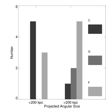
Figure 25: Bar plot showing the dichotomy in projected angular size for sources in field (F), compact groups (G) and cluster (C) environments.

Figure 25 shows clustering about our RLQs based on the projected angular size of the source. Of the 21 sources, those whose environments could not be classified are excluded. MRC B0346–279 and MRC B1055–242 are also removed because they are unresolved flat-spectrum objects and therefore yield information only on their cores, the lobes being either too small or too diffuse to be observed. MRC M1355–236 is classified as a cluster in this analysis because it does not satisfy the modified Hickson requirements to qualify as a compact group. All other objects are classed according to column 6 of Table LABEL:tab:bgq.

Figure 25 suggests that clusters of galaxies are often associated with smaller steep-spectrum radio sources. The Binomial probability of obtaining this distribution at random from the fields detailed in Figure 25 is $10\%$.

The source size/clustering relation cannot be one-to-one. We would expect to see small sources in poorer environments for two reasons. Firstly, the age of the source must be a factor. A young radio source cannot tell us anything about the environment it has yet to expand into. Secondly, projection effects may serve to foreshorten large-scale radio structures of sources in poor environments, weakening the correlation between angular size and clustering. This second effect will not be large as we exclude core dominated objects so removing the most extremely foreshortened objects from the sample.

Table 4: Characteristics of radio sources with short lobe to long lobe ratios of$\leq 0.67$ in our sample. The shorter lobe side is indicated by the letter in the second column.

MRC Object	Approx lobe	Cluster	F/G/C
	size ratio	side
B0058–229	0.67N	N	G
B0209–237	0.59S	S	C
B0450–221	0.67NW	NE	C
B0941–200	0.30S	S	G
B1208–277	0.55N	S	C
B1301–251	0.59W	NE	C

There is a correlation between clustering about our radio sources and their asymmetry. The short-to-long lobe length ratios of all sources were determined by calculating the distance from the optical identifications to the peak in the radio in each lobe. We find that all sources with lobe length ratios $\leq 0.67$ are associated with clustering (Table 4 ). Of sources that display less asymmetry, only 5 of 15 show signs of clustering. This suggests that a source’s asymmetry is a strong function of the other galaxies in its environment.

Of our asymmetric sources, the shortest lobe points toward the main body of clustering galaxies in only half of the cases. If the lobe length asymmetry is caused by density gradients in an ICM, this would indicate that the galaxy and gas distributions are not necessarily closely related. However, we note that of the six sources in Table 4, the short lobe and cluster coincide for the three lower redshift sources. Deeper images of sources above $z=0.8$ may reveal a different galaxy distribution. Foreshortening of bent sources can also complicate matters. Nevertheless, the high correspondence of asymmetry and clustering indicates that cluster ICM affects radio structure considerably.

Cluster searches based on radio-loud AGN selection are currently highly-efficient means of finding high-redshift systems of galaxies. Evidence from analysis of radio morphology suggests that selecting sources based on radio size and asymmetry can improve the efficiency of these searches still further.

6 Conclusions

We have described the environments of a representative sample of RLQs in terms of the colours of galaxies which surround them. Of the 21 sources, we have identified clustering of galaxies around 8 of them. Three further sources show signs of clustering but require more accurate observations to confirm. Two other sources display strong evidence for a lower-redshift galaxy systems in their fields. The other 8 quasars in the sample reside in environments indistinguishable from the field.

As found at lower redshifts, powerful low-frequency-selected radio-loud quasars at redshift $0.6<z<1.1$ exist in a wide variety of environments, from field through compact groups to rich clusters. There is no evidence for evolution in clustering richness as we progress to higher redshifts.

The colours of galaxies in the RLQ-selected clusters are suggestive of passively-evolving ellipticals with no more than a small amount of on-going star formation. The quasar is not always directly centred on any overdensity, nor is clustering confined to within 0.5 Mpc of the active galaxy. This contrasts with clusters at lower redshift where quasar host galaxies, massive ellipticals, appear to reside at the centre of a relaxed galaxy distribution. It also conflicts with the assertion presented above that the environments of these sources do not vary with redshift.

The positions of the quasars and the distribution of the galaxies suggest that these clusters are not virialised. This indicates that massive elliptical galaxy formation is favoured in overdense regions or virialised subclumps and that the old, red galaxies are in place before the cluster becomes relaxed.

We have shown that using colour information to describe environment is a more precise way than quantifying the clustering based on observations made in a single filter. Indeed, it avoids several of the pitfalls associated with these clustering statistics; namely the increased cosmic variance at these faint magnitude levels, the offset of the RLQ from the centre of the galaxy distribution and signals caused by foreground objects. We predict that where $B_{gq}$ has been used to quantify clustering above $z=0.6$, it will systematically underestimate the clustering richness of true clusters. In about $10\%$ of cases at $z\sim 1$, $B_{gq}$ may be influenced by the presence of foreground systems.

The smallest extended sources show a strong association with clusters of galaxies. Asymmetric sources are also more likely to be classified as being in clustered environments (though not necessarily in the richer systems). Discrimination on size and asymmetry results in an extremely efficient way of selecting high-redshift groups and clusters. Despite the obvious effectiveness of colour selection in detecting these systems, follow-up 8m imaging and spectroscopy is still required to determine the parameters of the systems.

Appendix A Single-filter clustering statistics

A.1 Galaxy-quasar cross-correlation amplitude, $B_{gq}$

The amplitude of the spatial cross-correlation function has been used as a measure of galaxy excess by many investigators, initially Seldner & Peebles (1978) and Longair & Seldner (1979). Its application to probe the environments of AGN at various redshift is also well established [Yee & Green 1987, Ellingson et al. 1991, Wold et al. 2000, McLure & Dunlop 2001]. A detailed derivation can be found in Longair & Seldner (1979).

The spatial cross-correlation function, $\xi(r)$ measures the excess probability of finding a companion galaxy at a distance $r$ from the quasar. It is found to be well fit by the form,

$$\xi(r)=B_{gq}r^{-\gamma}\vspace{-0.5mm}$$

where $B_{gq}$ is the spatial cross-correlation amplitude and $\gamma$ is the power-law index. The value of $\gamma$ is usually assumed to be 1.77, the value for the low-redshift galaxy-galaxy correlation function as found by Groth & Peebles (1977). In order to determine $B_{gq}$ from our data, we must first find the angular cross-correlation amplitude, $A_{gq}$, from the angular counterpart to the spatial cross-correlation function,

$$\omega(\theta)=A_{gq}\theta^{1-\gamma}$$

For small $\theta$ the amplitude of the angular cross-correlation amplitude can be estimated from the data using the relation:

$$A_{gq}=\frac{N_{tot}-N_{b}}{N_{b}}\frac{{3-\gamma}}{2}\theta^{\gamma-1}$$

where $N_{tot}$ is the number of galaxies within a circle of radius $\theta$ centred on the quasar corresponding to 0.5 Mpc at the redshift of the quasar. $N_{b}$ is the expected number of background galaxies within $\theta$. The spatial cross-correlation amplitude is then obtained from $A_{gq}$ using:

$$B_{gq}=\frac{N_{g}A_{gq}}{\Phi(m_{lim},z)I_{\gamma}}d_{A}^{\gamma-3}$$ (1)

where $N_{g}$ is the average surface density of background galaxies and $d_{A}$ is the angular diameter distance to the quasar. $I_{\gamma}$ is an integration constant which has the value 3.78 for $\gamma$ = 1.77, and $\Phi$($m_{lim},z$) is the luminosity function integrated down to the completeness limit at the quasar redshift. This gives an estimate of the number of galaxies per unit volume to the limiting magnitude and introduces a degree of redshift independence into the statistic.

All of our images have a large enough field of view so that we can use the area further than 0.5 Mpc from the quasar to determine a “field density”. We then used this to predict a value of $N_{b}$, the number of objects expected within 0.5 Mpc of the quasar.

For the Schechter parameters, we follow the prescription given in W00 and use $\alpha=0.89$, $\phi_{V}^{*}=0.0065$, $\phi_{R}^{*}=0.0072$, $\phi_{I}^{*}=0.0052$ and $M_{V}^{*}=-21.04$, $M_{R}^{*}=-22.08$, $M_{I}^{*}=-22.65$. In order to probe as far down the luminosity function as possible, the deepest image in any particular field was used to calculate $B_{gq}$. This means where we had the choice, we first used the EFOSC $I$ band, then the EFOSC $R$ and then the CTIO $I$. In the case of the Taurus data which does not overlap with the EFOSC and CTIO data we had no choice, and the $I$ band was used to calculate $B_{gq}$. The errors were calculated using the conservative prescription of Yee & Lopez-Cruz (1999):

$$\frac{\Delta B_{gq}}{B_{gq}}=\frac{[(N_{tot}-N_{b})+1.3^{2}N_{b}]^{1/2}}{N_{tot}-N_{b}}$$

where the variables have the same meaning as before.

A.2 The Hill & Lilly Quantity, $N_{0.5}$

The quantity $N_{0.5}$ [Hill & Lilly 1991] provides a measure of spatial clustering which, unlike $B_{gq}$, does not depend on an estimate of the luminosity function at the redshift of the quasar. For a galaxy with apparent magnitude $m_{g}$, $N_{0.5}$ is defined as the number of excess galaxies within a projected 0.5 Mpc with magnitudes in the range $m_{g}$ to $m_{g}+3$. When looking at quasars, light from the AGN will dominate light from the host galaxy, making a direct measurement of $m_{g}$ impossible. $m_{g}$ is therefore estimated from the magnitude-redshift relation for radio galaxies of Eales (1985):

$$m_{g}(R)=21.05+5.3\mathrm{log}\,z$$ (2)

valid for $19.0<m_{g}<21.3$. Magnitudes for objects in the quasar fields which we imaged in colours other than $R$ (13 fields), were adjusted to $R$ using the colour relationships for redshifted E/S0 galaxies from Fukugita et al. (1995). The number density of expected objects was calculated from the region outside 0.5 Mpc as per the $B_{gq}$ formulation and the error from the $\sqrt{N}$ of this number. In several cases (indicated on Table LABEL:tab:bgq), the images are not deep enough for a complete catalogue of objects to $m_{g}+3$. In these cases $N_{0.5}$ is calculated to the completeness limit of the data as given Table 2. For a fuller description of $N_{0.5}$, again see W00.

Figure 26: Graph of $B_{gq}$ vs. $N_{0.5}$ for the 11 fields in our sample which are complete to $m_{g}+3$ for the $N_{0.5}$ calculation. The dashed line is the $N_{0.5}$ - $B_{gq}$ relation of W00, $B_{gq}=37.8N_{0.5}$. The horizontal lines indicate the normalisation between $B_{gq}$ and Abell classes as quoted in McLure & Dunlop (2001).

Figure 26 shows the relation between the spatial cross-correlation amplitude and the Hill and Lilly quantity for the fields that we have values of $N_{0.5}$ calculated using the full $m_{g}$ to $m_{g}+3$ magnitude range. We see a close relationship between the quantities as they both probe the clustering of the same faint objects in the fields of the quasars. As Figure 26 shows, there is agreement which is consistent with the relationship of $B_{gq}=37.8N_{0.5}$ quoted in W00.

References

- [Aragón-Salamanca et al. 1998] Aragón-Salamanca A., Baugh C.M., Kauffmann G. 1998, MNRAS, 297, 427
- [Balogh et al. 1997] Balogh M.L., Morris S.L., Yee H.K.C., Carlberg R.G., Ellingson E. 1997, ApJ, 488, L75
- [Baker et al. 1995] Baker J.C., Hunstead R.W., Brinkmann W. 1995, MNRAS, 277, 553
- [Baker 1997] Baker J.C. 1997, MNRAS, 286, 23
- [Baker et al. 1999] Baker J.C., Hunstead R.W., Kapahi V.K., Subrahmanya C.R. 1999, ApJS, 122, 29
- [Baker et al. 2001] Baker J.C., Hunstead R.W., Bremer M.N., Bland-Hawthorn J., Athreya R. M. Barr J.M. 2001, AJ, 121, 1821.
- [Baker et al. 2002] Baker J.C., Hunstead R.W., Athreya R.M., Barthel P.D., de Silva E., Lehnert M.D., Saunders R.D.E. 2002, ApJ, 568, 592
- [Barger et al. 1996] Barger A.J., Aragon-Salamanca A., Ellis R.S., Couch W.J., Smail I., Sharples R.M. 1996, MNRAS, 279, 1
- [Baum 1959] Baum W.A. 1959, PASP, 71, 106
- [Bertin & Arnouts 1996] Bertin E., Arnouts S. 1996, AASS, 117, 393
- [Bower, Lucey & Ellis 1992] Bower R.G., Lucey J.R., Ellis R.S. 1992, MNRAS, 254, 601
- [Bremer et al. 1992] Bremer M.N., Crawford C.S., Fabian A.C., Johnstone R.M. 1992, MNRAS, 254, 614
- [Bremer et al. 2002] Bremer M.N., Baker, J.C., Lehnert, M. 2002, MNRAS, 337, 470
- [Couch et al. 1991] Couch W.J., Ellis R.S., MacLaren I., Malin D.F. 1991, MNRAS, 249, 606
- [Donahue et al. 1998] Donahue M., Voit G.M., Gioia I., Lupino G., Hughes J.P., Stocke J.T. 1998, ApJ, 502, 550
- [Dressler 1980] Dressler A. 1980, ApJS, 42, 565
- [Drory et al. 2001] Drory N., Feulner G., Bender R., Botzler C.S., Hopp U., Maraston C., Mendes de Oliveira C., Snigula J. 2001, MNRAS, 325, 550
- [Eales 1985] Eales S.A. 1985, MNRAS, 217, 149
- [Ebeling et al. 1998] Ebeling H., Edge A.C., Bohringer H., Allen S.W., Crawford C.S., Fabian A.C., Voges W., Huchra J.P. 1998, MNRAS, 301, 881
- [Ellingson et al. 1991] Ellingson E., Yee H.K.C., Green R.F. 1991, ApJ, 371, 49
- [Fioc & Rocca-Volmerange 1997] Fioc M., Rocca-Volmerange B. 1997, AA, 326, 950
- [Fukugita et al. 1995] Fukugita M., Shimasaku K., Ichikawa T. 1995, PASP, 107, 945
- [Gioia & Luppino 1994] Gioia I.M., Luppino G.A. 1994, ApJS,94, 583
- [Gioia et al. 2001] Gioia I.M., Henry J.P., Mullis C.R., Voges W., Briel U.G., Böhringer H., Huchra J.P. 2001, ApJ, 553, L105
- [Gladders et al. 1998] Gladders M.D., Lopez-Cruz 0., Yee H.K.C., Kodama T. 1998, ApJ, 501, 571
- [Gladders & Yee 2000] Gladders M.D., Yee H.K.C. 2000, AJ, 120, 2148
- [Gross et al. 1998] Gross M.A.K., Somerville R.S., Primack J.R., Holtzman J., Klypin A. 1998, MNRAS, 310, 81
- [Groth & Peebles 1977] Groth E.J., Peebles P.J.E. 1977, ApJ, 217, 385
- [Hall & Green 1998] Hall P.B., Green R.F. 1998, ApJ, 507, 558
- [Hall, Green & Cohen 1998] Hall P.B., Green R.F., Cohen M. 1998, ApJS, 119, 1
- [Hartwick & Schade 1990] Hartwick F.D.A., Schade D. 1990, ARAA, 28, 437
- [Hickson 1982] Hickson P. 1982, ApJ, 255, 382
- [Hill & Lilly 1991] Hill G.J., Lilly S.J. 1991, ApJ, 367, 1
- [Holden et al. 2001] Holden B.P. Stanford S.A., van Dokkum P., Eisenhardt P., Dickinson M. 2001, American Astronomical Society Meeting, 199, 0
- [Hutchings 1995] Hutchings J.B. 1995, AJ, 109, 928
- [Ishwara-Chandra et al. 1998] Ishwara-Chandra C.H., Saikia D.J., Kapahi V.K., McCarthy P.J. 1998, MNRAS, 300, 269
- [Ishwara-Chandra et al. 2001] Ishwara-Chandra C.H., Saikia D.J., McCarthy P.J., van Breugel W.J.M. 2001, MNRAS, 323, 460
- [Jenkins et al. 1998] Jenkins A., Frenk C.S., Pearce F.R., Thomas P.A., Colberg J.M., White S.D.M., Couchman H.M.P., Peacock J.A., Efstathiou G., Nelson A.H. 1998, ApJ, 499, 20
- [Kapahi et al. 1998] Kapahi V.K., Athreya R.M., Subrahmanya C.R., Baker J.C., Hunstead R.W., McCarthy P.J., van Breugel W. 1998, ApJS, 118, 327
- [Kodama & Bower 2001] Kodama T., Bower R.G. 2001, MNRAS, 321, 18
- [Laing, Riley & Longair 1983] Laing R.A., Riley J.M., Longair M.S. 1983, MNRAS, 204, 151
- [Landolt 1992] Landolt A.U. 1992, AJ, 104, 340
- [Lidman & Peterson 1996] Lidman C.E., Peterson B.A. 1996, AJ, 112, 2454
- [Longair & Seldner 1979] Longair M.S., Seldner M. 1979, MNRAS, 189, 433
- [Lubin 1996] Lubin L.M. 1996, AJ, 112, 23
- [Madau, Pozzetti & Dickinson 1998] Madau P., Pozzetti L., Dickinson M. 1998, ApJ, 498, 106
- [Martini 2001] Martini P. 2001, AJ, 121, 598
- [McCarthy, Persson & West 1992] McCarthy P.J., Persson S.E., West S.C. 1992, ApJ, 386, 52
- [McLure & Dunlop 2001] McLure R.J., Dunlop J.S. 2001, MNRAS, 321, 515
- [McCracken et al. 2000] McCracken H.J., Metcalfe N., Shanks T., Campos A., Gardner J.P., Fong R. 2000, MNRAS, 311, 707
- [Olsen et al. 1999a] Olsen L.F., Scodeggio M., da Costa L., Benoist C., Bertin E., Deul E., Erben T., Guarnieri M.D., Hook R., Nonino M., Prandoni I., Slijkhuis R., Wicenec A., Wichmann R. 1999a, A&A, 345, 363
- [Olsen et al. 1999b] Olsen L.F., Scodeggio M., da Costa L., Slijkhuis R., Benoist C., Bertin E., Deul E., Erben T., Guarnieri M.D., Hook R., Nonino M., Prandoni I., Wicenec A., Zaggia S. 1999b, A&A, 345, 363
- [Owen et al. 1997] Owen F.N., Ledlow M.J., Morrison G.E., Hill J.M. 1997, ApJ, 488, L15
- [Peterson 1997] Peterson B.M. 1997, in “An introduction to active galactic nuclei”, Cambridge Uuniversity Press
- [Poggianti et al. 1996] Poggianti B.M., Smail I., Dressler A., Couch W.J., Barger A.J., Butcher H., Ellis R.S., Oemler A.J. 1996, ApJ, 518, 576
- [Postman et al. 1996] Postman M., Lubin L.M., Gunn J.E., Oke J.B., Hoessel J.G., Schneider D.P., Christensen J.A. 1996, AJ, 111, 615
- [Pozzetti & Mannucci 2000] Pozzetti L., Mannucci F. 2000, MNRAS, 317, L17
- [Refregier, Valtchanov & Pierre 2002] Refregier A., Valtchanov I., Pierre M. 2002, A&A, 390, 1
- [Romer et al. 2001] Romer A.K., Viana P.T.P., Liddle A.R., Mann R.G. 2001, ApJ, 547, 594
- [Rosati et al. 1998] Rosati P., della Ceca R., Norman C., Giacconi R. 1998, ApJ, 492, L21
- [Sánchez & González-Serrano 1999] Sánchez S.F., González-Serrano J.I. 1999, A&A, 352, 383
- [Sánchez & González-Serrano 2002] Sánchez S.F., González-Serrano J.I. 2002, A&A, 396, 773
- [Seldner & Peebles 1978] Seldner M., Peebles P.J.E. 1978, ApJ, 225, 7
- [Smith et al. 2002] Smith D.A., Wilson A.S., Arnaud K.A., Terashima Y., Young A.J. 2002, ApJ, 565, 195
- [Snellen et al. 1996] Snellen I.A.G., Bremer M.N., Schilizzi R.T., Miley G.K., van Ojik R. 1996, MNRAS, 279, 1294
- [Stanford et al. 1998] Stanford S.A., Eisenhardt P.R., Dickinson M. 1998, ApJ, 492, 461
- [Steiner, Grindlay & Maccacaro 1982] Steiner J.E., Grindlay J.E., Maccacaro T. 1982, ApJ, 259, 482
- [Sung & Bessell 2000] Sung H., Bessell M.S. 2000, PASA, 17, 244
- [van Dokkum & Franx 2001] van Dokkum P.G., Franx M. 2001, ApJ, 553, 90
- [Wold et al. 2000] Wold M., Lacy M., Lilje P.B., Serjeant S. 2000, MNRAS 316, 267
- [Wurtz et al. 1997] Wurtz R., Stocke J.T., Ellingson E., Yee H.K.C. 1997, ApJ, 480, 547
- [Yee & Green 1984] Yee H.K.C., Green R.F. 1984, ApJ, 280, 79
- [Yee & Green 1987] Yee H.K.C., Green R.F. 1987, ApJ, 319, 28
- [Yee & Ellingson 1993] Yee H.K.C., Ellingson E. 1993, ApJ, 411, 43
- [Yee & López-Cruz 1999] Yee H.K.C., López-Cruz O. 1999, AJ, 117, 1985
- [York et al. 2000] York D.G. et al. 2000, AJ, 120, 1579
- [Yoshida et al. 2001] Yoshida N., Colberg J., White S.D.M., Evrard A.E., MacFarland T.J., Couchman H.M.P., Jenkins A., Frenk C.S., Pearce F.R., Efstathiou G., Peacock J.A., Thomas P.A. 2001, MNRAS, 325, 803