X-ray flashes from off-axis nonuniform jets

It is widely believed that outflows of gamma-ray bursts are jetted. Some people also suggest that the jets may have structures like $\epsilon(\theta)\propto\theta^{-k}$. We test the possibility of X-ray flashes coming from such jets in this paper. Both qualitative and quantitative analyses have shown that this model can reproduce most observational features for both X-ray flashes and gamma-ray bursts. Using common parameters of gamma-ray bursts, we have done both uniform and nonuniform jets’ numerical calculations for their fluxes, spectra and peak energies. It seems that nonuniform jets are more appropriated to these observational properties than uniform ones. We also give a spectrum and flux fit to the most significant X-ray flash, XRF971019 by our model. We also have shown that in our model the observational ratio of gamma-ray bursts to X-ray flashes is about several.

1 Introduction

X-ray flash(XRF) is a kind of recently identified explosion. Its most properties are qualitatively similar to those of gamma-ray burst(GRB) such as duration, temporal structure, spectrum and spectral evolution except peak energy and flux. X-ray flash’s peak energy and flux are lower, but their distributions just smoothly join the gamma-ray burst, there seems to be no obvious borderline between XRF and GRB. These similarities led to the suggestion that the X-ray flash is in fact ”X-ray rich” gamma-ray burst (Kippen et al. 2003), maybe they have same origins except for different conditions.

The similarity between XRF and GRB suggests that the X-ray flash might come from an off-axis nonuniform gamma-ray burst’s jet(Woosley et al. 2003; Rossi et al. 2002; Zhang & Meszaros 2002b). When a burst is observed at the center of the jet, it will be detected as a normal gamma-ray burst. But the burst tend to be ”dirty” when it is observed at a large viewing angle (Zhang & Meszaros 2002b), off-axis ejected matter takes less energy and has lower Lorentz factor. So its $E_{\rm p}$ will shift to X-ray responsibility, and it will be observed as an X-ray flash.

In this paper, we adopt a structured jet model where all the energy and mass of ejected matter per unit solid angle and the initial bulk Lorentz factor depend on the angle distance $\theta$ from the center as power laws $\epsilon(\theta)\propto(\theta/\theta_{\rm c})^{-k}$, $m_{\rm ej}(\theta)\propto(\theta/\theta_{\rm c})^{-k_{2}}$, $\gamma(\theta)\propto(\theta/\theta_{\rm c})^{-k_{1}}$(Meszaros et al. 1998; Rossi et al. 2002). We take $k=2$ for a nonuniform jet, Rossi et al. have shown that $1.5\leq k\leq 2.2$ is the reasonable value for fitting observations well(Rossi et al. 2002).

Frail et al.(2001) had given the jet angles distribution with known redshift gamma-ray bursts. The jet’s opening angle are range from 0.05 to 0.4 rad(Frail et al. 2001), and most common value is 0.12 rad(Perna et al. 2003). The gamma-ray energies released are narrowly clustered around $E_{\gamma}\sim 5\times 10^{50}{\rm ergs}$(Frail et al. 2001).

We introduce our model and give out some analytical solutions in Sect.2. In Sect.3 we present numerical results of spectra and fluxes for both uniform and nonuniform jets, and calculate the gamma-ray bursts to X-ray flashes observational ratio. Finally, we give a discussion and draw some conclusions in Sect.4.

2 The Model

We consider a relativistic outflow where the energy per unit solid angle depend as power law on the angular distance from the center $\theta$ (Meszaros et al. 1998; Zhang & Meszaros 2002a; Rossi et al. 2002):

$$\epsilon(\theta)=\left\{\begin{array}[]{ll}\epsilon_{\rm c}&0\leq\theta\leq\theta_{\rm c}\\ \epsilon_{\rm c}(\frac{\theta}{\theta_{\rm c}})^{-k}&\theta_{\rm c}\leq\theta\leq\theta_{\rm j}\\ 0&\theta_{\rm j}\leq\theta\\ \end{array}\right.$$ (1)

and the ejected matter per unit solid angle and the bulk Lorentz factor also depend on $\theta$ as power laws: $m_{\rm ej}(\theta)=m_{\rm ej}(0)(\theta/\theta_{\rm c})^{-k_{2}}$, $\gamma(\theta)=\gamma(0)(\theta/\theta_{\rm c})^{-k_{1}}$ ($\theta_{\rm c}\leq\theta\leq\theta_{\rm j}$). The deceleration radius at $\theta$ is $r_{\rm d}(\theta)=(\frac{3\epsilon(\theta)}{4\pi n\gamma(\theta)^{2}{\rm m}_{\rm p}{\rm c}^{2}})^{1/3}=r_{\rm d}(0)(\frac{\theta}{\theta_{\rm c}})^{(-k+2k_{1})/3}$ .

All our calculations will be done at the time when an outflow just reaches its deceleration radius where the blast wave is formed. Because of the beaming effect of large Lorentz factor at this time, there is no obvious observation difference between isotropic and anisotropic outflows. That means a jetted outflow with a viewing angle $\theta_{\rm v}$ is observationally similar to an isotropic outflow with bulk Lorentz factor $\gamma=\gamma(\theta_{\rm v})$. So we can use the solutions from an isotropic explosion model (Sari & Piran 1999) to do an analysis by choosing different Lorentz factor at different viewing angle $\theta_{\rm v}$:

$$\nu_{m}(\theta)=44{\rm KeV}(\frac{\epsilon_{\rm e}}{0.1})^{2}(\frac{\epsilon_{\rm B}}{0.1})^{1/2}(\frac{\gamma(\theta)}{300})^{4}n_{1}^{1/2}$$ (2)

$$F_{\nu,{\rm max}}(\theta)=220\mu{\rm Jy}D_{28}^{-2}(\frac{\epsilon_{\rm B}}{0.1})^{1/2}(\frac{\gamma(\theta)}{300})^{2}(\frac{r_{\rm d}(\theta)}{5.4\times 10^{15}})^{3}n_{1}^{3/2}$$ (3)

$(\nu F_{\nu})_{\rm max}(\theta)=\nu_{\rm max}(\theta)F_{\nu,\rm max}(\theta)$

$$=11.2{\rm KeV}\cdot{\rm cm}^{-2}\cdot{\rm s}^{-1}D_{28}^{-2}(\frac{\epsilon_{\rm e}}{0.1})^{2}\frac{\epsilon_{\rm B}}{0.1}(\frac{\gamma(\theta)}{300})^{6}(\frac{r_{\rm d}(\theta)}{5.4\times 10^{15}})^{3}n_{1}^{2}$$ (4)

These equations describe the emission features from a shock between outflows and external mediums. Generally a external shock is not ideal for reproducing a highly variable burst(Sari et al,1998), but it can reproduce a burst with several peaks(Panaitescu & Meszaros 1998) and may therefore be applicable to the class of long, smooth bursts(Meszaros 1999).

Electrons in the external mediums will be accelerated to a power law distribution. These electrons will product a broken power law spectrum with photon spectrum indexes $\alpha$(low) and $\beta$(high) in the range $-3/2$ to $-2/3$ and $-(p+1)/2$ to $-(p+2)/2$ through synchrotron emission (Katz 1994; Cohen et al. 1997; Lloyd & Petrosian 2000). Here $p$ is the power law index of accelerated electrons. There is no difference for an isotropic burst viewing from different direction, but for an anisotropic burst, $E_{\rm p}$ changes from several KeV (or several eV, depends on $\gamma(0)$, $\theta_{\rm j}$, $\theta_{\rm c}$ and $k$) to hundreds KeV (or several MeV) at different viewing angle, covers both GRBs and XRFs.

From Eq.(2) and Eq.(4), we get:

$$\nu_{\rm max}(\theta)\propto\gamma^{4}(\theta)\propto\gamma^{4}(0)(\frac{\theta}{\theta_{\rm c}})^{-4k_{1}}$$ (5)

$$(\nu F_{\nu})_{\rm max}(\theta)\propto\gamma^{6}(0)r_{\rm d}^{3}(0)(\frac{\theta}{\theta_{\rm c}})^{-k-4k_{1}}$$ (6)

Compared Eq.(5) and Eq.(6) we get

$$F(\theta)\sim(\nu F_{\nu})_{\rm max}(\theta)\propto\nu_{\rm max}^{\delta}(\theta)$$ (7)

Here, $\delta=\frac{k+4k_{1}}{4k_{1}}$, only depends on the relation between $k$ and $k_{1}$. When $k_{1}=k_{2}=k/2$ and $\gamma(0)$ is a constant for every explosion, $\delta=3/2$, that is the simplest solution. It will lead to the conclusion $E_{\rm p}\propto L^{2/3}$, which is close to the observational relation $E_{\rm p}\propto L^{1/2}$(Lloyd et al. 2000; Amati et al. 2002; Wei & Gao 2003).

For an isotropic jet when $\theta_{\rm v}>\theta_{\rm j}$, $F_{\nu,{\rm max}}\propto(\gamma(1-\beta\cos(\theta_{\rm v}-\theta_{\rm j})))^{-3}$, $\nu_{\rm max}\propto(\gamma(1-\beta\cos(\theta_{\rm v}-\theta_{\rm j})))^{-1}$(Yamazaki et al. 2002; Granot et al. 2002), in this case we find $\delta$ is about 4 and $E_{\rm p}\propto L^{1/4}$.

Outflows with a lower Lorentz factor, which is called as a ”dirty” fireball or a failed gamma-ray burst, may also produce a X-ray flash(Heise et al. 2003, Huang et al. 2002). It has the same spectrum and flux as we have just given out for a nonuniform jet. A dirty fireball will draw the same conclusion. It means that we cannot distinguish our model from a dirty fireball model just by a single X-ray flash. If simply assume that the bulk Lorentz factor $\Gamma\propto L^{1/6}$, we get $E_{\rm p}\propto\Gamma^{4}\propto L^{2/3}$. That means maybe we cannot distinguish nonuniform jet model from dirty fireball model even by statistical properties.

Here we have to point out that Eq.(3) do not take cooling of electrons into account which may cause the $F_{\nu,{\rm max}}$ to decrease 1 to 3 magnitude. We will take the cooling effect into account in our numerical calculation in the next section.

Figure 1: The spectra of a non-uniform jet viewed from different viewing angles, here we adopt $\theta_{\rm j}=0.1$, $\theta_{\rm c}=0.02$, $k=2$, $k_{1}=k_{2}=k/2$, $r_{\rm d}=4.0\times 10^{16}{\rm cm}$, $\gamma(0)=500$, $p=2.5$, and the viewing angles $\theta_{\rm v}$ change from 0 to 0.16.

Figure 2: The spectra of an uniform jet viewed from different viewing angles, here we adopt $\theta_{\rm j}=0.1$, $r_{\rm d}=4.0\times 10^{16}{\rm cm}$, $\gamma=500$, $p=2.5$, and the viewing angles $\theta_{\rm v}$ also change from 0 to 0.16. Here lines represent 0 to 0.08 are overlapped.

3 Numerical result

We have given out some useful conclusions using a simplified analysis. But for more realistic, the observed flux at frequency $\nu$ is the integral of equal arrival time surface of a jet:

$$F_{\nu}=\int_{\gamma_{\rm min}}^{\gamma_{\rm max}}d\gamma_{\rm e}\int_{0}^{2\pi}d\phi\int_{0}^{\theta_{\rm j}}\sin\theta d\theta D^{3}\frac{P^{\prime}(\nu D^{-1})N(\gamma_{\rm e})}{4\pi d_{\rm L}^{2}}$$ (8)

Here $P^{\prime}(\nu^{\prime})=\frac{\sqrt{3}{\rm e}^{3}B}{{\rm m}_{{\rm e}}{\rm c}}f(\chi)$ is synchrotron radiation power at frequency $\nu^{\prime}$ from a single electron in the fireball co-moving frame (Rybicki & Lightman 1979). $D=(\gamma(\theta)(1-\beta\cos\Theta))^{-1}$ is the Doppler factor translating from fireball co-moving frame to observer frame. $\Theta$ is the angle between direction of outflow and line-of-sight. The electrons’ distributions can be written as(Dai et al. 1999):

1.For $\gamma_{\rm c}\leq\gamma_{\rm e,mim}$

$$N(\gamma_{\rm e})=\left\{\begin{array}[]{ll}C_{1}\gamma_{\rm e}^{-2}&\gamma_{\rm c}\leq\gamma_{\rm e}\leq\gamma_{\rm e,min}\\ C_{2}\gamma_{\rm e}^{-(p+1)}&\gamma_{\rm e,min}\leq\gamma_{\rm e}\leq\gamma_{\rm e,max}\\ \end{array}\right.$$ (9)

where

$C_{1}=C_{2}\gamma_{\rm min}^{-p+1}$,

$C_{2}=[\frac{\gamma_{\rm e,min}^{1-p}-\gamma_{\rm c}^{1-p}}{\gamma_{\rm c}(p-1)}+\frac{\gamma_{\rm c}^{-p}-\gamma_{\rm e,max}^{-p}}{p}]^{-1}N_{\rm e}$

Where $N_{\rm e}=\frac{1}{3}r^{3}n_{1}$ is the total number of electrons per unit solid angle, equals to the number of protons in swept ISM. $\gamma_{\rm c}$ is the critical electron Lorentz factor above which synchrotron radiation is significant(Sari et al. 1998).

$$\gamma_{\rm c}=\frac{3{\rm m}_{\rm e}}{16\epsilon_{\rm B}\sigma_{\rm T}{\rm m}_{\rm p}{\rm c}}\times\frac{1}{t\gamma^{3}n}=\frac{3{\rm m}_{\rm e}}{8\sigma_{\rm T}{\rm m}_{\rm p}}\epsilon_{\rm B}^{-1}\gamma(\theta)^{-1}r(\theta)^{-1}n_{1}^{-1}$$ (10)

2.For $\gamma_{\rm e,min}\leq\gamma_{\rm c}\leq\gamma_{\rm e,max}$

$$N(\gamma_{\rm e})=\left\{\begin{array}[]{ll}C_{3}\gamma_{\rm e}^{-p}&\gamma_{\rm e,min}\leq\gamma_{\rm e}\leq\gamma_{\rm c}\\ C_{4}\gamma_{\rm e}^{-(p+1)}&\gamma_{\rm c}\leq\gamma_{\rm e}\leq\gamma_{\rm e,max}\\ \end{array}\right.$$ (11)

where

$C_{3}=C_{4}\gamma_{\rm min}^{-p+1}$,

$C_{4}=[\gamma_{\rm c}^{-1}\gamma_{\rm e,min}^{1-p}+\frac{(1-p)\gamma_{\rm e,min}^{-p}-\gamma_{\rm e,max}^{-p}}{p}]^{-1}N_{\rm e}$

3.For $\gamma_{\rm c}\geq\gamma_{\rm e,max}$

$$\begin{array}[]{ll}N(\gamma_{\rm e})=C_{5}\gamma_{\rm e}^{-p}&\gamma_{\rm e,min}\leq\gamma_{\rm e}\leq\gamma_{\rm e,max}\\ \end{array}$$ (12)

where

$C_{5}=\frac{p-1}{\gamma_{\rm e,min}^{1-p}-\gamma_{\rm e,max}^{1-p}}N_{\rm e}$

We assume the bulk Lorentz factor $\gamma(\theta)$ keeps a constant before the outflows arrive at their deceleration radius $r_{\rm d}$. Here we choose $k_{1}=k_{2}$ which makes $r_{\rm d}$ a constant at different $\theta$, this assumption will make calculations very simple. But notice that for different $\theta$, the time for outflows arrive at $r_{\rm d}$ is different. We calculate the flux when outflow reaches $r_{\rm d}$ at viewing angle $\theta_{\rm v}$, that time is:

$$T=\frac{(1-\beta\cos({\rm max}[\theta_{\rm v}-\theta_{\rm j},0]))r_{\rm d}}{\beta c}$$ (13)

The equal arrival time surface at $\theta$ is:

$$r(\theta)=\frac{\beta cT}{1-\beta\cos\Theta}$$ (14)

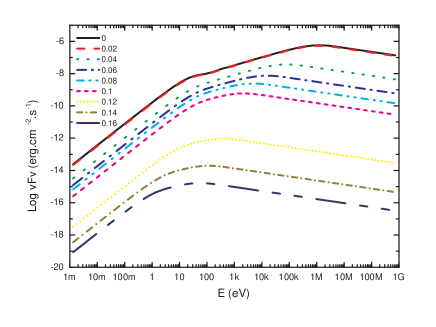
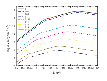
Our numerical results have been shown in Fig.1 and Fig.2. We choose $\theta_{\rm j}=0.1$, $\theta_{\rm c}=0.02$, $\gamma_{0}=500$, $r_{\rm d}=4.0\times 10^{16}{\rm cm}$, $d_{\rm L}=1\times 10^{28}{\rm cm}$, $\epsilon_{\rm e}=0.1$, $\epsilon_{\rm B}=0.1$, $p=2.5$, $k=2$ for a nonuniform jet and $k=0$ for an uniform one.

It seems that for a nonuniform jet, the spectra and fluxes fit both GRBs and XRFs observations fairly well. Viewed from the center, $E_{\rm p}$ is about $100{\rm KeV}\sim 1{\rm MeV}$, and flux is about $10^{-7\sim-6}{\rm erg}\cdot{\rm cm}^{-2}\cdot{\rm s}^{-1}$, these are the typical values for GRBs(e.g. in Fig.1, the cases for $\theta_{\rm v}=0,0.02,0.04$). While when viewed from off-axis, $E_{\rm p}$ is about $10{\rm KeV}-100{\rm KeV}$, flux is about $10^{-8\sim-7}{\rm erg}\cdot{\rm cm}^{-2}{\rm s}^{-1}$(e.g. in Fig.1, the cases for $\theta_{\rm v}=0.04,0.06$), these are the typical values for XRFs. When $\theta_{\rm v}=0.08,0.1$, $E_{\rm p}$ is about a few KeV, the flux seems a little lower, but still can be detected if the source distance is not so large.

But it seems that for an uniform jet, the flux from the jet edge, where XRFs are thought to be from in this model, are too low. In this case the spectra peak at 10-100KeV, the fluxes are about $10^{-13\sim-10}{\rm erg}\cdot{\rm cm}^{-2}{\rm s}^{-1}$(e.g. in Fig.2, the cases for $\theta_{\rm v}=0.105,0.11,0.12$). It can only explain nearby XRFs, such as $z\leq 0.2$(Yamazaki et al. 2002). But XRFs are more likely have cosmological origins(Heise 2002).

Figure 3: A spectrum and flux fit to XRF971019 using our calculation program. Here we chose $\theta_{\rm j}=0.1$, $\theta_{\rm c}=0.02$, $\gamma_{0}=500$, $\theta_{\rm v}=0.08$, $p=5.4$, $r_{\rm d}=4.0\times 10^{15}{\rm cm}$, $d_{\rm L}=4.2\times 10^{26}{\rm cm}\sim 136{\rm Mpc}$.

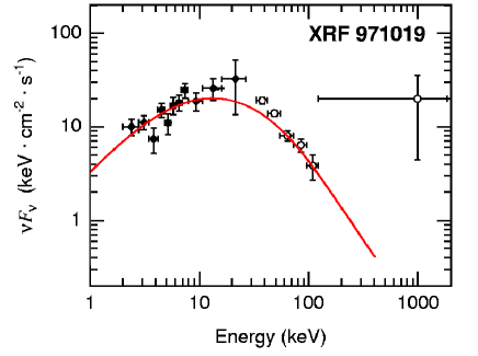
Fig.3 is a fit to the most significant X-ray flash XRF971019 using our nonuniform jet model. Here we choose $p=5.4$ because the high $\nu F_{\nu}$ power law index is about -1.7. This value seems a little unusual, but similar to the case of GRB980425 whose high-energy power-law photo index is $3.8\pm 0.7$(Galama et al. 1998). XRF is defined as X-ray transients with duration less than $1000{\rm s}$ which is detected by WFC(on BeppoSAX) but not triggered GRBM(on BeppoSAX). Actually, this definition may lead to strong selection effects on those transients with high power law index.

We assume that every explosion has same luminosity and jet shape, luminosity at center is $L_{\nu}(0)$, and at viewing angle $\theta$ is $L_{\nu}(\theta)=L_{\nu}(0)(\theta/\theta_{\rm c})^{-2k_{1}}$. Depending on the viewing angle $\theta$, a burst can be detected only at the distance $D(\theta)$:

$$D(\theta)\leq D_{\rm max}(\theta)=(\frac{L_{\nu}(0)(\theta/\theta_{\rm c})^{-2k_{1}}}{4\pi F_{\nu,{\rm min}}})^{1/2}$$ (15)

Here $F_{\nu,{\rm min}}$ is the threshold of a detector. So the numbers of GRBs($N_{\rm GRBs}$) and XRFs($N_{\rm XRFs}$) are:

$$N_{\rm GRBs}=\int_{0}^{\theta_{\rm c}}\frac{4}{3}\pi D(\theta_{\rm c})^{3}n\frac{\sin(\theta)d\theta}{2}$$

$$+\int_{\theta_{\rm c}}^{\theta_{\rm cr}}\frac{4}{3}\pi D(\theta)^{3}n\frac{\sin(\theta)d\theta}{2}$$

$$N_{\rm XRFs}=\int_{\theta_{\rm cr}}^{\theta_{\rm j}}\frac{4}{3}\pi D(\theta)^{3}n\frac{\sin(\theta)d\theta}{2}$$

$n$ is the number of bursts per unit volume, $\theta_{\rm cr}$ is the critical angle, if viewing angle is larger than it the explosion will be observed as XRFs. We assume the peak energy from the jet axis $E_{\rm p,c}=1{\rm MeV}$, here we divide XRFs from GRBs with $E_{\rm p}=90{\rm KeV}$, then the critical angle $\theta_{\rm cr}=(\frac{E_{\rm p,c}}{90\rm KeV})^{\frac{1}{4k_{1}}}\theta_{\rm c}$. We get:

$$\frac{N_{\rm GRBs}}{N_{\rm XRFs}}=\frac{\frac{3}{2}\theta_{\rm c}^{-1}-\theta_{\rm cr}^{-1}}{\theta_{\rm cr}^{-1}-\theta_{\rm j}^{-1}}\sim 2.6$$ (16)

This result depends on the parameters we have chosen. Changing these parameters in a reasonable range will change this result a little but not much. On the other hand, these parameters can be restricted by observed ratio.

4 Discussion and conclusion

It is more likely a gamma-ray burst outflow is jetted. The energy distributions are more likely smoothly deducing with angle distance from the center than uniform in the cone. In this paper, we use a structured jet model which the energy per unit solid angle decreasing as $\epsilon(\theta)\propto\theta^{-k}$. We reproduce the key observational features of XRFs and GRBs. Our calculations are based on the external shock model which seems not ideal for reproducing GRBs with highly variable temporal structure, but still adapt to those bursts with smooth light curves. And our calculations should also adapt to the internal shock model.

We have chosen $\theta_{\rm c}=0.02$ and $\gamma(0)=500$ in our numerical calculations. But the lower limit to $\theta_{\rm c}$ is about $1/\gamma_{\rm max}\sim 10^{-3}$, and the bulk Lorentz factor in the center have an maximum value to $\gamma_{\rm max}\sim 10^{5}$(Piran 1999; Rossi et al. 2002). Thus $E_{\rm p}$ may be in excess of MeV when the axis just point towards us though the probability for this case is small.

We take $k=2$ for a nonuniform jet, Rossi et al. had shown that $1.5\leq k\leq 2.2$ is the reasonable value for fitting observations well(Rossi et al. 2002; Zhang & Meszaros 2002a). For the cases of $1\leq k\leq 3$, the calculated spectra and fluxes, also the relation between $E_{\rm p}$ and $L$ are similar to that of $k=2$. Because of beaming effect and shape of equal arrival time surface, the radiation mainly comes from outflows just pointing towards observer. We will observe a similar spectrum and flux at a larger(smaller) viewing angle when $k$ is smaller(larger). But it will change our solutions of GRBs to XRFs observational ratio. We also assume $k_{1}=k_{2}=1$ in the calculations through this paper, $k_{1}\neq k_{2}$ is a more complex case which may lead to very complicated calculation.

We find that the observational ratio of GRBs to XRFs is about several in our model. It predicts that more XRFs or soft GRBs will be found in the future when more sensitive instruments are launched. Barraud et al. have presented 35 GRBs/XRFs spectra from HETE-2 whose band is 4-700KeV(Barraud et al. 2003), the numbers of bursts with $E_{\rm p}$ higher and lower than 90KeV in these 35 GRBs/XRFs are 24 and 11, similar to our calculated result 2.6.

The observation had shown a correlation $E_{\rm p}\propto L^{1/2}$(Lloyd et al. 2000; Amati et al. 2002; Wei & Gao 2003). This result is still not well explained except for some arguments based on some very simple assumption(Lloyd et al. 2000). We find in our model, for a single explosion viewed from different angles, $E_{\rm p}\propto L^{2/3}$, close to the observational relation. For a dirty fireball the relation between initial Lorentz factor and explosion energy is uncertain. If simply assuming that $\Gamma\propto L^{1/6}$, it leads to the same conclusion we have presented.

Our model cannot be distinguished from a dirty fireball model just by a single X-ray flash, but for these two models the statistical properties such as the observational ratio of GRBs to XRFs are different. In addition, the structured jet model is also different from a dirty fireball in their afterglows. A very obvious feature for a structured jet is that when $\theta_{\rm v}/\theta_{\rm c}$ and $k$ is large, there will be a prominent flattening in the afterglow light curve, and a very sharp break occurring at the time $\gamma\sim(\theta_{\rm v}+\theta_{\rm c})^{-1}$ after the flattening(Rossi et al. 2002; Wei & Jin 2003). We suggest that such features are more likely to be found in an X-ray flash afterglow rather than in a gamma-ray burst afterglow if an XRF does come from an off-axis nonuniform jet, because an XRF has a larger $\theta_{\rm v}/\theta_{\rm c}$ value than a GRB in this model.

Orphan afterglows once caused great expectations to testify GRB collimation(Rhoads 1997). In a nonuniform jet, orphan afterglows may be generated in two ways. One way is when viewing angle is out of the jet edge(e.g. in Fig.1 the cases $\theta_{\rm v}=0.12,0.14,0.16$, the fluxes will increase to detectable values at later time). In this case, the GRBs/XRFs are undetectable due to beaming effect but afterglows are detectable which are less beamed. The other probable way is that the Lorentz factor along the line of sight is sufficiently small that the peak energy $E_{\rm p}$ is below the X-ray band. This case did not appear in our calculations, it will appear if we choose a smaller value of $\theta_{\rm c}/\theta_{\rm j}$ or a larger value of $k_{1}$.

We have neglected the evolution of bulk Lorentz factor and lateral expansion of the jet which would make the calculations more complex and we think these effects are not very important before outflows arrive at their deceleration radius. Huang et al. have given out an overall evolution of jetted gamma-ray bursts in detail(Huang et al. 2000), we suggest that one should take all these effects into account for more realistic calculations.