A brief (blazar oriented) overview on topics for multi-wavelength observations with
TeV photons

Abstract

Multi-wavelength observations with TeV photons are an essential diagnostic tool to study the physics of TeV sources. The X-ray and optical bands are especially valuable, since they sample TeV energy electrons and their most effective seed photons for the inverse Compton up-scattering. The complex variability of blazars, however (timescales from years down to minutes, with different patterns and SED behaviours), requires a great effort on simultaneous campaigns, which should be performed possibly over several days. Most important is the possibility to have spectra in all the three bands: with the new instruments, both in TeV and X-ray bands, this has become now feasible on timescales less than one hour. The insights from such observations can be tremendous, since recent results have shown that the X-ray and TeV emissions do not always follow the same behaviour, and flares can have different relations between rise and decay times. Unfortunately, the strong pointing constraints of XMM do not allow the full use of this satellite simultaneously with ground telescopes.

1 Introduction

With the upcoming of the new generation of Čerenkov Telescopes (CT, e.g. H.E.S.S., VERITAS, CANGAROO III, MAGIC), TeV astronomy is about to greatly improve its scientific capabilities. Multi-wavelength observations are an essential tool to investigate how TeV sources work. Below, I will briefly present some recent topics and perspectives for multi-wavelength observations with TeV photons, with main emphasis on blazars since they represent nearly all the extragalactic sources so far detected. The scheme is the following: at first I will very briefly recall different mechanisms to produce TeV photons, to identify the most interesting frequencies to accompany TeV observations. Then I will discuss the objects’ main variability characteristics, which determine the observation strategies, and will focus on some issues related to the simultaneous coverage.

2 TeV emission ingredients

The first obvious requirement to produce TeV photons is to have particles with TeV energies, for energy conservation. According to which particle is the main carrier of this energy, the recipes for TeV emission can be divided in two classes. In the so called “hadronic” models, protons play the main role, producing TeV photons through hadronic interactions (as $pp\to\pi^{0}\to 2\gamma$ pohl , or $p\gamma\to\pi\to\gamma e^{+}e^{-}$ with a subsequent electromagnetic cascade mann ), or directly through synchrotron radiation in strong magnetic fields (B$\sim$100G), with emission at lower frequencies contributed also by secondary pair-produced electrons ahap . For these models the overall spectral energy distribution (SED) is determined by the details of the cascade or the secondary electrons production, as well as the initial particle spectrum and source conditions, so that basically all lower frequencies are equally interesting to distinguish among them and to constrain the physical parameters.

In the “leptonic” models, instead, electrons are the main particles, producing TeV photons through the inverse Compton (IC) process (more economic than the synchrotron one). Allowing for beaming effects, to give origin to an observed TeV photon (i.e. a TeV/$\delta$ photon in the comoving frame), an electron needs at least an energy $\gamma m_{e}c^{2}\geq{\rm TeV}/\delta$ (i.e. $\gamma\geq 10^{5}$ for $\delta\sim 10$). The seed photons most effective to be up-scattered by these electrons are of frequency $h\nu\leq m_{e}c^{2}/\gamma$ (in the co-moving frame), since above they scatter in the Klein-Nishina regime. In the presence of magnetic field, these same electrons will also produce synchrotron radiation of observed energy $h\nu=1.5B({\rm Gauss})(\gamma/10^{5})^{2}(\delta/10)$ keV. In this scenario, therefore, two other frequency bands stand out in a natural way: the X-ray one, which can provide number density and energy distribution of the electrons also emitting in the TeV band, and the “optical” one (in a broad sense, i.e. from UV to IR), where we can have information about the most effective seed photons. Multi-wavelength observations in these three bands represent therefore a powerful diagnostic tool for the acceleration mechanism and the details of the high energy emission (as well as a test for the leptonic scenario itself).

Note anyway that, whatever scenario is adopted, the conditions must be compatible with the TeV photons survival (since we detect them), i.e. the source must be transparent with respect to the $\gamma$-$\gamma$ absorption.

Figure 1: Lightcurves of Mkn 501 in X-rays, revealing three very different variability timescales: years, days, minutes. Left: 7–day weighted averages of RXTE ASM data. Center: ASCA long observation ($\sim$10 days) on March 2000, 6000s bins chiharu . The spectrum hardens during flares (see the different soft and hard countrate). Right: XTE PCA observation on 25/5/98, 96s bins catanese . After UTC 18.3, the spectrum hardened from $\alpha=1.02$ to $\alpha=0.87$ ($\pm 0.03$).

3 Variability properties

Multi-wavelength observations of variable sources require an understanding of their variability characteristics to decide the best observing strategy. The most variable and potentially strong extragalactic sources of TeV photons are Gamma-Ray Bursts (GRBs) and blazars. For GRBs (whose flux decays as $\sim t^{-1}$) the choice is rather straightforward (albeit difficult to carry out): to observe as quick as possible and until it fades away.

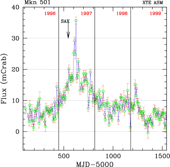
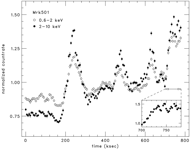
Blazars instead are characterized by very different variability timescales, from years to minutes, and not only among different objects but also in the single sources. In high energy peaked BL Lacs (HBLs, which comprise all the detected TeV sources) we are now aware of at least 3 main timescales, well exemplified by the Mkn 501 behaviour in X-rays (Fig. 1): a long-term one, from months to years (e.g. the 1997 huge flare); a “middle-term” one, with a typical timescale of $\sim$1 day (as revealed by the ASCA long observations, also in Mkn 421 and PKS 2155-304 chiharu ); and a short-term one, from hours down to even minutes, as observed by RXTE in May 1998, with a hard X-ray doubling timescale of $\sim$6 minutes catanese . Extremely short variability is also a property of the TeV emission (e.g. Mkn 421, gaidos ; aha2 ), with doubling timescales as short as 20 minutes.

Figure 2: SEDs of four HBLs, showing two characteristic “flaring modes” for the synchrotron peak. Left (Mkn 421, PKS 2155-304): as the flux varies, the peak energy remains nearly stable. Right (Mkn 501, 1ES 1959+650): as the flux increases, the peak shifts at high energies, with a pivoting in the optical–soft-X band. For 1ES 1959+650 during the May 2002 flare, the pivoting is inferred by the high X-ray flux and hard spectrum ($\alpha\approx 0.6$, henric ) and the contemporaneous optical upper limit (MERCATOR telescope; details in horn19 ). See henric for the results of the multi-wavelength campaign.

Figure 3: Left: SED of 1ES 1426+428 costa1 . The upper TeV data correspond to the absorption corrected ones (using the Primack EBL model, costa2 ). This source is characterized by large peak shifts not coupled with large flux variations, as opposed to Mkn 501 (see right). Right: historical X-ray data. The peak frequency is determined by curved or broken power-law best fits, with upper and lower limits given by the X-ray spectrum being steeper or harder than 1, respectively, over the whole instrument’s band.

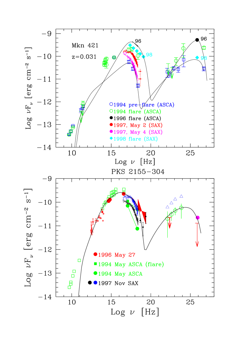
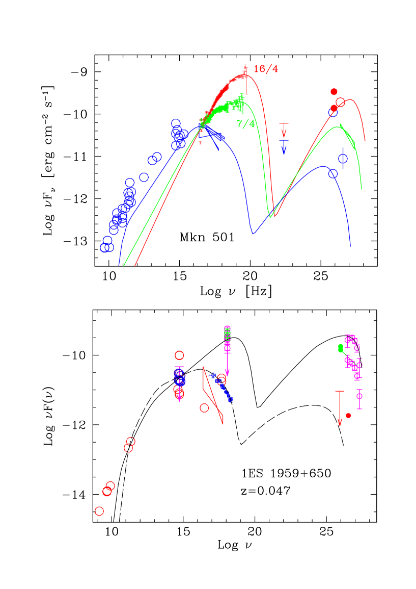
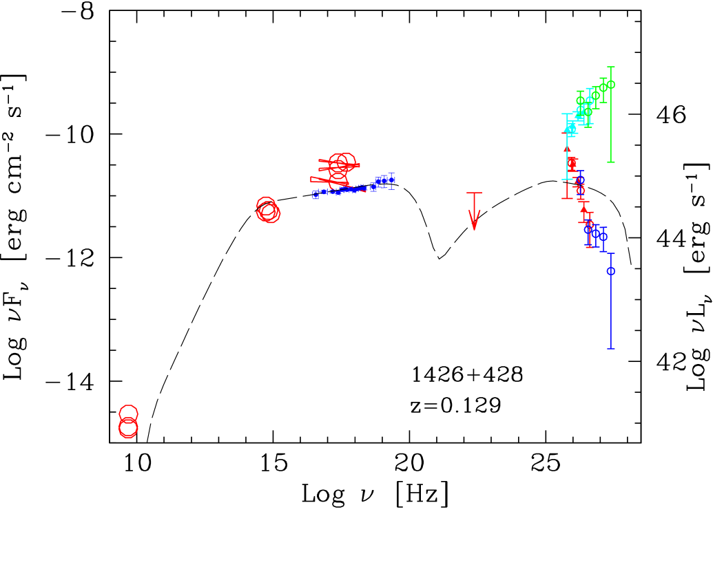
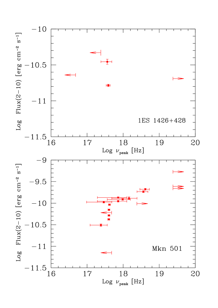
Connected with the flux variability, HBLs show also strong spectral variations, which often change the position of the SED peaks. Although there seems to be a trend (in the X-ray and TeV bands) for “harder when brighter” spectra, there is not a unique relation between flares and (synchrotron) peak changes. In fact, we can outline 3 types of behaviour: a “Mkn421–like” one (Fig. 2 left), where the peak frequency changes very little despite large flux variations gfoss ; a “Mkn501–like” one (Fig. 2 right), where during flares the peak shifts towards higher energies by orders of magnitude (e.g from $<$1 to $\geq$100 keV); and a “1ES 1426+428–like” one (Fig. 3), which seems characterized by large peak variations (of the same magnitude of Mkn501) but during roughly constant flux states (at least in the X-ray band). A “Mkn501–like” behaviour has been recently followed by 1ES 1959+650 during the May 2002 strong flare henric , with striking similarities also in the ’pivoting’ of the SED around the optical–soft-X range horn19 .

All these differences and similarities suggest that there are common but intrinsically different parameters/mechanisms driving the variability, whose understanding requires to follow the overall SED changes on all typical timescales.

4 The X-ray–TeV connection

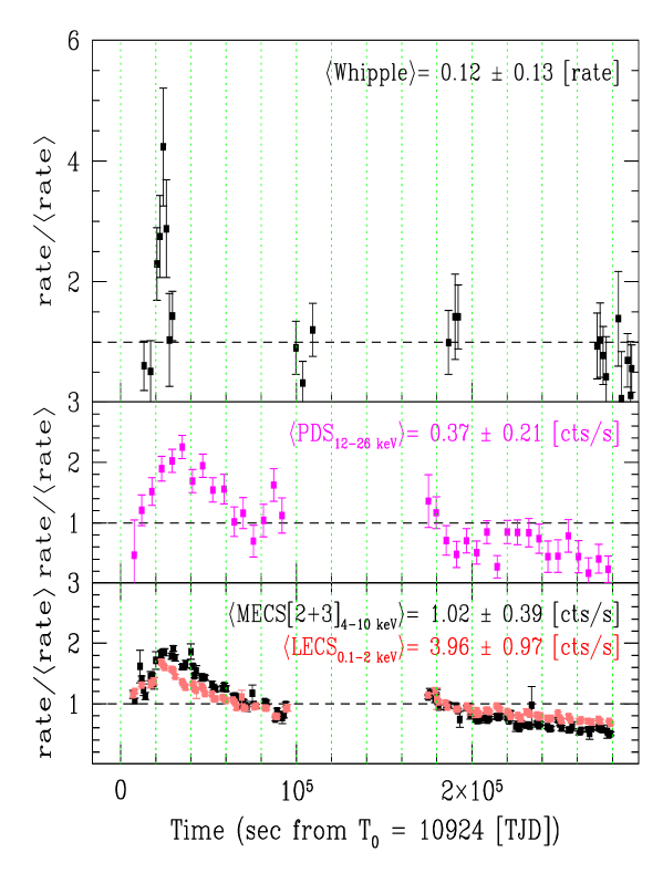
The interest of X-ray and TeV observations is that they sample electrons of roughly equal energy, emitting through two different processes. In HBLs, moreover, the bulk of the luminosity is emitted in those bands and it appears to be produced by the same electron population, as suggested by the often observed tight correlation between the two emissions. A strong confirmation of this last hypothesis has come from a simultaneous observation of Mkn 421 in 1998 (Fig. 4), where the peaks of the emissions were correlated within one hour (although with different halving times; maraschi ).

Figure 4: Left: simultaneous lightcurves of Mkn 421 by WHIPPLE ($>2$TeV) and BeppoSAX , in April 1998 maraschi . Right: a simultaneous one week monitoring of Mkn 421 by RXTE (PCA) and HEGRA, in March 2001 horns421 .

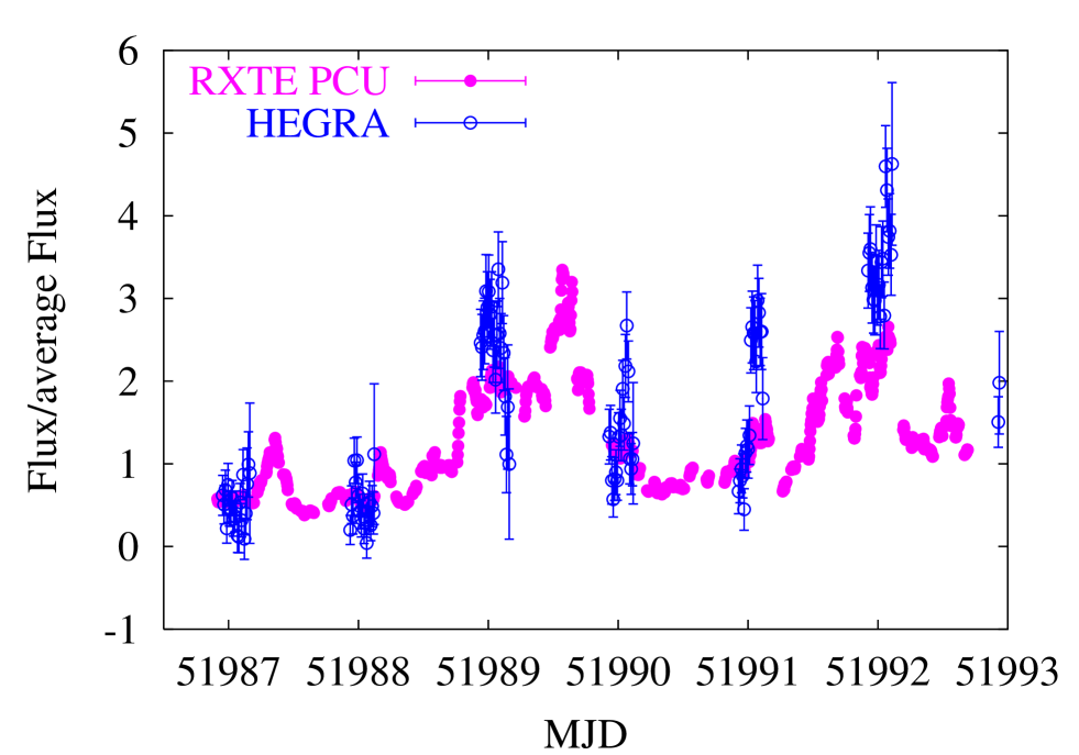
However, new results are now showing that this relation may be more complex than expected, since the two bands does not always follow the same behaviour. An example is given again by Mkn 421, in 2001 (Fig. 4 right): although there is a general correlation, there are periods where we see a strong decrease (MJD $\sim$51989) or a rapid flare (MJD $\sim$51990) of the TeV flux not accompanied by relevant changes in the X-ray band. This behaviour seems also confirmed by 1ES 1959+650 in its 2002 active state, where evidence was found for a so called “orphan” $\gamma$-ray flare (i.e. not accompanied by an X-ray flare) henric . More observations, possibly over several days, are necessary, to see if there are also X-ray flares not accompanied by TeV flares, and to unveil possible lags between them and with the seed photons fluxes.

Figure 5: Two intra-night flares of Mkn 421 at TeV energies (HEGRA data, taken on two consecutive nights), showing different rise and decay timescales aha2 . Below, the hardness ratio is reported (calculated from the bands 0.75–1.5 and 1.5–4.0 TeV).

For both diagnostics and model testing, the intra-day activity of TeV blazars is perhaps the most challenging, since the shortest TeV timescales pose the tightest constraints to the size of the emitting region and to the $\gamma$-$\gamma$ transparency celotti . Moreover, recent HEGRA data on Mkn 421 have shown an entire “zoo” of flares with quite different rise and decay times (e.g. Fig. 5), hint of a complex interplay between acceleration and cooling/escape times. The improvement in sensitivity ($\sim$1 order of magnitude) of the new generation CT, coupled with the continuous coverage provided by the large area X-ray telescopes (CHANDRA, XMM), are now making possible to follow the spectral evolution in both bands on hour timescales and without gaps, allowing to study the inner jet conditions with unprecedented detail.

Another fundamental advantage of the new generation CT is their lower energy thresholds ($\leq$150 GeV), which will provide data also at energies not (or less) affected by absorption due to $\gamma$-$\gamma$ collisions with the cosmic Extragalactic Background Light (EBL, steck ; primack ). Together with the study of the correlated X-ray–TeV variability, from simultaneous observations we hope to be able to constrain the whole SED model parameters such to “measure” the EBL by comparing the predicted intrinsic TeV spectrum with the observed one coppi ; kraw .

Figure 6: Left: sky visibility plots for XMM and CHANDRA (from the respective handbooks). Right: visibility of PKS 2155-304 by H.E.S.S. during 2004, above a certain altitude (in degrees). The nearly horizontal stripes correspond to the moonlight–contaminated nights, i.e. not usable by CTs. For simultaneous observations, while the CHANDRA window goes from April to end December, the XMM one is limited to 28/4–27/5 and 31/10–26/11.

5 Observation strategies

It is clear at this point that we need simultaneous observations in all the three main bands with spectral information. Spectra are precious also in the “optical” band, to outline the overall SED shape (and peak position) and to follow its evolution during flares. The “optical” band is important also because changes in the seed photons flux or/and spectrum may give origin to different behaviours between the TeV and X-ray emissions.

The ’long-term’ variability requires of course a long term monitoring program of a number of objects (as now done by RXTE ASM), which should continue to be done preferably at X-rays, since an only optical monitor would have missed the “Mkn501-like” flares, due to the pivoting of the SED at low frequencies. Simultaneous campaigns over several days, maximizing the continuous coverage through the coordination of ground CT and optical telescopes, will allow instead to sample both the middle and short-term variabilities, and to reveal possible lags. Long observations will allow also to investigate the relations between these two variabilities, e.g. if the shortest one appears only on top of the other or not, and if with different characteristics. For the same reason, simultaneous campaigns should be performed not only during the flares detected by the long term monitoring, but also in quiescent periods.

6 A warning about X-ray coverage

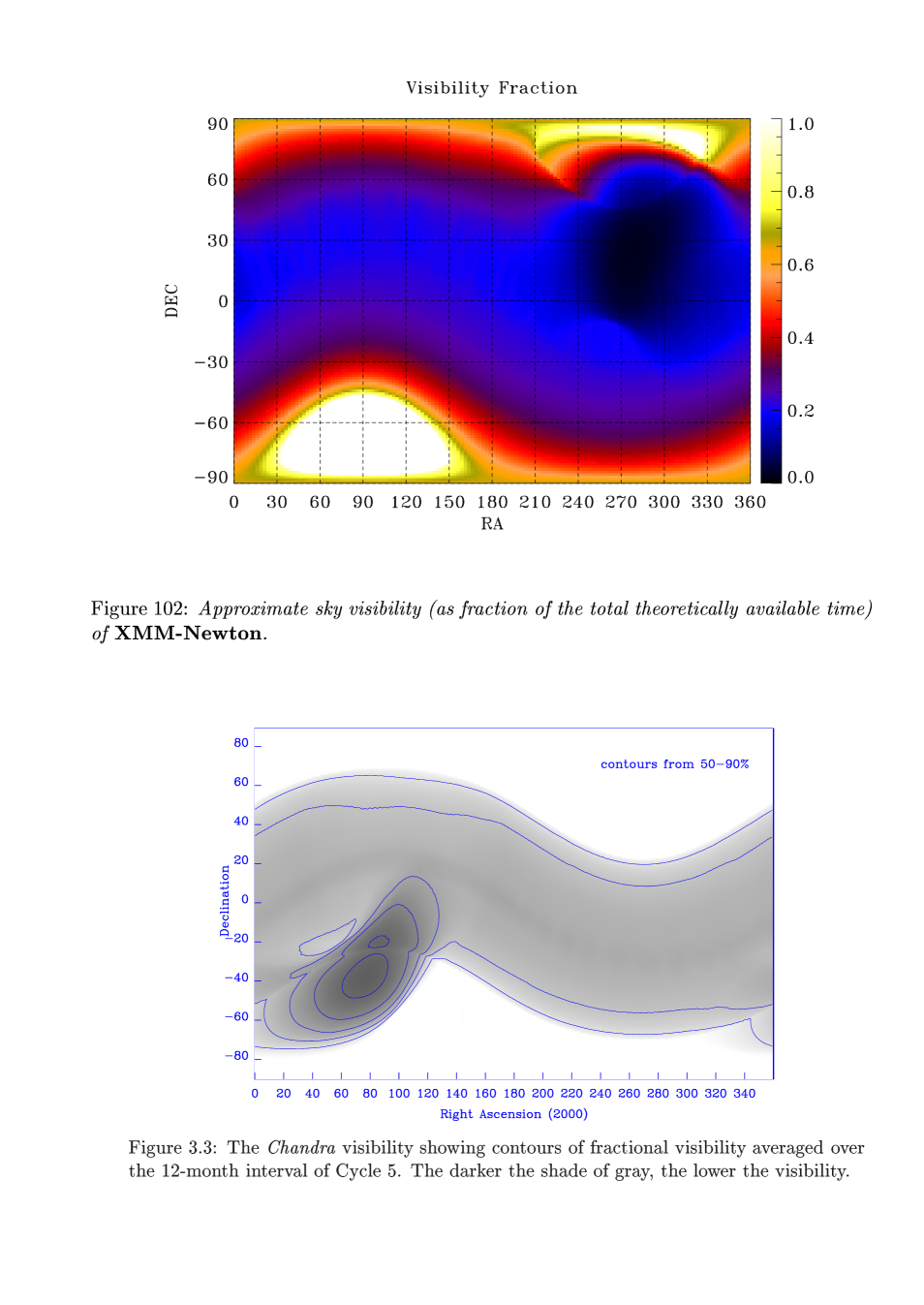
Together with CHANDRA, XMM is in principle the best X-ray instrument for this type of studies, thanks to its large collecting area (providing spectra on shorter timescales) and its long orbital period, which allows for continuous observations without gaps up to $\sim$37 hrs. Regrettably, the strong constraints on the solar panels orientation (the sun avoidance angle has to be $70^{\circ}\leq\theta\leq 110^{\circ}$) severely affects the satellite performance in two for us important areas: the ability to perform observations triggered by flaring states and simultaneously with ground telescopes. As shown in Fig. 6 (left), the visibility of an object during the year is limited for most of the sky to $\sim$2-3 months, with correspondingly low probability that a flare will occur in the right epoch. Even more important, the constraints involve also the anti-solar direction (contrary to CHANDRA), thus making impossible to observe a source when it is visible under the best conditions from ground telescopes (i.e. for the full night).

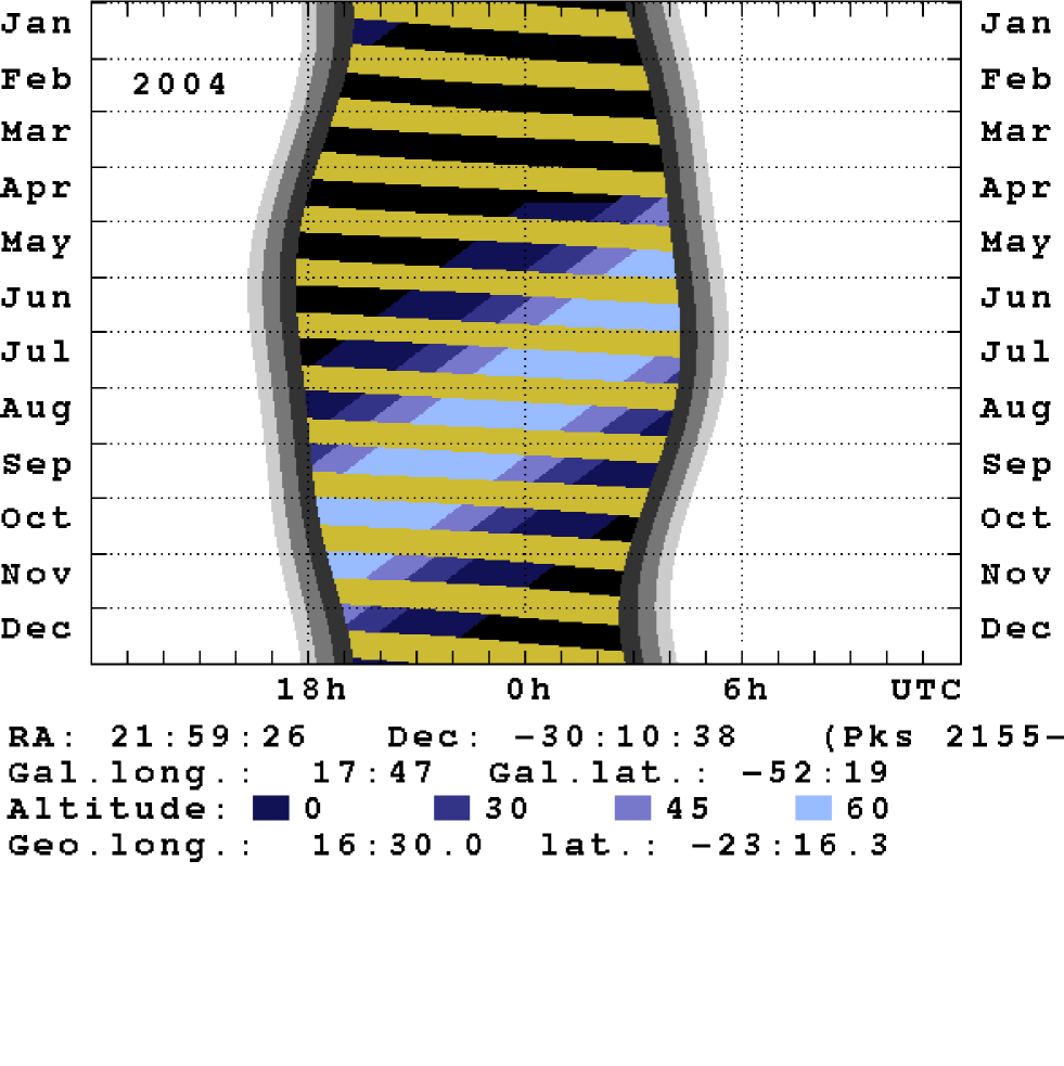
An example is given by PKS 2155-304 with H.E.S.S. (Fig. 6, right): the source can be pointed by XMM only in May (28/4–27/5) and November (31/10–26/11), i.e. when it can be observed by H.E.S.S. for only $\sim 2$ hours at the end or beginning of the night. The same problems affect also INTEGRAL, although with slightly less constraints on the sun angle and thanks to the wide field of view of its instruments (JEM-X f.o.v. is 4.8^∘, fully coded). Since SWIFT will be devoted mainly to GRBs studies (but see gehrels for its possible use also with flaring blazars), this leaves the TeV community for the next years (i.e. when the new generation CTs are becoming operative) with only CHANDRA and RXTE as the main X-ray satellites for simultaneous campaigns.

References

- (1) Aharonian F.A. 2000, New A, 5, 377
- (2) Aharonian F.A et al. 2002, A&A, 393, 89
- (3) Catanese M. & Sambruna R., 2000, ApJ, 534L, 39
- (4) Costamante L. et al., 2001, A&A, 371, 512
- (5) Costamante L. et al. 2003, proc. Relativistic jets in the Chandra and XMM era, Bologna 2002 (astro-ph/0301211)
- (6) Celotti A. et al., 1998, MNRAS, 293, 239
- (7) Coppi P.S. & Aharonian F. A., 1999, ApJ, 521, L33
- (8) Fossati et al., 2000, ApJ, 541, 166; and these proceedings
- (9) Gaidos J.A. et al., 1996, Nature, 383, 319
- (10) Gehrels N., these proceedings
- (11) Horns et al., 2003, proc. High Energy Blazar astronomy, Turku 2002, (astro–ph/0209454)
- (12) Horns et al., 2003, proc. The Universe viewed in Gamma-Rays, Kashiwa 2002
- (13) Krawczynski H. et al., 2002, MNRAS, 336, 721
- (14) Krawczynski H. et al., these proceedings
- (15) Mannheim K. 1993, Science, 279, 684
- (16) Maraschi L. et al., 1999, ApJL, 526, 81
- (17) Pohl M. & Schlickeiser R., 2000, A&A, 354, 395
- (18) Primack et al., 2001, AIP Conf. Proc. 558, 463
- (19) Stecker F.W. et al., 1996, ApJ, 473, L75
- (20) Tanihata et al. 2001, ApJ, 563, 569