IRAS  PSCz v.s. IRAS  1.2-Jy Model Velocity Fields: A Spherical Harmonics Comparison.

Abstract

We have used the two IRAS redshift surveys, 1.2-Jy (Fisher et al. 1995) and PSCz (Saunders et al. 2000), to model the linear velocity fields within a redshift of 8 000  km s^-1 and have compared them in redshift space. The two velocity fields only differ significantly in their monopole components. The monopole discrepancy cannot be solely ascribed to shot-noise errors and incomplete sky coverage. The mismatch seems to arise from incompleteness of the PSCz catalog at fluxes $\leq$ 1.2 Jy. The 1.2-Jy and PSCz higher order velocity multipoles, particularly the dipole and quadrupole components, appear to be consistent, suggesting that the dipole residuals found by Davis, Nusser and Willick (1996) when comparing 1.2-Jy and Mark III velocity fields probably originates from the Mark III velocities calibration procedure rather than from uncertainties in the model velocity field. Our results illustrate the efficiency of the spherical harmonics decomposition techniques in detecting possible differences between real and model velocity fields. Similar analyses shall prove to be very useful in the future to test the reliability of next generation model velocity fields derived from new redshift catalogs like 2dFGRS (Colless et al. 2001), SDSS (York et al. 2000), 6dF and 2MRS.

1 Introduction

In the framework of linear gravitational instability theory and linear biasing a comparison between the predicted and observed peculiar velocities allows us to measure the so called $\beta$ parameter

$$\beta\equiv\frac{\Omega_{m}^{0.6}}{b}.$$ (1)

i.e. a combination of the mass density parameter, $\Omega_{m}$, and the linear bias parameter, $b$, which relates the mass overdensity field $\delta$ to the density fluctuations in galaxy counts $\delta_{g}$, through $\delta_{g}=b\delta$. Several different techniques have been used to compare measured peculiar velocities (taken from all available catalogs: Mark III Willick 1997a, SFI Haynes 1999, ENEAR da Costa et al. 2000, SEcat Zaroubi 2002) to predict velocities that, in most cases, have been obtained from two redshift surveys of IRAS galaxies: the 1.2-Jy and the PSCz catalogs.

Most analyses have investigated the consistency between model and observed velocities, while only a few of them have been devoted in comparing different datasets or in studying the consistency of model velocity fields. All recent works show a general consistency between models and data (Willick et al.  1997, hereafter WSDK; Willick and Strauss 1998; Sigad et al. 1998; Dekel et al. 1999; Branchini et al. 1999, hereafter B99; Nusser et al. 2000; Zaroubi et al. 2002) with one noticeable exception represented by the work of Davis, Nusser & Willick (1996, hereafter DNW). Their analysis showed that the velocity residuals between the Mark III peculiar velocities and the 1.2-Jy predictions display a significant spatial correlation. Subsequent analyses by WSDK and Willick and Strauss (1998) were performed using the same dataset, a similar model velocity field but a different comparison technique, called VELMOD, which allows for independent calibrations of Mark III velocities in each of the Mark III sub-catalogs. As a result the observed and model velocity fields were brought into better agreement, at least within a redshift distance $s=7\,500$ km s^-1 and returned a calibration inconsistent with the original one performed by Willick et al. (1997a).

While these results suggest that the DNW mismatch originates from calibration problems in the Mark III catalog, the possibility that systematic errors in the 1.2-Jy model velocities also contribute to the discrepancy has been completely overlooked. In particular, we ignored whether the velocity fields predicted from the deeper IRAS PSCz catalog provides a better match to the Mark III velocities than the shallower 1.2-Jy catalog, considered by DNW.

The main goal of this work is to check whether the discrepancies between the 1.2-Jy and Mark III velocities can be ascribed, at least to some extent, to model uncertainties. For this purpose we compare both the overdensity and the radial velocity fields modeled from the redshift space distribution of 1.2-Jy and PSCz galaxies. This work is meant to stress the usefulness of spherical harmonics decomposition techniques in assessing the adequacy of a model velocity (or density) field through velocity-velocity (or density-density) comparisons.

In § 2 we describe how to compare velocity and overdensity fields inferred from different redshift surveys. The galaxy redshift catalogs used in our analyses are described in § 3. In sections 4 and 5 we analyse the two model overdensity fields and radial velocity fields. Our main results are discussed in § 6 and our main conclusions are presented in § 7.

2 Spherical Harmonic Coefficients Decomposition

The relations between an arbitrary scalar field $\psi({\bf s})$ and the real–valued spherical harmonic coefficients $\psi_{lm}(s)$ are

$$\psi_{lm}(s)=\int\psi({\bf s}){\mathcal{Y}}_{lm}(\hat{{\bf s}})d\Omega$$ (2)

$$\psi({\bf s})=\sum_{l=0}^{\infty}\sum_{m=-l}^{l}\psi_{lm}(s){\mathcal{Y}}_{lm}({\hat{\bf s}}),$$ (3)

where ${\mathcal{Y}}_{lm}(\hat{{\bf s}})\{l=0,..,\infty;|m|\leq l\}$ denote the well known real-valued spherical harmonics, defined as in Baker et al. (1999, hereafter BDSLS) and Bunn (1995) (see also Jackson 1999). For a given $l$ these functions are normalized to the value of ${\mathcal{Y}}_{l0}$ at the North Galactic Pole.

The amplitude of the $l$-multipole $\psi_{l}(s)$ is defined by the sum in quadrature over the $(2l+1)$-$\psi_{\,lm}$’s, where $\{m=-l,...,l\}$:

$$\psi_{l}(s)=\left[\sum_{m=-l}^{m=l}\psi^{2}_{lm}(s)\right]^{\frac{1}{2}}.$$ (4)

2.1 Peculiar velocity and overdensity fields from the distribution of galaxies in redshift space

Nusser & Davis (1994) show that in the linear regime the peculiar velocity field is irrotational not only in real space but also in redshift space and thus can be expressed as the gradient of a scalar velocity potential: ${\bf v}({\bf s})=-\nabla\Phi({\bf s})$. At a given redshift $s$, $\Phi(s)$ and $\hat{\delta}(s)$ can be expanded in spherical harmonics and related to each other through a modified Poisson equation:

$${{1}\over{s^{2}}}\left(s^{2}{\Phi_{lm}^{\prime}}\right)^{\prime}-{{1}\over{1+\beta}}{{l(l+1)\Phi_{lm}}\over{s^{2}}}={{\beta}\over{1+\beta}}\left(\hat{\delta}_{lm}-{{1}\over{s}}{{d\ln{\phi}}\over{d\ln{s}}}{{\Phi_{lm}}^{\prime}}\right),$$ (5)

where $\phi(s)$ and $\hat{\delta}_{lm}({{\bf s}})$ denote the sample selection function and the spherical components of the overdensity field, respectively. Here prime expresses $d/ds$. Solving this differential equation requires computing the redshift space density field from the observed galaxy distribution on a spherical grid using Gaussian cells of approximately equal solid angle. These cells are equally distributed in longitude (64 bins) and are centered at the Gaussian-Legendre 32 point quadrature formula in the range $-1\leq\cos(b)\leq 1$, where $b$ is the Galactic latitude. In this work we measure redshifts in the Local Group frame, and use 52 Gaussian radial redshift bins out to a distance of $s=18\,000$ km s^-1. When comparing two or more galaxy catalogs the size of the radial bin is set by requiring equal spatial resolution and the minimal shot noise constant throughout the volume. We do this setting the distance between the centers of the Gaussian cells at distance $s$ equal to the average galaxy-galaxy separation, $\sigma(s)=[\bar{n}\phi(s)]^{-1/3}$, in the sparser catalog. The mean number density is estimated as

$$\bar{n}=\frac{1}{V}\sum_{i}\frac{1}{\phi(s_{i})},$$ (6)

where the sum is over the galaxies contained within the volume $V$, which, in this work, is a sphere of radius $8\,000$ km s^-1.

Hernquist and Katz (1989) pointed out that there are two possible ways to estimate the smoothed density field: the ”scatter” and ”gather” approches. In the former approch each particle is distributed in space, and the density estimate at a given point is the superposition of individual smoothing spheres. In the latter case one defines a smoothing lenght at a given point and weights the particle in its neighborhood by the resulting kernel. The Gaussian-smoothed galaxy overdensity field at a grid cell centred around ${{\bf s}}_{n}$ is given by:

$$1+{\hat{\delta}}({\bf s}_{n})=\frac{1}{(2\pi)^{3/2}\sigma_{n}^{3}}\sum_{i}^{N}\frac{1}{\phi(s_{i})}\exp\left[-\frac{({\bf s}_{n}-{\bf s}_{i})^{2}}{2\sigma_{n}^{2}}\right],$$ (7)

where the sum is over the $N$ galaxies in the catalog, which clearly is a ”gather” approach. The smoothing width at a redshift $s$, used in this paper is $\sigma_{n}=\max[320,\sigma(s)]$  km s^-1. Since in this work we compare the PSCz catalog with the sparser 1.2-Jy catalog, we use the $\sigma_{n}$ obtained from the 1.2-Jy catalog shown in Fig. (1).

Figure 1: The 1.2-Jy smoothing width as a function of redshift. The dots represent the value of $\sigma_{n}$ at centre of the 52 redshift bins.

This smoothing scheme is tailored to keep the shot-noise uncertainty roughly constant throughout the sample volume and is similar to the optimal Wiener filtering procedure used by Lahav et al. (1994) and Fisher et al. (1995b). Moreover, the our kernel has a compact support, which simplifies the computational task.

Eqn. (5) is valid in the linear regime, where a one-to-one mapping between distance and redshift is guaranteed. This assumption is not valid in high density regions, such as cluster of galaxies, where shell crossing may occur triple valued-regions may apear. To deal with the latter effect, we adopt the same procedure as Yahil et al. (1991) and collapse the fingers of God associated with the six richest clusters in the sample listed in Table 2 of that work.

In this work we will consider galaxies within $s_{\mbox{\scriptsize{max}}}=20\,000$  km s^-1  with the spherical harmonics decomposition limited to $l_{\mbox{\scriptsize{max}}}=15$. Outlying $s_{\mbox{\scriptsize{max}}}$ galaxies are assumed to be distributed uniformly according to the mean number density of the parent catalogs.

3 Datasets

The IRAS PSCz catalog contains $\approx$ 15 500 IRAS PSC galaxies with a 60 $\mu$m flux larger than 0.6 Jy. The average depth of this survey is $\approx$ 100 $h^{-1}\,$Mpc . We restrict our analysis to a sub-sample of 11 206 galaxies within 20 000  km s^-1 from the Local Group (LG, hereafter). The areas not covered by the survey amount to 16.0% of the sky and are preferentially located near the galactic plane, in the so-called Zone of Avoidance (Saunders et al. 2000). The empty areas have been filled-in with the cloning procedure described in Branchini et al. (1999) .

The 1.2-Jy catalog (Fisher et al. 1995a) contains 5 331 IRAS galaxies with a 60 $\mu$m flux larger than 1.2-Jy within 20 000  km s^-1. This catalog has a slightly larger sky coverage of ($\approx$ 87.6$\%$) and a smaller median redshift ($\approx$ 84 $\,{\it h}^{-1}\,{\rm Mpc}$). The same B99 filling technique has been used to restore all sky coverage.

Fisher et al. (1995b) have found that uncertainties in filling-in the empty areas of the 1.2-Jy survey do not appreciably affect the spherical harmonics coefficients with $l\lesssim 15$. Similar conclusions are also valid for the IRAS PSCz survey (Teodoro et al. 1999).

The selection functions of the two surveys, that quantify the probability of a galaxy at distance $s$, have been determined as maximum-likelihood fits to the smooth function

$$\phi(s)=\left\{\begin{array}[]{ll}\left(\frac{r_{r}}{r}\right)^{2\alpha}\left(\frac{r_{\star}^{2}+r^{2}_{s}}{r_{\star}^{2}+r^{2}}\right)^{\beta}&\quad,~{}s\geq H_{0}\,r_{s},\\ 1&\mbox{\quad,~{} otherwise,}\\ \end{array}\right.$$ (8)

where $r=s/H_{0}$ is expressed in $\,{\it h}^{-1}\,{\rm Mpc}$ (Yahil et al. 1991). The best-fit parameters, determined using the galaxies within $8\,000$ km s^-1 and assuming a flat universe with $\Omega_{m}=1$, are shown in Tab. (1). The quantity $r_{s}$ in Eqn. (8) accounts for the incompleteness of faint galaxies in the innermost regions of the catalogs (Rowan-Robinson et al. 1990, Yahil et al. 1991).

Table 1: Selection function parameters for IRAS catalogs.

Catalog	$f_{\mbox{\scriptsize{$60\mu m$}}}^{\mbox{\scriptsize{lim}}}$	N${gal}^{\mbox{\,{\scriptsize{a}}}}$	$\alpha$	$\beta$	$\gamma$	$r_{s}^{\mbox{\,{\scriptsize{b}}}}$	$r_{\star}$	$\bar{n}$
	[Jy]					[$\,{\it h}^{-1}\,{\rm Mpc}$]	[$\,{\it h}^{-1}\,{\rm Mpc}$]	$[h^{3}\mbox{Mpc}^{-3}]$
PSCz	0.6	13 364	0.54	1.80	…	6.0	87.00	6.12 $\cdot 10^{-2}$
PSCz${}_{~{}0.7}$	0.7	11 170	0.57	1.80	…	6.0	76.35	6.38 $\cdot 10^{-2}$
PSCz${}_{~{}1.2}$	1.2	5 519	0.43	1.86	…	5.0	50.40	4.62 $\cdot 10^{-2}$
1.2-Jy	1.2	6 010	0.43	1.86	…	5.0	50.60	4.67 $\cdot 10^{-2}$
PSCz${}_{\mbox{\scriptsize{\,evo.}}}$ ${}^{\mbox{\,{\scriptsize{c}}}}$	0.6	13 364	0.99	3.45	1.93	6.0	76.02	5.76 $\cdot 10^{-2}$

Table 2: The parameters of the $\delta_{1.2}-\delta_{0.6}$ and $u_{1.2}-u_{0.6}$ linear regressions.

Regression	$N_{\mbox{\scriptsize{grid}}}$	$N_{\mbox{\scriptsize{dof}}}$	$A^{\mbox{\,{\scriptsize{a}}}}$	$B$	$\chi^{2}_{\mbox{\scriptsize{eff}}}/N_{\mbox{\scriptsize{dof}}}$
$\delta_{1.2}-\delta_{0.6}$	112 552	156.36	$-0.011\pm 0.014$	$1.025\pm 0.036$	0.78
$u_{1.2}-u_{0.6}$	112 552	$\lesssim$ 156.36	$60.0\pm 5.9$	$1.040\pm 0.019$	0.88

4 The IRAS PSCz and 1.2-Jy Fields Overdensity

The first step of our analysis consists of applying Eqn. (7) to compute the IRAS 1.2-Jy and PSCz overdensities onto a spherical grid of radius $18\,000$  km s^-1 and $l_{\mbox{\scriptsize{max}}}=15$ with the smoothing scheme given by Eqn. (7).

4.1 Overdensity Maps

In Figs. (2–4) we show the Aitoff projections of the PSCz (top panels) and 1.2-Jy (middle panels) galaxy overdensity fields in three spherical shells centred at $s=$ 1 000, 3 000 and 5 000 km s^-1, respectively. The thickness of each shell is defined by the Gaussian width at the distance of the shell. All maps are plotted in Galactic coordinates. The bottom panels show the map of the overdensity residuals $\delta_{\mbox{\scriptsize{res}}}(s)=\delta_{0.6}(s)-\delta_{1.2}(s)$, where the subscripts _0.6 and _1.2 refer to PSCz and 1.2-Jy surveys, respectively. In all plots the thick line indicates the zero overdensity (or residual) contour. The overdensity (residual) contour spacing $\Delta\delta$ ($\Delta\delta_{\mbox{\scriptsize{res}}}$) depends on the shell’s depth and is indicated in the Figure captions.

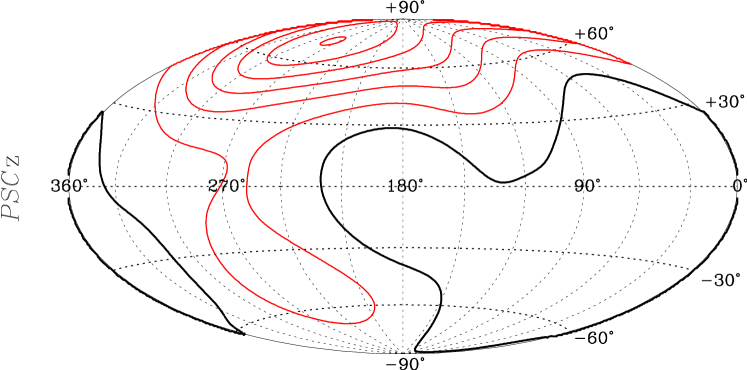
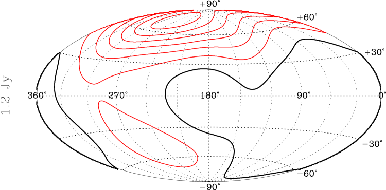
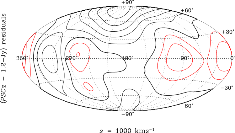
Figure 2: PSCz (top), 1.2-Jy (middle) and residual (bottom) overdensity fields in the radial shell centred at $s=1\,000$  km s^-1. The thick-line contour indicates $\delta=0$ or $\delta_{\mbox{\scriptsize{res}}}=0$ (bottom). The light- and dark-gray contours show over- and under-dense regions, respectively. In the top and middle panels the contours are equally–spaced by $\Delta\delta$ = 1.0. The bottom panel the density residuals are shown in steps of $\Delta\delta_{\mbox{\scriptsize{res}}}=0.125$.

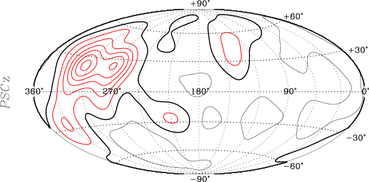
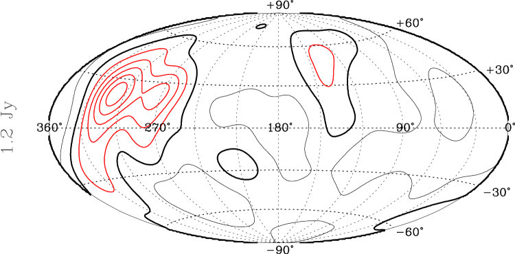
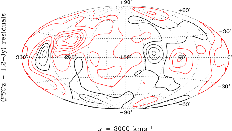
Figure 3: Same as in Fig. (2). The shell is now centred at $s=3\,000$  km s^-1 and the contour spacings are $\Delta\delta$ = 0.5 and $\Delta\delta_{\mbox{\scriptsize{res}}}=0.125$.

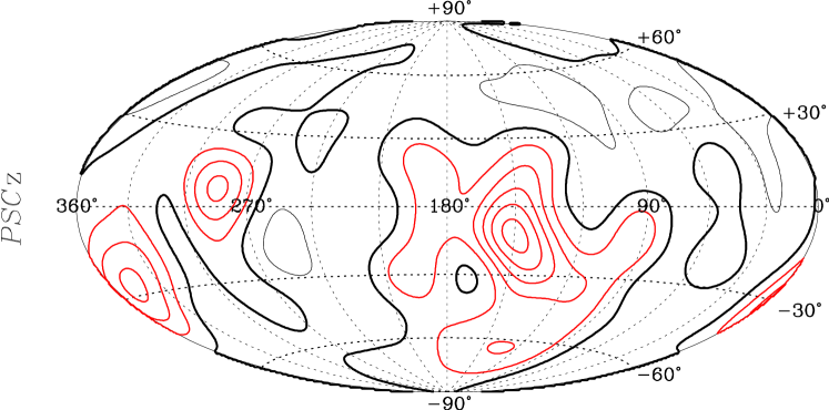
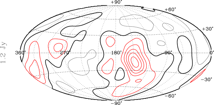
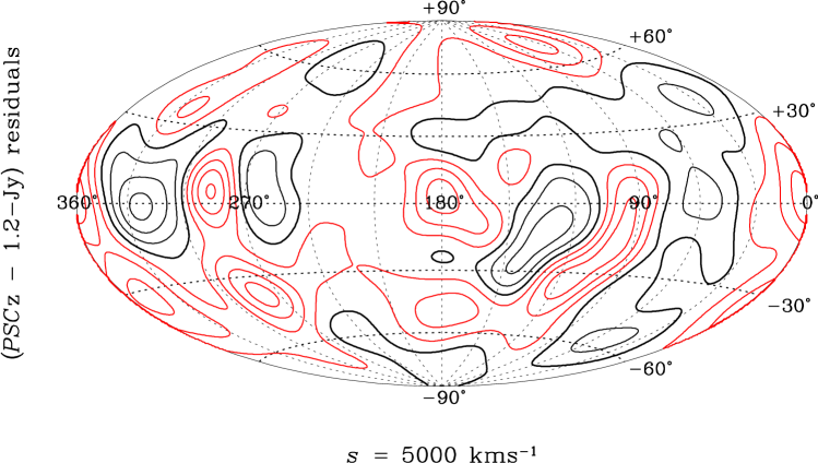
Figure 4: Same as in Fig. (2). The shell is now centred at $s=5\,000$  km s^-1 and the contour spacings are $\Delta\delta$ = 0.5 and $\Delta\delta_{\mbox{\scriptsize{res}}}=0.125$.

Detailed cosmographic studies of the structures in the nearby universe have already been performed using both the distribution of 1.2-Jy (Strauss and Willick 1995) and PSCz galaxies and will not be repeated here. We only stress that the main cosmic structures like the Virgo Cluster $(l\approx 240^{\circ},\ b\approx 75^{\circ},\ s=1000$ km s^-1$)$, the local void spanning the region $330^{\circ}\lesssim l\lesssim 120^{\circ},\ -90^{\circ}\lesssim b\lesssim 30^{\circ}$ at $s=1000$  km s^-1, the Hydra-Centaurus complex ($l\approx 270^{\circ},$ $\ b\approx 20^{\circ},\ s=3000$ km s^-1$)$ and ($l\approx 300^{\circ},\ b\approx 20^{\circ},\ s=3000$  km s^-1$)$ and the Perseus-Pisces supercluster ($l\approx 140^{\circ},\ b\approx-25^{\circ},\ s=3000$  km s^-1$)$ are detected in both surveys.

The residuals, calculated at the same gridpoints as the density fields, seem to indicate that, as expected, the largest residuals are located near the galactic plane where uncertainties in the filling-in procedure dominate the errors. In the inner shell, overdensities in the 1.2-Jy galaxy distribution appear to be larger than the PSCz ones while in the most external shell the situation is reversed.

4.2 Density Residuals

A way of quantifying possible systematic differences between the two fields is that of performing a point-to-point comparison. In absence of systematic errors we expect the two IRAS overdensity fields to be linearly related through

$$\delta_{1.2}=B\delta_{0.6}+A$$ (9)

with $A=0$ and $B=1$. $\delta_{0.6}$ and $\delta_{1.2}$ are estimated at Cartesian gridpoint positions. A zero–point offset $A\neq 0$ indicates discrepancies in the mean densities of the two catalogs while a slope $B\neq 1$ reveals the presence of systematic errors. If the values of $\delta_{0.6}$ and $\delta_{1.2}$ are independent and their errors are Gaussian then we can compute the $\chi^{2}$ statistics

$$\chi^{2}=\sum_{i=1}^{N_{\mbox{\scriptsize{grid}}}}\frac{\left(\delta_{1.2}-A-B\delta_{0.6}\right)^{2}}{\left(\sigma_{1.2}^{2}+B^{2}\sigma_{0.6}^{2}\right)},$$ (10)

where $\sigma_{0.6}$ and $\sigma_{1.2}$ indicate the typical errors in $\delta$ and ${N_{\mbox{\scriptsize{grid}}}}$ is the total number of points in the comparison. However, since the gridspacing (250 km s^-1) is smaller than the smoothing length ($\geq 320$ km s^-1), not all values of $\delta_{0.6}$ (or $\delta_{1.2}$) are independent. Indeed, the effective number of independent points used in the $\chi^{2}$ statistics, $N_{\mbox{\scriptsize{eff}}}$ is given by

$$N_{\mbox{\scriptsize{eff}}}^{-1}={N_{\mbox{\scriptsize{grid}}}}^{-2}\sum_{i=1}^{N_{\mbox{\scriptsize{grid}}}}\sum_{j=1}^{N_{\mbox{\scriptsize{grid}}}}\exp(-r_{ij}^{2}/2R^{2}_{s,i}),$$ (11)

where $r_{ij}$ is the separation between gridpoints $i$ and $j$ and $R_{s,i}$ is the smoothing radius of the Gaussian kernel at the gridpoint $i$. This expression is a generalization of Eqn. (12) in Dekel et al. (1993) to the case of a grid with variable mesh-size since $R_{s,i}$ depends on the gridpoint position. The new statistics $\chi^{2}_{\mbox{\scriptsize{eff}}}=({N_{\mbox{\scriptsize{grid}}}}/{N_{\mbox{\scriptsize{eff}}}})\chi^{2}$ is approximately distributed as a $\chi^{2}$ with $N_{\mbox{\scriptsize{dof}}}=N_{\mbox{\scriptsize{eff}}}-1$ degrees of freedom and can be applied to infer the values of $A$, $B$ and their errors.

Fig. (5) shows the $\delta_{1.2}$ vs. $\delta_{0.6}$ scatter diagram obtained using all $112\,552$ gridpoints with $s<8\,000$ km s^-1 and $|b|>8^{o}$.

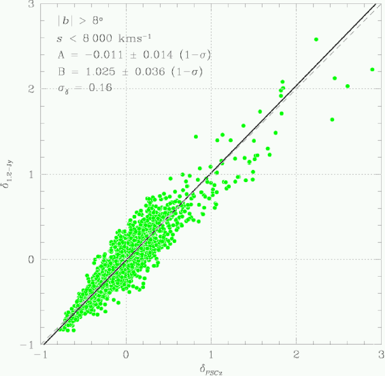
Figure 5: 1.2-Jy vs. PSCz overdensity. Only 1883 randomly selected gridpoints with $|b|>8^{\circ}$ and within $s=8\,000$ km s^-1 are shown in the scatter plot. The continuous line represents the linear best fit characterized by the zeropoint $A$ and slope $B$ indicated in the panel.

Within these limits the estimated overdensities are little affected by uncertainties in the filling-in procedure, and we expect that shot-noise dominates the total error budget. To estimate the shot-noise errors affecting both PSCz and 1.2-Jy overdensity fields we have generated 100 bootstrap realizations of the observed PSCz and 1.2-Jy surveys. These are obtained by replacing each galaxy (including the ‘synthetic’ galaxies used to fill-in the unobserved regions) with a number of objects drawn from a Poisson deviate with mean unity. Shot noise errors in $\delta$ at the generic gridpoint were set equal to the dispersion over the 100 realizations. The solid line in the plot is the best linear fit obtained from the minimization of $\chi^{2}_{\mbox{\scriptsize{eff}}}$. As shown in Tab. (2), the slope of the line, $B=1.025\pm 0.036$, is consistent with unity, indicating no systematic mismatch. On the other hand the zero-point value $A=-0.011\pm 0.014$ shows no systematic difference in the mean density of the two IRAS catalogs.

The scatter around the best–fitting line, $\sigma_{\delta}=0.16$ is similar to average shot-noise error in the 1.2-Jy density field ($\sigma_{\mbox{\scriptsize{SN}}}^{\delta_{1.2}}=0.15$). The parameter $S=\chi^{\mbox{\scriptsize{eff}}}/N_{\mbox{\scriptsize{dof}}}=0.78$ indicates that bootstrap errors slightly overestimate the true uncertainties.

4.3 Radial Density Contrast

An alternative way to characterize possible discrepancies between the two IRAS density fields is that of computing the differential radial density contrast in shells with identical thickness $\Delta s$ for both galaxy distributions:

$$\frac{\rho(s)}{\bar{\rho}}=\frac{1}{V\bar{n}}\sum_{i=1}^{N_{p}}\frac{W(s,s_{i},\Delta s)}{\phi(s_{i})},$$ (12)

where the window associated to the spherical shell $W_{\delta\rho/{\bar{\rho}}}(s,s_{i},$ $\Delta s)$ is the Heaviside function $H(s+\Delta s/2-s_{i})H(s_{i}+\Delta s/2-s)$, $s_{i}$ is the redshift of the object $i$, $V$ is the volume used to compute the mean number density ${\bar{n}}$ and the sum runs over the $N_{p}$ galaxies of the catalog. Fig. (6) shows the quantity $\rho(s)/\bar{\rho}$ for 1.2-Jy (light, dotted histogram) and PSCz (thick, continuous histogram) galaxies within $s=15\,000$ km s^-1, computed in in spherical shells of thickness $\Delta s=200$ km s^-1. Although the general shapes of two radial density contrasts are similar (with a bump at $s\sim 1\,100$ km s^-1 due to Virgo and Fornax clusters, a dip at $s\sim 3\,500$ km s^-1 induced by the Sculptor Void and a second prominent peak at $s\sim 5\,000$  km s^-1, at the same redshift as the Perseus-Pisces supercluster and the Great Attractor), a discrepancy between the two curves exists in the range $2\,000\lesssim s\lesssim 6\,000$ km s^-1 where the PSCz density is larger than the 1.2-Jy one.

The two smoothed curves in Fig. (6) show the monopole terms of the two overdensity fields $\delta_{l=0,m=0}$ as a function of radius, obtained from the spherical harmonics decomposition. Both curves interpolate the histograms rather well (hence showing the adequacy of our spherical harmonics analysis) and confirm the existence of a PSCz vs. 1.2-Jy density mismatch between the two catalogs.

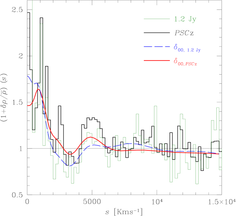
Figure 6: Differential radial density contrast for PSCz (thick line histogram) and 1.2-Jy galaxies (thin line histogram). The monopole of the PSCz and 1.2-Jy density fields are shown with smooth solid and dashed lines, respectively.

5 The IRAS PSCz and 1.2-Jy Peculiar Velocity Fields

To perform a similar analysis on the 1.2-Jy and PSCz model velocity fields we have integrated Eqn. (5) using $\beta=0.6$, a value consistent with recent determinations based on several velocity-velocity comparisons (e.g. Nusser et al. 2000), a recent density-density analysis (Zaroubi et al. 2002) and the study of mean relative velocities of galaxy pairs (Juszkiewicz et al. 2000).

5.1 Radial Peculiar Velocity Maps

To obtain maps of the radial velocity field we have computed the gradient of the velocity potential projected along the line of sight: $u({\bf s})=\hat{{\bf s}}\cdot\nabla\Phi$ at the same gridpoint positions used for the analysis of the density field.

The top end mid panels of Figs. (7-9) are similar to those of figs. 2–4 and show the radial velocity maps in the same shells. The bottom panels show the maps of the radial velocity residuals $u_{\mbox{\scriptsize{res}}}(s)\equiv u_{0.6}(s)-u_{1.2}(s)$. The thick line represents the zero radial velocity (residual) contour. The velocity (residual) contour spacing $\Delta u$ ($\Delta u_{\mbox{\scriptsize{res}}}$) varies with the redshift and is indicated in the Figure captions.

The main feature seen at all redshifts in both 1.2-Jy and PSCz radial velocity maps is the dipole pattern resulting from the LG reflex motion toward the CMB apex ($l\approx 276^{\circ},b\approx 30^{\circ}$, Kogut et al.1993).

Local deviations from this pattern arise from peculiar motions, like the infall onto Perseus-Pisces superclusters at $(s\approx 3000$  km s^-1,$~{}l\approx 120^{\circ},~{}b\approx-40^{\circ})$. The largest velocity residuals are located near the galactic plane, but their contours are broader due to the intrinsic non-locality of the peculiar velocity field. The most striking feature is perhaps the fact that velocity residuals, that are positive across a large fraction of the sky in the first shell, becomes mostly negative in the remaining two shells, suggesting possible systematic errors in either PSCz or 1.2-Jy velocity models.

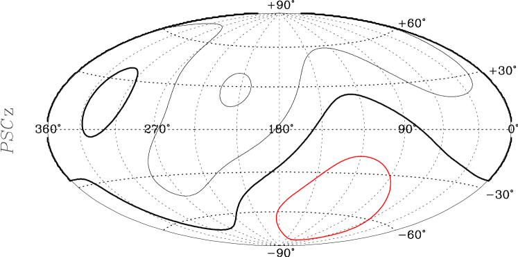
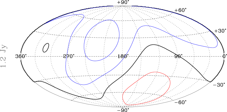
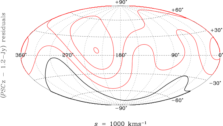
Figure 7: PSCz (top), 1.2-Jy (middle) and residual (bottom) radial velocity fields in the spherical shell centred at $s=1\,000$  km s^-1. The thick-line contour indicates $\delta u=0$ or $\Delta u_{\mbox{\scriptsize{res}}}=0$. The light- and dark-gray contours show regions characterized by outflows or infall motions. In the top and middle panels the contours are equally–spaced by $\Delta u\ =200$  km s^-1. The bottom panel shows the velocity residuals in steps of $\Delta\delta_{\mbox{\scriptsize{res}}}=25$  km s^-1.

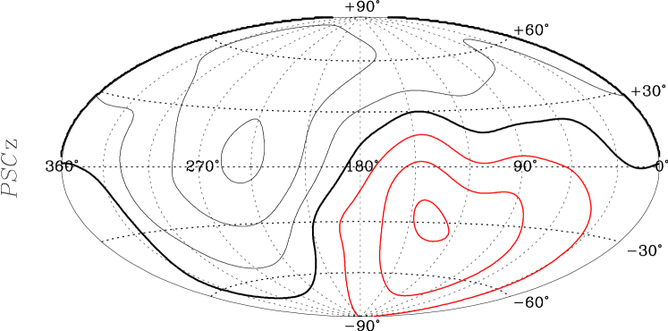
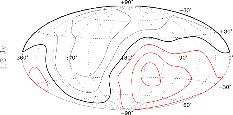
Figure 8: Same as in Fig. (7). The shell is now centred at $s=3\,000$ km s^-1and the contour spacings are $\Delta u\ =200$  km s^-1and $\Delta u_{\mbox{\scriptsize{res}}}=50$  km s^-1

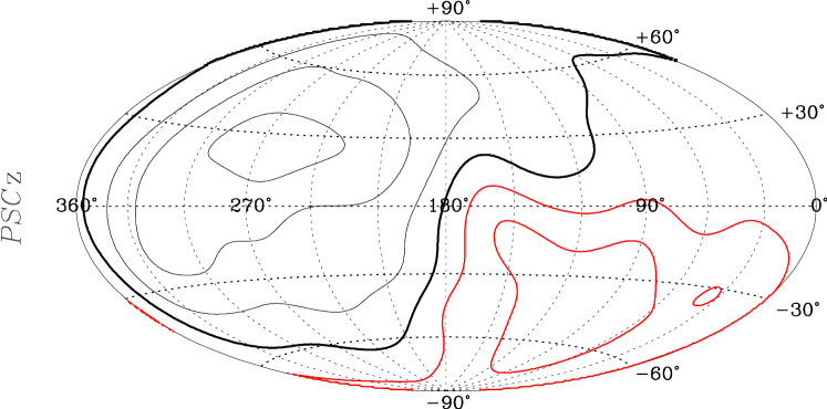
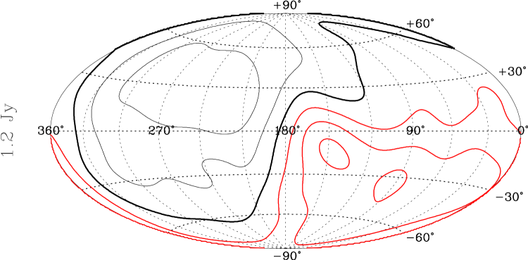
Figure 9: Same as in Fig. (7). The shell is now centred at $s=5\,000$  km s^-1and the contour spacings are $\Delta u\ =200$  km s^-1and $\Delta u_{\mbox{\scriptsize{res}}}=50$  km s^-1.

5.2 Velocity Residuals

To perform a more quantitative comparison between the two radial velocity fields we have repeated the analysis of § 4.2 and performed a linear regression between $u_{1.2}$ and $u_{0.6}$ by minimizing

$$\chi^{2}=\sum_{i=1}^{N_{\mbox{\scriptsize{grid}}}}\frac{\left(u_{1.2}-A-B\sigma_{u,0.6}\right)^{2}}{\left(u_{1.2}^{2}+B^{2}\sigma_{u,0.6}^{2}\right)},$$ (13)

where $N_{\mbox{\scriptsize{grid}}}$ runs over the same points used for the density-density comparison. Linear velocities are obtained by integrating the mass density fields over large scales causing them to be correlated on scales larger than the radius of the Gaussian kernel. This means that the number of independent gridpoint $N_{eff}$ is smaller than the estimate given by Eqn. (11). Intrinsic large scale smoothing also affects the velocity error estimate, $\sigma_{u}$ since uncertainties in modeling the galaxy distribution in the unobserved areas now add to shot noise errors.

The shot noise errors have been computed using the same bootstrap resampling technique described in § 4.2. Uncertainties in the filling-in procedure have been evaluated from 20 independent PSCz and 1.2-Jy mock catalogs extracted from the $N$-body simulations performed by Cole et al. (1997) simulating a volume of $\approx 170\,{\it h}^{-1}\,{\rm Mpc}$ in an Einstein-de Sitter universe with a non-vanishing ($\Omega_{\Lambda}=0.7$) cosmological constant and density fluctuations normalized to the observed cluster abundance (Eke, Cole & Frenk 1996 ). Model velocity fields from each IRAS mock catalog were compared with velocities obtained from ideal, all-sky IRAS mock catalogs. The variance over 20 mocks at each gridpoint quantifies the uncertainties in the filling procedure. Total uncertainties were obtained by adding in quadrature the two errors.

The results of the linear regression are summarized in Tab. (2) which shows the slope of the best fitting line $B=1.040\pm 0.019$ and the value of the zero-point, $A=60.0\pm 5.9$ km s^-1. While the slope is still consistent with unity, at the 2.1-$\sigma$ confidence level, the zero point is significantly different from zero, hence corroborating the evidence for a mismatch in the average densities of PSCz and 1.2-Jy catalogs. The dispersion around the fit is, $\sigma_{u}=88$ km s^-1  is similar to the typical velocity error computed from the IRAS mocks and the bootstrap resampling catalogs ($\sigma_{u_{0.6}}=71$ km s^-1 and $\sigma_{u_{1.2}}=140$ km s^-1). The parameter $\chi^{\mbox{\scriptsize{eff}}}/N_{\mbox{\scriptsize{dof}}}$ is less than unity which either indicates that errors are overestimated or that the value $N_{eff}$, taken from Eqn. (11), does significantly overestimate the true number of degrees of freedom.

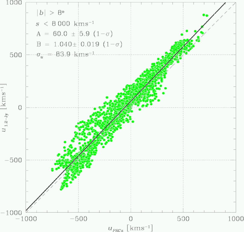
Figure 10: 1.2-Jy vs. PSCz radial velocities computed at 1883 randomly selected gridpoint positions with $|b|>8^{\circ}$ and $s\leq 8\,000$ km s^-1 inferred radial velocity field (x-axis) versus that inferred from the 1.2-Jy survey (y-axis). The parameters of the best fitting line $(A,B)$ the scatter $\sigma_{u}$ are indicated.

5.3 Velocity Multipoles

The spherical harmonics decomposition allows us to better investigate and characterize possible discrepancies between 1.2-Jy and PSCz velocity fields. Here we are only interested in the first three $(l=0,1,2)$ components, corresponding to the monopole, dipole and quadrupole terms, which have already been investigated in previous analyses (e.g. BDSLS). It is worth stressing that the monopole and dipole components at a given redshift are only sensitive to the mass distribution within the corresponding distance and thus can be directly related to the structures within the volume considered, while the quadrupole components are also sensitive to the mass distribution beyond such a distance [see Eqn. (9) in Nusser & Davis 1994].

The monopole terms of PSCz (continuous line) and 1.2-Jy (dashed line) velocity fields are plotted in Fig. (11) as a function of the redshift. The hatched and dashed regions represent the 1-$\sigma$ uncertainty strip, computed from the mock catalogs and the bootstrap resampling procedure.

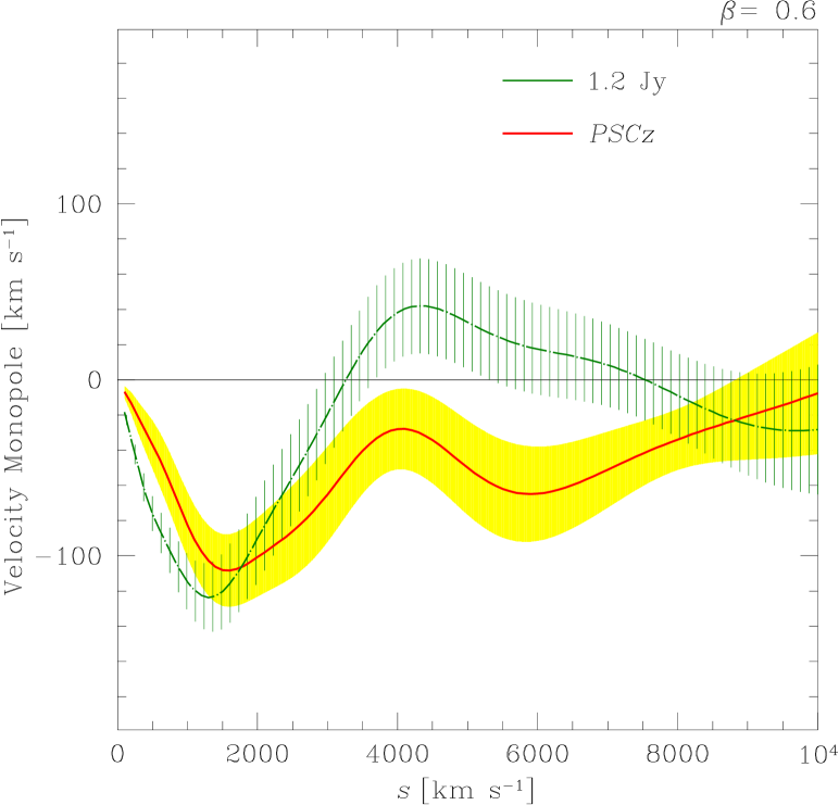
Figure 11: Monopole coefficients of 1.2-Jy (dashed) and PSCz (continuous) radial velocity fields. $1-\sigma$ errors are represented by the hatched (shaded) areas.

Both velocity monopoles display the same general features, as expected given the similarities between the density monopoles $\delta_{00}(s)$ shown in Fig. (6). There is a significant radial inflow around $s=$ 1 800 km s^-1 corresponding to the infall motion toward the Virgo-Fornax complex, an outflow in the range $1\,800\lesssim s\lesssim 4\,000$  km s^-1 due to the presence of the local void and another infall beyond this radius, due to the Hercules, Hydra, Centaurus and Perseus-Pisces superclusters. Differences between the two velocity monopoles are detected with a significance level larger than 1-$\sigma$ at very small radii ($s<1200$ km s^-1) and in the range $3500\$ km s^-1$<s<7500$ km s^-1.

Fig. (12) shows the total amplitude (lower left panel) and the three Cartesian components (remaining panels) of the two IRAS velocity dipoles. The total amplitude of the PSCz dipole (continuous line) is systematically smaller that the 1.2-Jy one (dashed line) but the discrepancy is well within the expected errors, in agreement with previous studies (e.g. Schmoldt et al. 1999).

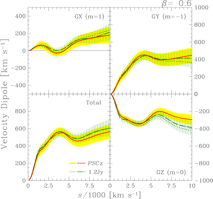
Figure 12: The velocity dipole coefficients, $u_{1m}(s)${$m=-1,0,1$}, inferred from PSCz (continuous) and 1.2-Jy (dashed) and their associated 1-$\sigma$ uncertainties. The three Galactic Cartesian components $GX$, $GY$, $GZ$ are shown in the top-left, top-right and bottom-right panel, respectively. The total amplitude is shown in the bottom-left panel. The dotted line refers to the dipole of PSCz galaxies with flux $f_{\mbox{\scriptsize{$60\mu m$}}}\geq 1.2$ Jy.

Finally, Fig. (13) shows the five components of the PSCz (continuous line) and 1.2-Jy (dashed line) velocity quadrupoles, $u_{\,2m}(s)$ (where $m=-2,...,2$) along with total amplitude (bottom-left panel). As for the dipole case, the two sets of quadrupole components agree to within 1-$\sigma$ apart from a small disagreement in the the $m=+2$ and $m=-2$ components beyond $s=7000$  km s^-1. Indeed, beyond $s\approx 6\,000$ km s^-1 the amplitude of the PSCz quadrupole decreases, while the 1.2-Jy one increases monotonically.

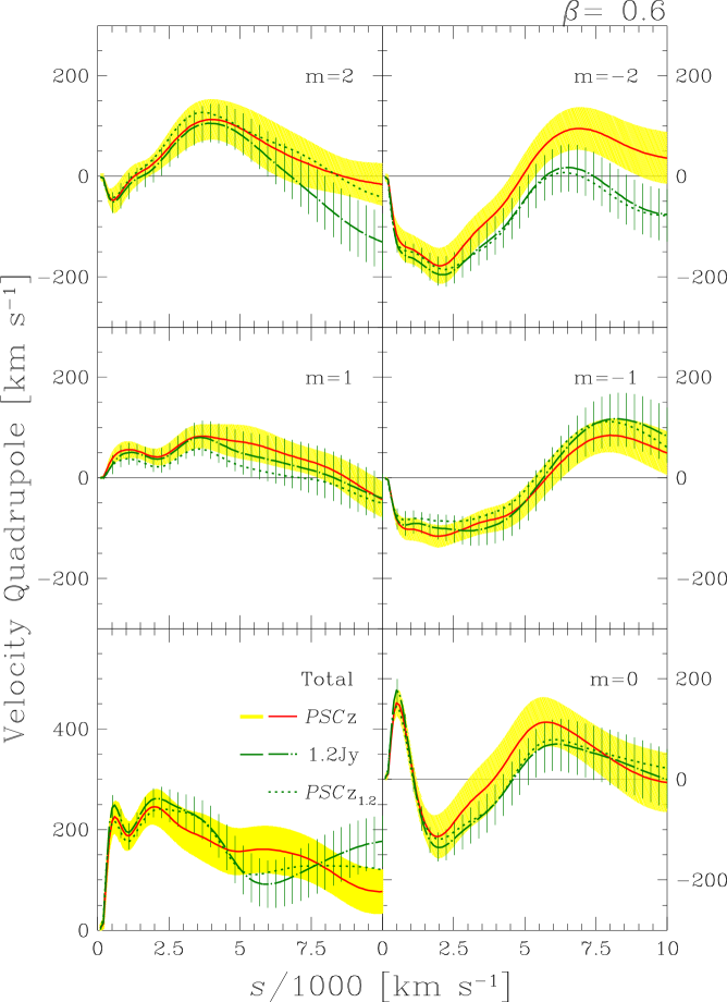
Figure 13: Quadrupole coefficients $u_{\,2m}(s)${$m=-2,...,2$} derived from PSCz (solid line) and 1.2-Jy (dashed) model velocity fields. Shaded regions indicate the $1-\sigma$  uncertainty regions. The dotted line represents the quadrupole components for PSCz galaxies with flux $f_{\mbox{\scriptsize{$60\mu m$}}}\geq 1.2$ Jy.

It is worth noticing that our 1.2-Jy velocity multipoles agree with those computed by BDSLS except that their multipole components exhibit sharper features at small radii ($s<500$  km s^-1). This mismatch derives from our use of a Gaussian smoothing kernel of radius $330$ km s^-1 which is somewhat larger than that applied by BDSLS.

6 Discussion.

Perhaps the most surprising result of our analysis is the disagreement between the PSCz and 1.2-Jy velocity monopoles in the $1\,800\lesssim s\lesssim 4\,000$  km s^-1 range. Before investigating the possible causes of this mismatch, it is worth noticing that none of our IRAS monopoles is consistent with an outward flow of magnitude $\approx 400$  km s^-1 at a distance of $7\,000$  km s^-1 like the one detected by Zehavi et al. (1998) using a sample of 44 Type Ia supernovae. That result is also at variance with the velocity model obtained from the distribution of ORS galaxies obtained by BDSLS which means that, if confirmed, it would be difficult to reconcile with the Gravitational Instability scenario.

A possible clue to understand the origin of the monopole mismatch is provided by the analysis of BDSLS that returns a velocity monopole somewhere between the PSCz and 1.2-Jy ones in the range of interest. This seems to suggest that our monopole discrepancy originates from systematic errors in one of the IRAS catalogs, possibly some incompleteness of the largest catalog at faint fluxes.

The results of Tadros et al. (1999) seem to confirm that PSCz catalog might be statistically incomplete at fluxes $f_{\mbox{\scriptsize{$60\mu m$}}}\leq 0.7$ Jy. To test whether this is indeed the case we have extracted a brighter PSCz subsample (called PSCz_0.7) by discarding all object with $f_{\mbox{\scriptsize{$60\mu m$}}}\leq 0.7$ Jy and have repeated our spherical harmonics decomposition analysis. The results, shown in Fig. (14) indicate that the PSCz_0.7 velocity monopole (dotted line) basically coincide with that of the complete sample. It is only when discarding galaxies with fluxes smaller than 1.2 Jy that the velocity monopole (dashed line) agrees with the 1.2-Jy one.

Another possibility of understanding the monopole mismatch is that of invoking a strong evolution of IRAS galaxies as a function of the redshift, which we have neglected in our calculations so far. Roughly speaking evolution can be distinguish into two different types. Pure density evolution changes only the normalization of the luminosity function while its shape is invariant with redshift. Pure luminosity evolution on the other hand describes a possible change of the intrinsic luminosities of the sources but not their number density. Both forms of evolution occur simultaneously in the Universe. For instance, galaxy merging reduces the number density of galaxies causing thus evolution. Besides, such events also cause different luminosities of the final systems and hence leading to luminosity evolution. Other physical mechanism for galaxy evolution can be devised. Some evidences for a sizable evolution of IRAS galaxies have been reported by a number of authors, although there seem to be much controversy about the amplitude of the effect (see Springel 1996 and references therein).

Canavezes et al. (1998) expressed evolution in terms of a generalization of the selection function introduced by Yahil et al. (1991) given by

$$\phi(s)_{\mbox{\scriptsize{evol}}}=\left\{\begin{array}[]{ll}\left(\frac{r_{s}}{r}\right)^{\alpha}\left(\frac{r_{\star}^{\gamma}+r_{s}^{\gamma}}{r_{\star}^{\gamma}+r^{\gamma}}\right)^{\beta/\gamma}&\quad,~{}s\geq H_{0}r_{s},\\ 1&\quad,~{}\mbox{otherwise.}\\ \end{array}\right.$$ (14)

Springel (1996) showed that it indeed provides a rather accurate modeling of both IRAS data-sets. The estimated parameters using a maximum-likelihood procedure are listed in Tab. (1) and are denoted by PSCz${}_{\mbox{\scriptsize{evol}}}$. The effect of evolution are shown in Fig. (14) in which the velocity monopole term derived from the PSCz galaxy distribution in which evolutionary effects have been accounted for through the new selection function $\phi(s)_{\mbox{\scriptsize{evol}}}$ (dot–dashed line) is plotted against the unevolved model. The evolutionary effects are very minor, as was somewhat expected given the locality of our galaxy sample, and do not help in reducing the PSCz vs. 1.2-Jy velocity monopole mismatch.

Overall, our analysis seems to indicate that the discrepancy between 1.2-Jy and PSCz velocity monopoles cannot be ascribed to errors in the modeling of the selection function which, as we have seen, would not change the monopole terms appreciably. Catalog incompleteness at very low fluxes has to be ruled out too. We can only conclude that either the PSC$z$ incompleteness extend at objects with fluxes comparable to 1.2 Jy or that the monopole mismatch does reflect a genuine difference in the average density of faint vs. bright IRAS galaxies at $s\leq 4000$  km s^-1.

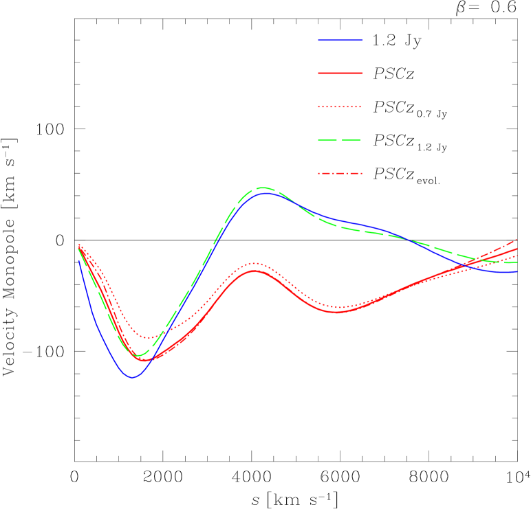
Figure 14: Velocity monopoles for the 1.2-Jy (dark gray line) PSCz (light-gray), PSCz_0.7 (dot-dashed), PSCz_1.2 (long-dashed) PSCz${}_{\mbox{\scriptsize{evol}}}$ (dotted) samples.

Table 3: Selection function parameters In the IRAS mock catalogs.

Mock catalog	$\alpha$	$\beta$	$r_{s}$	$r_{\star}$
			$[\,{\it h}^{-1}\,{\rm Mpc}]$	$[\,{\it h}^{-1}\,{\rm Mpc}]$
PSCz	0.53	1.90	10.90	86.40
1.2-Jy	0.48	1.79	5.00	50.40

A second important result found in our analysis is that the 1.2-Jy and PSCz dipoles agree within the 1-$\sigma$ errors. This means that the use of the PSCz rather than the 1.2-Jy catalog does not help in reducing the Mark III-IRAS dipole residuals found by Davis, Nusser & Willick (1996). Indeed, both GX and GY components of the PSCz velocity dipole are much too large with respect to Mark III ones (see Fig 15 of Davis, Nusser & Willick 1996). Similar results were also obtained from the ORS vs. Mark III dipole velocity comparison (BDSLS). We conclude that the discrepancy between the Mark III and 1.2-Jy velocity fields cannot be alleviated by reducing the shot noise errors of the model velocity field.

The agreement between the PSCz, 1.2-Jy and ORS dipoles is reassuring since it guarantees that uncertainties in model velocity fields arising from within the galaxy samples that derive from incompleteness in one (or more) catalogs, incorrect treatment of non-linear velocities or non-linear non-uniform biasing do not generate systematic errors apart from a the monopole mismatch in the range $1\,800$ km s^-1$\leq s\leq 4\,000$  km s^-1.

Unlike the case of monopole and dipole moments, possible differences between the 1.2-Jy and PSCz quadrupole components can also be attributed to incorrect determination and dilute sampling of the density field beyond the sample. The fact that 1.2-Jy and PSCz velocity quadrupole agree within the expected errors suggests that differences in the quadrupole components of the two fields can be understood in terms of shot noise errors and uncertainties in filling the empty regions.

With this respect it is worth investigating whether the denser sampling of the PSCz catalog at large radii allows a better modeling of the large scale contribution to the model velocity field. Indeed, when comparing the model 1.2-Jy velocity field to Mark III velocities in the framework of the VELMOD analysis, WSDK have found that velocity residuals exhibit a quadrupole pattern of the form $u_{\mathcal{Q}}=\mathcal{V}_{\mathcal{Q}}\,{\bf r}\,\cdot\,\hat{{\bf r}}$, where $\mathcal{V}_{\mathcal{Q}}$ is a traceless, symmetric $3\times 3$ tensor. They have attributed this “VELMOD quadrupole” residuals to uncertainties in modeling the IRAS density field beyond $3\,000$  km s^-1. In particular they found that the most important sources of uncertainties were the smoothing procedure (based on a Wiener Filtering technique) and the shot noise errors, with the errors deriving from having ignored mass inhomogeneities beyond $12,000$  km s^-1 playing a minor role. Using PSCz instead of 1.2-Jy catalog reduces the shot noise errors in the density field beyond $3000$  km s^-1 and thus should improve the agreement with the Mark III velocities. In other words one would expect the quadrupole of the residual velocity field $u^{>}_{0.6}-u^{>}_{1.2}$, where one only takes in account the mass beyond $3000$  km s^-1, to be similar to the “VELMOD quadrupole” of WSDK.

In Fig. (15) we compare the VELMOD quadrupole at $s=2000$ km s^-1 (rescaled from $\beta=0.492$ to $\beta=0.6$, upper panel) to the $u^{>}_{0.6}-u^{>}_{1.2}$ quadrupole residual (lower panel). The VELMOD quadrupole reaches its maximum value at $(l\approx 165^{\circ},~{}b\approx 55^{\circ})$ and in the opposite direction of the sky. The $u^{>}_{0.6}-u^{>}_{1.2}$ residual quadrupole exhibits a rather different pattern, reaching its maximum amplitude at $(l\approx 156^{\circ},~{}b\approx-74^{\circ})$. The value of the quadrupole components of 1.2-Jy and PSCz as well as those of the VELMOD and $u^{>}_{0.6}-u^{>}_{1.2}$ quadrupole residuals computed at a distance of 2000  km s^-1  are shown in Tab. (4). This comparison is at best qualitative since (i) VELMOD quadrupole is computed in real space while both IRAS quadrupoles refer to redshift space insted, and (ii) the smoothing scheme used in WDKS is different from with ours.

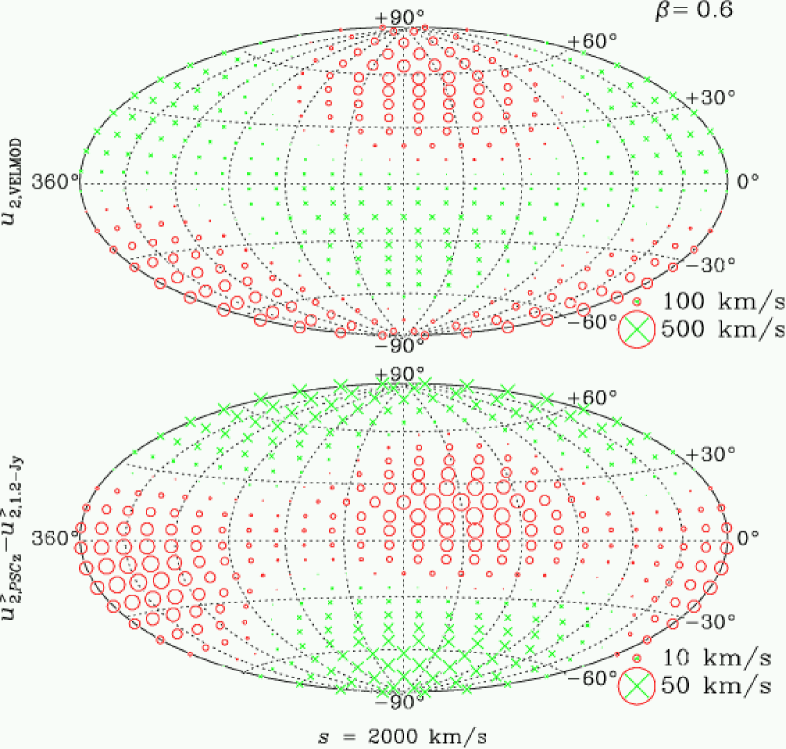
Figure 15: VELMOD (upper panel) and $u^{>}_{0.6}-u^{>}_{1.2}$ (lower panel) quadrupole residuals at $s=2\,000$ km s^-1. Stars denote outflowing from us (LG frame); circles denote infall to us. The size of the symbol is proportional to the amplitude of the flow (notice the different velocity scales in the two panels). The maximum amplitude of the “VELMOD quadrupole” (top panel) is $\approx$ 181 km s^-1, while for $u^{>}_{0.6}-u^{>}_{1.2}$ is $\approx$ 23  km s^-1.

Table 4: Quadrupole Components at $2\,000$ km s^-1

	VELMOD	PSCz	1.2-Jy	PSCz  - 1.2-Jy
	[ km s-1]	[ km s-1]	[ km s-1]	[ km s-1]
$\cal{V}_{Q}$ (x,x)…	45	57	69	-13
$\cal{V}_{Q}$ (y,y)…	44	-22	-15	-7
$\cal{V}_{Q}$ (z,z)…	-89	-35	-54	20
$\cal{V}_{Q}$ (x,y)…	18	-150	-156	6
$\cal{V}_{Q}$ (x,z)…	138	57	48	10
$\cal{V}_{Q}$ (y,z)…	-29	-106	-102	-5

NOTE.–(1) We have rescaled the “VELMOD quadrupole” components presented in WSDK’s Tab. (2) to the numerical value of $\beta=0.6$.

7 Conclusions.

We have compared the model velocity and density fields of the PSCz survey to those derived from the sparser 1.2-Jy sample in redshift space. Our model predictions are based on the Nusser & Davis (1994) spherical harmonics decomposition technique and assumes Zeld’ovich approximation and linear biasing.

The IRAS overdensity fields are reconstructed with a smoothing proportional to the 1.2-Jy inter-galaxy separation and exhibit the same general features corresponding to the known cosmic structures in the local universe. The model velocity field, computed in the LG frame, has a dipole–like appearance, with galaxies moving away from us toward Perseus-Pisces region and approaching the LG from the opposite direction.

The analysis of the velocity multipoles has revealed a significant discrepancy between the PSCz and 1.2-Jy velocity mono- poles in the range $1\,800\lesssim s\lesssim 4\,000$ km s^-1 in which PSCz radial velocities are systematically larger than 1.2-Jy ones, that cannot be explained by uncertainties in the IRAS selection functions or incompleteness of the PSCz catalog at faint fluxes. Also, the mismatch cannot be ascribed to errors derived from shot–noise and treatment of unobserved areas since both have been accounted for with the help of realistic mock IRAS catalogs and the extensive application of bootstrap resampling techniques to both IRAS datasets.

Both IRAS dipole and quadrupole moments are in good agreement within the sampled volume apart from a small mismatch in the $u_{10}$, $u_{2,-2}$ and $u_{22}$ quadrupole components beyond $s=7\,000$ km s^-1. The agreement between the dipole moments and their consistency with the velocity dipole computed by BDSLS from the ORS catalog suggests that deviations from homogeneous linear biasing prescriptions have to be small and cannot be advocated to explain the aforementioned mismatch between the IRAS monopoles.

Another remarkable consequence of the agreement among the various dipoles is that the 1.2-Jy-Mark III residuals cannot be alleviated by using the PSCz catalog instead of the 1.2-Jy or the ORS ones. In fact, this suggests that the origin of the 1.2-Jy-Mark III dipole resides in the Mark III calibration procedure; a suggestion corroborated by the fact that the dipole mismatch disappears when adopting the alternative VELMOD procedure to calibrate -Mark III velocities (WDSK). The VELMOD analysis requires a sizable external quadrupole component within $3000$  km s^-1. This quadrupole accounts for uncertainties errors in the 1.2-Jy model density field beyond that distance. We found that using the PSCz sample provides part of the required external tidal field.

As a final remark, we would like to stress that the present analysis illustrates once more the importance of spherical harmonics decomposition techniques to compare observed and model density and velocity fields obtained from all-sky samples, to reveal possible data-model or model-model inconsistencies and to assess model adequacy. These techniques will prove very useful when the next generation of all-sky redshift surveys and peculiar velocity catalogs [e.g. the 6dF (http:www.mso.anu.edu.au/6dFGS) and 2MRS (http:cfa-www.harvard.edu/huchra/2mass) datasets] will become available.

Ackowledgements

We thank Adi Nusser for enlightening discussions. LT was partly funded by FCT (Portugal) under the grants PRAXIS XXI /BPD/16354/98, PRAXIS/C/FIS/13196/98 and POCTI/1999/ FIS/36285. LT aknowledges the hospitality of the Aspen Center for Physics and the Kvali Institute for Theoretical Physics where much of the work was completed.

References

- Baker et al (1999) Baker, J. and Davis, M. and Strauss, M. A. and Lahav, O. and Santiago, B., 1999, ApJ, 508, 6
- Branchini et al (1999) Branchini, E. and Teodoro, L. and Frenk, C. S. and Schmoldt, I. and Efstathiou, G. and White, S. D. M. and Saunders, W. and Sutherland, W. and Rowan-Robinson, M. and Keeble, O. and Tadros, H. and Maddox, S. and Oliver, S., 1999, MNRAS,308, 1
- Bunn (1995) Bunn, E. F., 1995, PhD thesis, University of California, Berkeley
- Canavezes et al (1998) Canavezes, A. and Springel, V. and Oliver, S. J. and Rowan-Robinson, M. and Keeble, O. and White, S. D. M. and Saunders, W. and Efstathiou, G. and Frenk, C. S. and McMahon, R. G. and Maddox, S. and Sutherland, W. and Tadros, H., 1998, MNRAS, 297, 777
- Cole etal (1997) Cole, S., Weinberg, D. H., Frenk, C. S., and Ratra, B.,1997, MNRAS, 289, 37
- Colless et al (2001) Colless, M. and Dalton, G. and Maddox, S. and Sutherland, W. and zes Norberg, P. and Cole, S. and Bland-Hawthorn, J. and Bridges, T. and Cannon, R. and Collins, C. and Couch, W. and Cross, N. and Deeley, K. and De Propris, R. and Driver, S. P. and Efstathiou, G. and Ellis, R. S. and Frenk, C. S. and Glazebrook, K. and Jackson, C. and Lahav, O. and Lewis, I. and Lumsden, S. and Madgwick, D. and Peacock, J. A. and Peterson, B. A. and Price, I. and Seaborne, M. and Taylor, K., 2001, MNRAS, 328, 1039
- daCosta et al (2000) da Costa, L. N. and Bernardi, M. and Alonso, M. V. and Wegner, G. and Willmer, C. N. A. and Pellegrini, P. S. and Rité, C. and Maia, M. A. G., 2000, ApJ, 120, 95
- Davis et al (1996) Davis, M. and Nusser, A and Willick, J., 1996, ApJ, 473, 22
- Dekel et al (1993) Dekel, A. and Bertschinger, E. and Yahil, A. and Strauss, M. A. and Davis, M. and Huchra, J. P., 1993, ApJ, 412, 1
- Dekel et al (1999) Dekel, A. and Eldar, A. and Kolatt, T. and Yahil, A. and Willick, J. A. and Faber, S. M. and Courteau, S. and Burstein, D., 1999, ApJ, 522, 1
- Eke et al (1996) Eke, V., Cole, S., and Frenk, C.: 1996, MNRAS, 282, 263
- Fisher et al (1995a) Fisher, K. B. and Huchra, J. P. and Strauss, M. A. and Davis, M. and Yahil, A. and Schlegel, D., 1995, ApJS, 100, 69
- Fisher et al (1995b) Fisher, K. B. and Lahav, O. and Hoffman, Y. and Lynden-Bel, D. and Zaroubi, S., 1995, MNRAS, 272, 219
- Haynes et al (1999) Haynes, M. P. and Giovanelli, R. and Salzer, J. J. and Wegner, G. and Freudling, W. and da Costa, L. N. and Herter, T. and Vogt, N. P., 1999, ApJ, 117, 1668
- Hernquist:et al (1989) Hernquist, L. and Katz, N., 1989, ApJS, 70, 419
- Kogut et al (1993) Kogut, A., Linewater, C., Smoot, G., Bandey, C. B. A., N.W.Boggess, Cheng, E., Amici, G. D., Fixsen, D., Hinshaw, G., Jackson, P., Janssen, M., Keegstra, P., Loewenstein, K., Lubin, P., Mahter, J., Tenorio, L., Weiss, R., Wilkinson, D., and Wright, E., 1993, ApJ, 419, 1
- Lahav et al (1994) Lahav, O. and Fisher, K. B. and Hoffman, Y. and Scharf, C. A. and Zaroubi, S.,
- Jackson (1999) Jackson, J., 1999, Classical Electrodynamics, New York: Wiley
- Juszkiewicz et al (2000) Juszkiewicz, R. and Ferreira, P. G. and Feldman, H. A. and Jaffe, A. H. and Davis, M., 2000, Science, 287, 109
- Nusser & Davis (1994) Nusser, A. and Davis, M. , 1994, ApJ, 421, L1
- Nusser et al (2000) Nusser, A. and da Costa, L. N. and Branchini, E. and Bernardi, M. and Alonso, M. V. and Wegner, G. and Willmer, C. N. A. and Pellegrini, P. S., 2000, MNRAS, 320, L21
- Rowen-Robinson et al (1990) Rowan-Robinson, M. and Lawrence, A. and Saunders, W. and Crawford, J. and Ellis, R. and Frenk, C. S. and Parry, I. and Xiaoyang, X. and Allington-Smith, J. and Efstathiou, G. and Kaiser, N., 1990, MNRAS, 247, 1
- Saunders et al (2000) Saunders, W. and Sutherland, W. J. and Maddox, S. J. and Keeble, O. and Oliver, S. J. and Rowan-Robinson, M. and McMahon, R. G. and Efstathiou, G. P. and Tadros, H. and White, S. D. M. and Frenk, C. S. and Carramiñana, A. and Hawkins, M. R. S., 2000, MNRAS, 317, 55
- Sigad et al (1998) Sigad, Y. and Eldar, A. and Dekel, A. and Strauss, M. A. and Yahil, A., 1998, ApJ, 495, 516
- Springel (1996) Springel, V.,1996, MSc thesis, Eberhard-Karls-Univerität Tübingen
- Strauss & Willick (1995a) Strauss, M. A.and Willick, J. A., 1995, PhR, 261, 271
- Zaroubi et al (2002) Zaroubi, S. and Branchini, E. and Hoffman, Y. and da Costa, L. N., 2002, MNRAS, 336, 1234
- Tadros et al. (1999) Tadros, H., Ballinger, W. E., Taylor, A. N., Heavens, A. F., Efstathiou, G., Saunders, W., Frenk, C. S., Keeble, O., MCMahon, R., Maddox, S. J., Oliver, S., Rowan-Robinson, M., Sutherland, W. J., and White, S. D. M.: 1999, MNRAS, 305, 527
- Teodoro (1999) Teodoro, L., 1999, PhD thesis, University of Durham
- Willick et al (1997) Willick, J. and Strauss, M. and Dekel, A. and Kolatt, T., 1997, ApJ, 486,629
- Willick et al (1997a) Willick, J. and Courteau, S. and Faber, S. and Burstein, D. and Dekel, A. and Strauss, M. A., 1997, ApJS, 109, 333
- Willick & Strauss (1998) Willick, J. and Strauss, M. A., 1998, ApJ, 507, 64
- (33) Yahil, A. and Strauss, M. A. and Davis, M. and Huchra, J., 1991, ApJ, 372, 380
- York et al (2000) York, D. G. et al., 2000, ApJ, 120, 1579
- Zehavi et al (1998) Zehavi, I. and Riess, A. G. and Kirshner, R. P. and Dekel, A., 1998, ApJ, 503, 483